HAL Id: hal-02318327
https://hal.archives-ouvertes.fr/hal-02318327
Submitted on 16 Oct 2019
HAL is a multi-disciplinary open access
archive for the deposit and dissemination of
sci-entific research documents, whether they are
pub-lished or not. The documents may come from
teaching and research institutions in France or
abroad, or from public or private research centers.
L’archive ouverte pluridisciplinaire HAL, est
destinée au dépôt et à la diffusion de documents
scientifiques de niveau recherche, publiés ou non,
émanant des établissements d’enseignement et de
recherche français ou étrangers, des laboratoires
publics ou privés.
Classifier Training from a Generative Model
Thanh Dat Pham, Anuvabh Dutt, Denis Pellerin, Georges Quénot
To cite this version:
Thanh Dat Pham, Anuvabh Dutt, Denis Pellerin, Georges Quénot. Classifier Training from a
Gen-erative Model. CBMI 2019 - 17th International Conference on Content-Based Multimedia Indexing,
Sep 2019, Dublin, Ireland. �hal-02318327�
Classifier Training from a Generative Model
Pham Thanh Dat
Univ. Grenoble Alpes, CNRS, Grenoble INP, LIG,F-38000 Grenoble France thanh-dat.pham@ etu.univ-grenoble-alpes.fr
Anuvabh Dutt
Univ. Grenoble Alpes, CNRS, Grenoble INP, LIG,F-38000 Grenoble France anuvabh.dutt@ univ-grenoble-alpes.fr
Denis Pellerin
Univ. Grenoble Alpes,CNRS, GIPSA-Lab, F-38000 Grenoble, France [email protected]
Georges Quénot
Univ. Grenoble Alpes, CNRS, Grenoble INP, LIG,F-38000 Grenoble France [email protected]
Abstract—We investigate the samples derived from generative adversarial networks (GAN) from a classification perspective. We train a classifier on generated samples and on real data and see how they compared on a held out validation set. We see that recent GAN models which produce visually convincing samples are not yet able to match the training on real data. To analyse this we compare training a classifier on generated samples and various sizes of the real training set. We propose architectural and algorithmic changes to reduce this gap. First, we show that a modification to the GAN architecture is needed, which leads to improve generation of samples. Second, we use multiple GAN models as a way to cover the real data distribution, again leading to improvement in classifier training. We also show that in the case of training on small number of samples, a GAN model provides better compression in terms of storage requirements as compared to the real data.
Index Terms—Generative models, Generative adversarial net-works, deep learning.
I. INTRODUCTION
Deep convolutional networks have had success in various image tasks such as image classification, object detection and segmentation. In all these tasks, these models have performed the best as measured by various criteria. On the other side, generative models such as Generative Adversarial Networks [1] and Variational Autoencoders (VAE) have been proposed and demonstrated to generate images with reasonable similarity to the real training data. Recent advances especially in GANs, such as BigGAN [2] have produced samples which are quite hard to distinguish from real data. In this work, our primary objective is to be able to train good discriminative classifiers from the samples of a generative model. The ability to do this has several applications such as data compression and data privacy protection. A generative model can be thought of as a compressed version of the real data. In a scenario where it is not possible to store or share the real data, we can instead have the compressed generative model. In several applications, such as in the medical domain, data sharing may not be possible due to factors such as protecting data of patients. In these case we can instead share the generative model, and others can reuse this data for other applications, without compromising privacy. In this work, our aim is to see how the current state-of-the-art GAN model samples compare with real data samples, when compared from the perspective of training a classifier on these samples. In order to compare generated samples to real data
several metrics have been proposed such as Inception Score (IS) [3] and Fréchet Inception Distance (FID) [4]. These metrics aim to characterise how real-like the generated samples. In this work we are interested in training a discriminative classifier model from the samples of a trained generative model. Indeed we also investigate if good IS and FID scores correlate with training of good classifiers.
First we train a classifier from the samples of BigGAN [2] and compare the training with real data samples. This is to evaluate the extent of correlation between visually convincing samples and the ability to train good classification models. We present a generative model as a compressed view of real data and show that in low data regimes a generative model can be efficient to store the data as compared to the raw data itself. Next, we propose a modification of the building block of the generator and discriminator, which leads to generation of samples that give better classifiers as measured by validation error. We find that in the residual blocks using a concatenation operation instead of addition leads to increased quality and diversity of generated samples. Finally, we show that using combining samples from multiple generative models leads to a better coverage of the real data distribution.
II. RELATEDWORK
Background. Generative Adversarial Networks (GAN) [1] is a type of generative model whose training procedure involves a two player game between a generator network which produces samples, and a discriminator network which classifies samples as either coming from the generator or real data. The discriminator network serves as the loss function for training the generator network. There has been several improvements to the original GAN model involving architectural and optimisation advancements. The recently proposed BigGAN [2] model presents a framework for training GANs and produces very visually rich samples that are quite hard to distinguish from real data.
Conditional-GAN [5] presents the framework for sampling from a GAN based on a conditioning factor, such as image category. Most early work on GAN had focused on uncon-ditional training of GAN. There is not clear evidence as to where in the network the conditioning information is to be provided and different techniques have been proposed, such as providing a one-hot class embedding at the input,
or a learnt class embedding in one of the internal layers. Conditional batch normalisation [6] layers have been found to be effective for modulating the activations in a network and have been subsequently used for conditional image generation in GANs [2], [7].
View of GANs from a classification perspective. Training and evaluating classifiers on GAN samples have been investi-gated in [8], where the authors have compared the classification error with other evaluation metrics such as Inception Score (IS) and Fréchet Inception Distance (FID). In this work our aim is not to compare different metrics and improve them but to solely improve the validation error of a classifier on real test samples, after training a classifier on generated data only. Samples from a GAN have been investigated before from the perspective of classification in [9]. This work focuses on a similar study with recent state-of-the-art GAN models. In contrast to [9] who train a separate GAN model per category, we train class conditional GANs. This should result in better GAN models since the learning procedure has access to more data and may also help the model to learn to generate more diverse samples by making use of inter class information. We aim to see how the BigGAN model which produces visually meaningful samples compares to other GAN models in terms of classification performance when a classifier is trained on samples generated from its synthetic samples. We ask the question if visually convincing samples correspond to enabling good training of classifiers. We propose methods to obtain an improvement in training classifier from generated samples only.
III. METHOD
A. Sample filtering
Image samples obtained from a conditional GAN may not correspond to the correct category or may not be of a good enough quality. This is due to the fact that we are not able to train perfect generative models. We propose to use a pre-trained classifier, trained on the same training data as the GAN, to filter out such samples. This is a general approach that can scale to larger datasets and categories. The procedure for selecting a sample image from the GAN that will be used to train a classifier is described in Algorithm 1.
Algorithm 1: Selecting samples from the generator input : C, G, θG, Classpre, thresh
output : List of samples sample_list = []; y ∼ U (0, C); z ∼ N (0, 1); x ∼ G(z, y; θG);
p = Classpre(x);
if argmax(p) == y and p[y] > thresh then add x to sample_list
end
We can choose different threshold values for the prediction probability obtained from the pre-trained classifier. This ensures that we get samples that belong to the correct category and are also informative enough to train good classifiers. We discuss the results of training a classifier and the effect of choosing different probability thresholds in §IV-B.
B. Concatenation residual block for generator and discrimina-tor
Residual blocks have been very successful in image classi-fication tasks [10]. The operation of a residual block can be defined as y = F (x) + x, where y is the output, x is the input and F is a learned transformation of x, usually a series of convolution, batch norm and ReLU activation layers. Residual blocks have been used as the building block of generator and discriminator networks in recent GAN models [2], [7].
In the classifier setting, DenseNet [11] has proposed using concatenation instead of addition in the residual blocks and this has been shown to perform better in discriminative image tasks. This can be written as: y = Conv1×1(concat(F (x), x)).
The 1 × 1 convolution operation is used to reduce the number of channels and keep them the same as in the case of residual blocks. This modification leads to improvement in the quality of generated samples and is discussed in §IV-D.
C. Multiple GAN sampling
Our training datasets are that of natural images which have significant variation among categories and also within each category. We expect that this implicit distribution is difficult for current generative models to capture. Current hypothesis suggests that generative models suffer from mode collapse which leads to the model being unable to capture all aspects of the data distribution. We can train multiple GAN models on the same dataset to cover more of this distribution, where each GAN model might be able to model different parts of the distribution. We hypothesise that this might be possible due to different starting initialisation and non-convex loss surface during the training procedure of the GAN model. During training of the classifier from synthetic samples, we can construct our dataset by sampling from these multiple GAN models which can help us to cover the data distribution in a more effective manner. Experiments and results are discussed in §IV-E.
IV. EXPERIMENTS
A. Datasets and models
We experiment on the CIFAR-10 and CIFAR-100 [12] datasets. These datasets consist of 50 000 training images divided into 10 and 100 categories respectively. Each image is 32x32 pixels and 3 channel RGB. We choose this dataset because GAN training needs large time and computational resources. CIFAR-100 provides sufficiently complex images while still being possible to train in a reasonable time. We refer to the original dataset as DR. We construct a synthetic
dataset by sampling images from a trained GAN model and
refer to it as DG. Sample images from each class are shown
in Figure3.
We use the BigGAN [2] architecture as our GAN model and it is trained according to the original paper with related settings of the hyper-parameters. For the classifier we use a 18 layer ResNet [10] model with 11M parameters because it provides a good trade off between performance and training time.
B. Classifier performance comparison between real and gen-erated data
The classifier is trained on both DR and DG is done for
156 250 steps. In the case of DR this means iterating over the
same samples multiple times as is done usually. In the case of DG a batch of samples is obtained from the trained GAN
model. We expect in the ideal case to have different image samples,however in reality we are limited by the capacity of the GAN model with respect to diversity of the data.
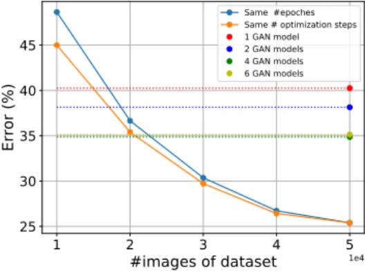
We can view a trained GAN as a compressed version of our training data, where the learned weights are the compressed representation of our original data bits. We are interested in compressing the nature of the distribution from which the training data has been sampled, rather than the explicit training data samples themselves. To measure the degree of compression we train a classifier on samples from a GAN and measure the prediction error on a held out validation set. The lower bound for the error that the classifier can achieve is equal to the error that it achieves after training on real training data. We compare training on the GAN samples with varying amounts of real training data (see Figure1and Figure2, detailed results are in TableI).
The blue curve depicts training on different subset sizes for 200 epochs. This means that in case of smaller dataset sizes, we have less number of optimisation steps. The orange curve shows training on each subset for the same number of optimisation steps. We see that in the case of less samples, training longer reduces the classification error rate substantially. The same classifier is trained on GAN samples, for the same number of optimisation steps and following the same learning rate decay schedule. Each batch of samples for training the classifier are generated according to Algorithm 1. The error rate for these classifiers is comparable to training on 1 × 10⁴ and 1.5 × 10⁴ real data samples in CIFAR-10 and CIFAR-100 respectively. This indicates that the GAN is either not able to produce samples similar to the real data or the intra class diversity is not as much as in the real dataset. The size of the GAN model is around 15MB as compared to the 30MB for the 10 × 103 samples. This shows that with a GAN we are able to obtain good compression.
C. Effect of selection threshold
A GAN sample is used for training the classifier if it belongs to the correct category and if the output probability is above a pre-defined threshold. In Figure 5we plot the relationship between output probability of the pre-trained classifier and the final validation accuracy of the classifier trained on GAN
1 2 3 4 5
#images of dataset
1e46 8 10 12 14
Error (%)
Same #epoches Same # optimization steps 1 GAN model 2 GAN models 4 GAN models 6 GAN modelsFig. 1. Training a classifier on real data compared with training on GAN samples in CIFAR-10.
1 2 3 4 5
#images of dataset
1e425 30 35 40 45
Error (%)
Same #epoches Same # optimization steps 1 GAN model 2 GAN models 4 GAN models 6 GAN modelsFig. 2. Training a classifier on real data compared with training on GAN samples in CIFAR-100.
samples. We observe that the value of the threshold is not significant in the case of CIFAR-10. This implies that the pre-trained classifier is quite confident if makes a correct prediction. The reason for this could be that the GAN is able to generate very good images and the classifier is therefore confident in its predictions. In our experiments this implies that if the pre-trained classifier makes a correct prediction in most cases we can use the corresponding sample in our synthetic training set. We need to study this further for different data sets with varying number of target classes.
However, in the case of CIFAR-100, the probability threshold is important and increasing the threshold leads to a reduction of the classifier error from 39.35% to 37.62%. The threshold makes sure that only good quality image are used for training the classifier. On the other hand, a high value of threshold can reduce the diversity of generated samples which might lead to worse generalisation for the classifier.
1) Filtering threshold analysis: At this filtering stage we can analyse which categories are filtered out more. This would be one indication that the GAN model has trouble to capture the distribution for these categories. We can further analyse the predictions and features of the pre-trained classifier for the generated samples. Similar predictions and features would indicate the repetition of samples and lack of diversity. This can be done both at the inter and intra class level. More details
Fig. 3. Several samples before filtering out bad images with dataset CIFAR-10.
Fig. 4. Several samples after filtering out bad images with dataset CIFAR-10.
will be explained in next section.
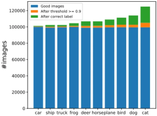
We can see in Figure6, most bad images already are removed because of incorrect label in CIFAR-10. This is one reason why the threshold value does not have too much effect. On the other hand, in Figure 7we see that in the case of CIFAR-100, the number of bad images which is filtered out by threshold value increase remarkably. There are a few categories for which it is easy to generate images belonging to the correct category, while for the majority of categories we need to sample repeatedly to get images of the correct category (green bar in Figure7). One concern here can be that for these hard categories, the intra category diversity is reduced when we sample repeatedly since the generator model is inherently of limited capacity. This can be a subject of future work, to investigate and improve diversity for hard categories. We visualise several samples before and after filtering out the bad one in Figure 3 and Figure4.
In both datasets we see that the use of the pre-trained classifier is useful for removing samples that do not belong to the correct category. The effect of the probability threshold selection becomes more important as the number of categories increases. It has a significant effect in improving the validation error of the classifier trained on generated samples.
D. Concatenation residual block for BigGAN model with CIFAR-100
In the case of CIFAR-100, for training a GAN we introduce concatresidual blocks for the generator and discriminator, as
0.4 0.6 0.8
Threshold
37.75 38.00 38.25 38.50 38.75 39.00 39.25Error (%)
11.5 11.6 11.7 11.8 11.9 12.0Error (%)
CIFAR100 CIFAR10Fig. 5. Effect of threshold on classifier training from GAN samples in CIFAR-100.
car ship truck frog deer horseplane bird dog cat 0 20000 40000 60000 80000 100000 120000
#images
Good images After threshold >= 0.9 After correct labelFig. 6. Distribution of samples belong to the classes in CIFAR-10.
explained in §III-B. This architectural change leads to signifi-cant reduction in error for classifier training, and improvements in IS and FID scores for the generator. Details are given in CIFAR-100 Concat section of TableI. concat block improves the classification error from 40.25%, for the original block, to 37.78%, and FID score from to 8.68 from 9.19. This is comparable to a model which is trained with 20 × 103real data
samples. The models uses 37.6 MB for storage as compared to 60MB for 20 × 103data samples. Using 4 GAN models, the test error is further reduced by 3%. Figure8and Figure9show
0 20 40 60 80 100 0 200000 400000 600000 800000 1000000
#images
Good images After threshold >= 0.9 After correct labelFig. 7. Distribution of samples belong to the classes in CIFAR-100.
Fig. 8. Some samples from GANs with concat residual block in CIFAR-100.
Fig. 9. Some samples from original add residual block in CIFAR-100.
some samples from both architectures. The concat operation provides access at each layer to features learnt previsouly. We think that this is crucial as the number of categories increase. This may explain why the concat operation helps in the case of CIFAR-100.
E. Multiple GAN sampling
We see Figure 7 and Figure5 that the distribution of some categories are harder to capture for the GAN model. We introduced the idea and intuition behind using multiple GAN models for training the classifier in §III-C. During training of the classifier from synthetic samples, we can construct our dataset by sampling from the multiple GAN models which can help us to cover the data distribution in a more effective manner. In TableIwe see that sampling training images from two, four, six GAN models leads to a reduction in classification test error from 11.75% to 8.86% for CIFAR-10 and from 40.25% to 35.13% in CIFAR-100, and from 37.78% to 32.44% in CIFAR-100 concat. In the case we use 4 GAN models or generating the samples, the error in test samples decreases by around 1% and 3% in CIFAR-10 and CIFAR-100 respectively. This technique is particularly useful when dealing with large number of categories. In spite of not reaching to the error of a classifier which is trained with 30 × 103 real data samples, the gap is significantly reduced while also been more compressed as compared to real data. Another point to note is that FID score is improved in all cases, which is one indication that
multiple GAN models help to improve the diversity of generated samples.
We see that although the change of IS and FID with different number of GAN models is small, the error on testing samples of a classifier have a much reduction. From TableI, in CIFAR-10, the value of IS and FID is in a range from 8.62 to 8.58 and from 6.84 to 6.47 respectively, however, the error is decreased by 3%. This means that IS and FID scores are not the best way to evaluate a GAN when the objective is to use the GAN for downstream tasks such as training another classifier.
V. CONCLUSION AND DISCUSSION
We have investigated the samples from a state of the art generative model, BigGAN [2], from the perspective of training a classifier. We saw that the samples generated from this model look quite realistic. However if we want to use these samples for a downstream task, such as training a classifier, there is still a gap in the performance between generated samples and real data samples. On the other hand, from a compression point of view, a generative model in this case is more efficient for storage as compared to storing the same number of real data samples that obtain similar classification error. In order to improve the classification performance we used a pre-trained classifier to filter out samples based on the category and prediction probability. In our experiments we see that using a threshold for the prediction probability is essential in case there are a large number of categories involved. An architectural change was introduced, the concat residual block which helps in the generation of better samples. This is again essential when the number of categories is large. Finally, to help the generative model to cover more of the underlying real data distribution, we used multiple GAN sampling, leading to significant reduction in the gap of classifier error between training on real data and GAN samples.
We notice that currently used metrics to measure the quality of a generative model, such as IS and FID are not completely indicative of the classifier generalisation error. We also saw that some of the techniques led to small or negligible improvements in these metrics but significant improvement in classification error.
One of the motivations for training methodologies for classifiers from GAN samples is in the area of continual learning. Deep generative replay (DGR) [13] has been proposed where tasks are trained sequentially but the data of old tasks is only available through a generative model. In this case, where we do not have access to old training data, we need a good generative model to maintain good performance for the older tasks. The techniques introduced here are a step towards this direction.
ACKNOWLEDGEMENT
This work has been partially supported by the LabEx PERSYVAL-Lab (ANR-11-LABX-0025-01) in the context of the DeCoRe project. Experiments presented in this paper were carried out using the Grid’5000 experimental testbed, being developed under the INRIA ALADDIN development action
TABLE I
#GAN models Size (MB) IS (↑) FID (↓) Error (%) CIFAR-10
1 16.6 8.62± 0.13 6.84 ±0.69 11.75 ± 0.23 2 33.2 8.62 ± 0.16 6.53 ± 0.12 10.32 ± 0.50 4 66.4 8.56 ± 0.16 6.47 ± 0.14 9.32 ± 0.02 6 99.6 8.58 ± 0.17 6.60 ± 0.1 8.86 ± 0.12 Same #optimisation steps
50K-real 150 10.2 - 4.83 40K-real 120 - 5.47 30K-real 90 - 6.12 20K-real 60 - 7.69 10K-real 30 - 11.09 Same #epochs 50K-real 150 10.2 - 4.83 40K-real 120 - - 5.42 30K-real 90 - - 6.77 20K-real 60 - - 8.94 10K-real 30 - - 13.76 CIFAR-100 1 17.7 9.43±0.17 9.19±0.48 40.25 ± 0.32 2 35.4 9.4 ± 0.22 8.85 ± 0.3 38.14 ± 2.00 4 70.8 9.33 ± 0.22 8.42 ± 0.11 34.86 ± 0.05 6 106.2 9.39 ± 0.25 8.45 ± 0.09 35.13 ± 0.24 Same #optimisation steps
50k-real 150 12.1 - 25.39 40k-real 120 - - 26.42 30k-real 90 - - 29.72 20k-real 60 - - 35.4 10k-real 30 - - 44.99 Same #epochs 50k-real 150 12.1 - 25.39 40k-real 120 - - 26.72 30k-real 90 - - 30.36 20k-real 60 - - 36.65 10k-real 30 - - 48.64 CIFAR-100 Concat 1 18.8 9.31±0.13 8.68±0.50 37.78 ± 0.28 2 37.6 9.29 ± 0.13 8.43 ± 0.1 35.67 ± 1.01 4 75.2 9.31 ± 0.17 8.49 ± 0.12 32.78 ± 0.54 6 112.8 9.3 ± 0.12 8.10 ± 0.12 32.44 ± 0.34
with support from CNRS, RENATER and several Universities, as well as other funding bodies.
REFERENCES
[1] I. Goodfellow, J. Pouget-Abadie, M. Mirza, B. Xu, D. Warde-Farley, S. Ozair, A. Courville, and Y. Bengio, “Generative adversarial nets,” in Advances in neural information processing systems, 2014, pp. 2672–2680. [2] A. Brock, J. Donahue, and K. Simonyan, “Large scale GAN
training for high fidelity natural image synthesis,” in International Conference on Learning Representations, 2019. [Online]. Available:
https://openreview.net/forum?id=B1xsqj09Fm
[3] T. Salimans, I. Goodfellow, W. Zaremba, V. Cheung, A. Radford, and X. Chen, “Improved techniques for training gans,” in Advances in neural information processing systems, 2016, pp. 2234–2242.
[4] M. Heusel, H. Ramsauer, T. Unterthiner, B. Nessler, and S. Hochreiter, “Gans trained by a two time-scale update rule converge to a local nash equilibrium,” in Advances in Neural Information Processing Systems, 2017, pp. 6626–6637.
[5] M. Mirza and S. Osindero, “Conditional generative adversarial nets,” arXiv preprint arXiv:1411.1784, 2014.
[6] H. De Vries, F. Strub, J. Mary, H. Larochelle, O. Pietquin, and A. C. Courville, “Modulating early visual processing by language,” in Advances in Neural Information Processing Systems, 2017, pp. 6594–6604. [7] T. Miyato, T. Kataoka, M. Koyama, and Y. Yoshida, “Spectral
normalization for generative adversarial networks,” in International Conference on Learning Representations, 2018. [Online]. Available:
https://openreview.net/forum?id=B1QRgziT-[8] K. Shmelkov, C. Schmid, and K. Alahari, “How good is my gan?” in Proceedings of the European Conference on Computer Vision (ECCV), 2018, pp. 213–229.
[9] S. Santurkar, L. Schmidt, and A. Madry, “A classification-based study of covariate shift in gan distributions,” in International Conference on Machine Learning, 2018, pp. 4487–4496.
[10] K. He, X. Zhang, S. Ren, and J. Sun, “Deep residual learning for image recognition,” in Proceedings of the IEEE conference on computer vision and pattern recognition, 2016, pp. 770–778.
[11] G. Huang, Z. Liu, and K. Q. Weinberger, “Densely connected convolu-tional networks,” in CVPR, 2017.
[12] A. Krizhevsky, “Learning multiple layers of features from tiny images,” Tech. Rep., 2009.
[13] H. Shin, J. K. Lee, J. Kim, and J. Kim, “Continual learning with deep generative replay,” in Advances in Neural Information Processing Systems, 2017, pp. 2990–2999.