HAL Id: hal-00295449
https://hal.archives-ouvertes.fr/hal-00295449
Submitted on 21 Jun 2004
HAL is a multi-disciplinary open access
archive for the deposit and dissemination of
sci-entific research documents, whether they are
pub-lished or not. The documents may come from
teaching and research institutions in France or
abroad, or from public or private research centers.
L’archive ouverte pluridisciplinaire HAL, est
destinée au dépôt et à la diffusion de documents
scientifiques de niveau recherche, publiés ou non,
émanant des établissements d’enseignement et de
recherche français ou étrangers, des laboratoires
publics ou privés.
Impact of different emission inventories on simulated
tropospheric ozone over China: a regional chemical
transport model evaluation
J. Ma, J. A. van Aardenne
To cite this version:
J. Ma, J. A. van Aardenne. Impact of different emission inventories on simulated tropospheric ozone
over China: a regional chemical transport model evaluation. Atmospheric Chemistry and Physics,
European Geosciences Union, 2004, 4 (4), pp.877-887. �hal-00295449�
www.atmos-chem-phys.org/acp/4/877/
SRef-ID: 1680-7324/acp/2004-4-877
Chemistry
and Physics
Impact of different emission inventories on simulated tropospheric
ozone over China: a regional chemical transport model evaluation
J. Ma1and J. A. van Aardenne2
1Chinese Academy of Meteorological Sciences, People’s Republic of China 2Max Planck Institute for Chemistry, Mainz, Germany
Received: 7 November 2003 – Published in Atmos. Chem. Phys. Discuss.: 22 January 2004 Revised: 17 May 2004 – Accepted: 24 May 2004 – Published: 21 June 2004
Abstract. The importance of emission inventory uncertainty
on the simulation of summertime tropospheric ozone over China has been analyzed using a regional chemical trans-port model. Three independent emissions inventories, that are (i) emission estimates from the Emission Database for Global Atmospheric Research (EDGAR) for the year 1995, (ii) a regional emission inventory used in the Transport and Chemical Evolution over the Pacific (TRACE-P) program with emissions for the year 2000 and (iii) a national emis-sion inventory used in the China Ozone Research Program (CORP) with emission estimates for the year 1995, are used for model simulation over a summer period. Methods used for the development of the inventories are discussed and dif-ferences in simulated ozone and its precursors with these emission inventories are analyzed. Comparison of the emis-sion inventories revealed large differences in the emisemis-sion
estimates (up to 50% for NOx, ∼100% for NMVOC and
∼1000% for CO). Application of the different emission in-ventories in three model simulations showed minor differ-ences in both surface O3in rather unpolluted areas in China
and at higher altitudes (500 mbar). In polluted areas, differ-ences in surface O3are 30–50% between the different model
simulations which seem rather small taking into account the large differences in the emission inventories. Additional sen-sitivity runs showed that the difference in NOxemissions as
well NMVOC emissions is a dominant factor which controls the differences in simulated O3concentrations while the
im-pact of differences in CO emissions is relatively small. Al-though the CO emission estimate by CORP seems to be un-derestimated, there is no confidence to highlight one emis-sion inventory better than the others.
Correspondence to: J. A. van Aardenne
(aardenne@mpch-mainz.mpg.de)
1 Introduction
Emission inventories are applied both in policymaking and in scientific research, therefore a variety of emission inven-tories exist, each with different characteristics (Pacyna and Graedel, 1995). Since it is impossible to measure each in-dividual emission source on the scale of a country or re-gion, large-scale emission inventories are constructed using an emission factor approach. As a result, emissions inven-tories are inaccurate representations of the emission that has actually occurred. For Asian emission inventories, this in-accuracy could be large because measurement data on emis-sion factors are often not available resulting in application of emission factors from European or North American studies (e.g. Van Aardenne et al., 1999).
In the past decades, photochemical air quality models have evolved greatly with advancements, in not only the descrip-tion of physical and chemical processes, but also the compu-tational implementation, including numerical methods. The lack of knowledge on the accuracy of emission inventories, i.e. emission inventory uncertainty, appears to be a major limitation in the current ability to predict the dynamics of ozone, as well as the impact of control strategies (Russel and Dennis, 2000). Although modelling studies often claim that assessment of the emission inventory uncertainty is impor-tant, it is often not addressed to what extent uncertainty in the emission inventories really matter for the outcome of at-mospheric modelling studies. This is a dilemma that often arises in discussion between modellers and the emission ventory community. In order to pinpoint the emission in-ventory as cause for the difference between model calcula-tions and observacalcula-tions, quantitative information is needed on how much the emission inventory is an inaccurate calcula-tion of the ‘real’ emission. Although most of the processes leading to emissions are understood, data on these processes (activity data or emission factors) are often not available in the amount of detail required for accurate emission inventory
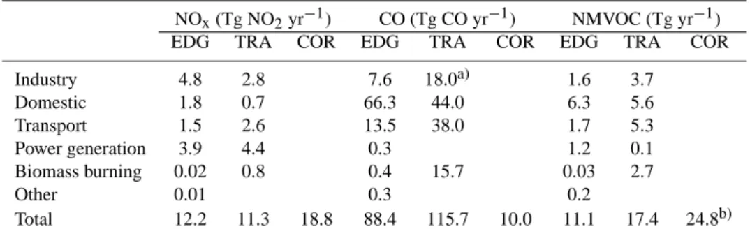
Table 1. Chinese emissions of NOx, CO and NMVOC as presented in the three independent emission inventory studies.
NOx(Tg NO2yr−1) CO (Tg CO yr−1) NMVOC (Tg yr−1)
EDG TRA COR EDG TRA COR EDG TRA COR
Industry 4.8 2.8 7.6 18.0a) 1.6 3.7 Domestic 1.8 0.7 66.3 44.0 6.3 5.6 Transport 1.5 2.6 13.5 38.0 1.7 5.3 Power generation 3.9 4.4 0.3 1.2 0.1 Biomass burning 0.02 0.8 0.4 15.7 0.03 2.7 Other 0.01 0.3 0.2 Total 12.2 11.3 18.8 88.4 115.7 10.0 11.1 17.4 24.8b)
Sources: Olivier et al. (2002) for EDGAR data (EDG), Streets et al. (2003) for TRACE-P data (TRA) and Bai (1996) for CORP data (COR). Sectional information for CORP is not available.a)Industry contains power generation emissions.b)NMVOC emissions have been estimated by using a NOx-NMVOC scaling factor.
construction. Gathering of these data is a time consuming task and in order to decide how much effort should be spent on the construction of an inventory, insight in the extent to which an inventory should be accurate is needed.
In this paper, results are presented of an analysis, which tests the sensitivity of a regional chemical transport model (Ma et al., 2002a) used to calculate summertime tropospheric ozone over China to the uncertainty in the anthropogenic
emission estimates of NOx, CO and NMVOC. The
princi-ple of this sensitivity run is that three independent emission inventories for China are used while keeping all other model settings (including non-Chinese emissions) constant.
2 Anthropogenic emission inventories
The used emission inventories are (i) emission estimates for the year 1995 from the Emission Database for Global Atmo-spheric Research (EDGAR v32; Olivier et al., 1999, 2002), (ii) regional emission inventory used in the Transport and Chemical Evolution over the Pacific (TRACE-P) program with emission estimates for the year 2000 (Streets et al., 2003) and (iii) national emission inventory used in the Chi-nese Ozone Research Programme (CORP) with emission es-timates for the year 1995 (Bai, 1996).
The inventories are different in (i) year for which emis-sions are calculated, (ii) level of detail that is included, (iii) information source for emission factors and activity data, and (iv) method of distributing emissions to (1◦×1◦) grid cells. The inventories share an important issue: due to the nature of emission factor calculations all inventories are known to be inaccurate representations of the emissions that have taken place in China over the year 1995. The extent to which the inventories are inaccurate is unknown. Furthermore, it is not assessed which inventory is the most accurate one.
2.1 The EDGAR v3 emission inventory
The EDGAR database presents a global estimate of several
compounds including NOx, CO, and NMVOC for the year
1990 and 1995 (Olivier et al., 1999, 2002). Emissions are calculated using an emission factor approach and emissions by sector are distributed on a 1◦×1◦ grid based mainly on population maps.
The methodology of EDGAR is described in detail in (Olivier et al., 1996, 1999, 2002). Activity data by coun-try – and thus for China – were taken from datasets compiled by international organizations which have performed consis-tency checks on the data. For example, energy data have been taken from the “Energy Statistics of OECD and non-OECD countries” (IEA/OECD, 1997) and industrial production data from “Industrial Commodity Production Statistics database” (UN, 1998). Applied emission factors are a mixture of emis-sion factors for groups of individual countries based on na-tional or regional studies and global default emission factors when no specific information was available. For China, most emission factors for NOx, CO and NMVOC are global or
re-gional default factors taken from the literature (Olivier et al., 2002 and references therein). Examples of country specific factors are those for CO and NOxfrom coalmine fires.
2.2 The TRACE-P emission inventory
As input for the TRACE-P project, Streets et al. (2003) have constructed a regional emission inventory for Asia with an-nual total emissions by country representing emission esti-mates for the year 2000. Emissions of several compounds, including NOx, CO and NMVOC are calculated on the
coun-try level. Chinese emissions are calculated by province. Emissions of NMVOC are further specified into 6 categories. The data used consist of actual statistical data for the year 2000, model forecasts values based on 1995 values and trend extrapolations from emission estimates for the late 1990’s. For China, activity data have been taken from
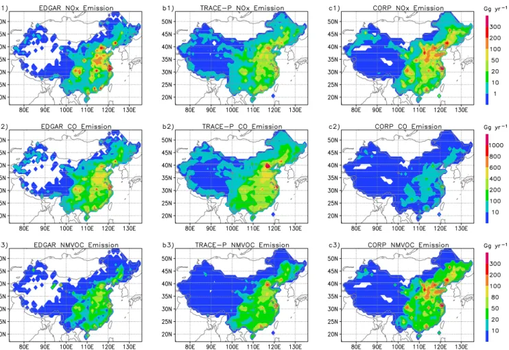
Fig. 1. Anthropogenic surface emissions of NOx, CO, NMVOC over China according to the EDGAR, TRACE-P and CORP estimates. Both
EDGAR and CORP estimates are for the year of 1995, and TRACE-P is for the year of 2000. While EDGAR and TRACE-P NMVOC emissions are independent on NOxemissions, CORP NMVOC emissions are scaled to NOxemissions. Units are Gg yr−1per 1◦×1◦grid.
country specific studies. For example, fuel use by sector and province were taken from by Sinton and Fridley (2000). Emission factors were applied both from studies on China (e.g. vehicle emission factors from Fu et al., 2001) and from global studies (e.g. biomass burning factors from Andreae and Merlet, 2001). Emissions by sector are distributed on 1◦×1◦grid cells based on population maps but also on for example road network maps.
2.3 The CORP emission inventory
For the CORP programme, Bai (1996) has calculated an emission inventory for China with NOx emissions represen-tative for the year 1992. This inventory has been updated for the year 1995 with CO emissions added. Unfortunately, this update has not been published. NMVOC emissions were not included in the CORP emission inventory. For modelling purposes, Ma et al. (2002a) added NMVOC emissions us-ing a NOx/NMVOC factor based on Berntsen et al. (1996).
These NMVOC emissions of Ma et al. (2002a) are used
for the inventory. The NOxemissions have been calculated
based on emission factors measured in China (Bai, 1996). For CO emissions, the source of information is unknown. Activity data have been taken from a variety of information sources on either State, Province and city level (Bai, 1996 and references therein). In general, energy statistics were available on at least the province level and for one fourth of the provinces data was available on the prefecture level. Ac-tivity data on industrial processes was taken from Ministerial yearbook publications. The calculated emissions were dis-tributed on a 1◦×1◦grid by dividing emissions by prefecture area. For grid boxes that contain more than one prefecture, the emission in the grid is averaged using weighted emission values.
2.4 Differences between emission inventories
Table 1 presents a summary of the emission estimates for
Chinese NOx, CO and NMVOC with Fig. 1 presenting the
Fig. 2. Difference in surface NOx, CO and CH2O due to the use of different emission inventories EDGAR, TRACE-P and CORP (denoted
as cases B, C1 and C2, respectively). Simulated results with EDGAR are given as reference and the differences are shown with the relative deviations of TRACE-P and CORP to EDGAR. Note that the relative differences are large for NOxin western China due to low emissions
and concentrations of NOxin unpolluted areas.
range from 11 Tg (TRACE-P) to 19 Tg (CORP) with the CORP inventory being about 50–60% higher than both the EDGAR and TRACE-P work. Although the EDGAR and
TRACE-P NOx budget are comparable (∼10%), large
dif-ferences can be seen in sector emissions. For the CORP in-ventory, no sector information is available. CO emissions range from 10 Tg (CORP) to 116 Tg (TRACE-P). EDGAR and TRACE-P emissions differ by 30% while the CORP val-ues seem unrealistically low. Again, EDGAR and TRACE-P show large sector differences. For example, transport emis-sions in EDGAR are 1/3 of the TRACE-P estimate while do-mestic emissions in EDGAR are twice the TRACE-P value. NMVOC emissions range from 11 Tg (EDGAR) to 25 Tg (CORP) with 45% difference between TRACE-P and the other inventories. Emissions by sector between EDGAR and TRACE-P show large differences, except for domestic emis-sions.
The distribution of emissions (Fig. 1) shows a common feature between the inventories with low emissions in west-ern China and high emissions in the east. In contrast with
TRACE-P and CORP, EDGAR assigns zero emissions to western China (Tibetan Plateau). The distribution of NOx
emissions show higher peak values by EDGAR and CORP with more equal distribution values of TRACE-P. For exam-ple, the Shanghai region shows value >300 Gg per year in EDGAR and CORP while TRACE-P shows values of 100–
200 Gg per year. For CO emissions, CORP shows very
low CO values (100–200 Gg in eastern China) in compari-son with the >200 Gg values in EDGAR and TRACE-P in-ventories. As with the NOx emissions, the distribution of
NMVOC emissions show higher values in the CORP inven-tory (200–300 Gg) in comparison with the more equally dis-tributed emissions within the EDGAR and TRACE-P inven-tories.
As shown above significant differences are observed be-tween the three emission inventories. Based on the available information it cannot be assessed which inventory provides the most accurate emission estimate for the year 1995. In general the following can be stated:
– EDGAR: emission estimates at higher aggregation
lev-els than the other inventories (both budget and grid). However, calculations are representative for the year 1995 and based on international datasets.
– TRACE-P: rather detailed emission inventory, which
has used detailed geographical maps to distribute the emissions. However, emissions are not representative for the year 1995.
– CORP: emission calculations at detailed prefecture
level in China (budget and grid). Emissions are rep-resentative for the year 1995 and emission factors based on local measurements have been used. However, doc-umentation of the inventory is insufficient.
3 Regional ozone modelling
The model used in this study is a 3-D regional chemical trans-port model (Ma et al., 2002a), which is extended from the Re-gional Acid Deposition Model (RADM) and aimed at study-ing the distribution and budget of tropospheric ozone and its precursors over China. The model domain covers China with a horizontal resolution of 100 km. In the vertical, the model extends up to pressure levels of 10 mbar for meteorological simulations and to the local thermal tropopause for chem-ical integration. The meteorologchem-ical fields for the model run are provided with the Fifth-Generation NCAR/Penn State Mesoscale Model (MM5). The chemical gas-phase mechanism in the model was initially developed by Stock-well (1986), and modified by updating the rate constants, in-troducing the effective photodissociation of ozone, incorpo-rating the permutation reactions of organic peroxy radicals, and replacing the lumped NO3+N2O5 reaction rate
expres-sions with the explicit ones (Ma et al., 2000). The revised chemical mechanism was well compared with the explicit NCAR’s Master Mechanism using the trace gas concentra-tions observed at the China regional background atmospheric observatory as model initial conditions. The mechanism was further improved by adding acetone as a tracer into the model and including parameterization of heterogeneous reactions of N2O5and NO3on sulfate aerosols (Ma et al., 2002a). The
model implemented with this mechanism was used for the study of tropospheric ozone over China by Ma et al. (2002a, b). In addition to updated anthropogenic surface emissions, natural NMVOC emissions, aircraft emissions and lightning NOx sources are taken into account. The initial fields and
lateral boundary condition for most chemical traces are pro-vided with a global chemical transport model for ozone and related chemical tracers (MOZART).
The three emission inventories have been implemented into the model followed by a sensitivity run for each inven-tory. The model simulation is performed for a summertime period, 1–15 July 1995 over which the results are averaged and analyzed. While different emission inventories are used
for China, the EDGAR inventory was applied for other coun-tries in the model domain in all simulations. Since all other model settings are kept constant, the difference in simulated ozone will be due to various independent emission inven-tories for China. The model sensitivity has been tested for (i) ozone precursor concentrations, (ii) net ozone production, (iii) ozone concentrations, (iv) validation of the model us-ing Global Atmospheric Watch (GAW) measurements and (v) exceedance of ozone standards.
3.1 Ozone precursor concentrations
Figure 2 presents the difference in calculated NOx, CO and
CH2O for the three model simulations. For illustrative
pur-poses, the model results using the EDGAR emission esti-mates for China are shown as a base case (Fig. 2a). The model results using TRACE-P (case C1) and CORP (case C2) are presented as deviations from this reference case (case B). Selection of the EDGAR emission inventory as refer-ences is arbitrarily based on the fact that it is widely used in atmospheric modelling. It does however not imply that it is better than the other inventories.
In much of the troposphere, ozone production is limited
by the abundance of NOx (WMO, 1995). In China, most
NOx emissions are confined in the boundary layer near the
surface (Ma et al., 2002a), which are mainly from fossil fuel combustion. Figure 2a1 presents surface NOxconcentrations
calculated using EDGAR. Due to the short lifetime, high NOxconcentrations are found in areas with large NOx
emis-sions. High NOxconcentrations of 3–9 ppbv are found in the
eastern and middle part of China. Low NOxconcentrations
are found in the western China, notably around the Tibetan Plateau. Peak values of NOx(>9 ppbv) can be seen around
the Chengdu, Shanghai and Beijing areas.
The relative differences between the reference case and the calculations using TRACE-P and CORP are shown in Figs. 2b1 and c1, respectively. Large differences in NOx
con-centrations will be found in areas where emissions are differ-ent (see Fig. 1). These differences are visible in North China (including Beijing and Shijiazhuang), Northeast China (in-cluding Shengyuang and Haerbin) as well as in the Sichuan Basin (including Chengdu and Chongqing) and East China regions (including Shanghai and Nanjing). Both TRACE-P and CORP simulations show up to 200% higher NOx
concen-trations in the low emission areas in the western and north-ern parts of China. These differences appear to be larger in western China for TRACE-P, while the CORP simulation re-sults in large difference with EDGAR in Northeast China. In the areas in Central and Eastern China with large emissions, the EDGAR simulation results in 20–100% higher NOx
con-centrations than TRACE-P and CORP. The difference can be around 3 ppbv or higher which is comparable to the NOx
levels in the polluted rural areas of East Asia (WMO, 1995). The primary source of CO is estimated to come predomi-nantly from anthropogenic origin. In addition, the oxidation
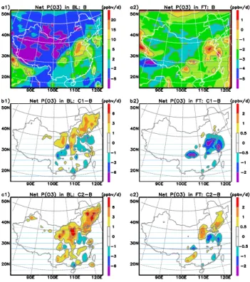
Fig. 3. Differences in calculated net production of ozone, P(O3), for the boundary layer (BL) and the free troposphere (FT) due to the use of different emission inventories EDGAR, TRACE-P and CORP (denoted as cases B, C1 and C2, respectively). Simulated results with EDGAR are given as reference and the differences are shown with the deviations of TRACE-P and CORP to EDGAR.
of CH4and NMVOC provide an important secondary source
of CO in the atmosphere (Von Kuhlmann, 2001). In the EDGAR simulation (Fig. 2a2) higher CO concentrations (>400 ppbv) are found in eastern China and lower concen-trations in the west. Peak CO concenconcen-trations (700–900 ppbv) are found in the Chengdu area of the Sichuan Basin, a larger area of North China below Beijing and a small area
of East China near Shanghai. While CO concentrations
from the TRACE-P simulation are comparable with EDGAR (Fig. 2b2), CO concentrations from the CORP simulation show values of up to 100% lower in eastern China.
Since NMVOC includes many species that are involved in the oxidation reactions for ozone formation (Atkinson, 2000), lumped NMVOC species are used for the purpose of simplification and efficient calculation of the model (Ma et al., 2002a). Therefore, it is not convenient to compare the results with observations or other model studies if the
concentrations of total NMVOC are presented.
Propene-equivalent NMVOC was used to analyze the relationship be-tween ozone and its precursors in Chameides et al. (1992). In this paper distribution of CH2O are shown. As shown in
Fig. 2a3, CH2O concentrations follow the pattern of NOxand
CO concentrations (Figs. 2a1, a2). In the regions with high emissions the EDGAR and TRACE-P simulations (Fig. 2b3)
show comparable concentrations. In low emission areas, the results from TRACE-P show larger CH2O concentrations.
The difference between the EDGAR and CORP simulations
is rather large. The CORP simulations show differences
larger 200% in North and Northeast China.
3.2 Net ozone production
Figure 3a shows the net ozone production for the boundary layer (Fig. 3a1) and free troposphere (Fig. 3a2) as calculated in the EDGAR simulation. The largest net ozone production values are found in the polluted regions of eastern China, with maximum values of 10–15 ppbv/day. Figures 3b and c show the differences between the EDGAR and the TRACE-P and CORTRACE-P simulations. In general, the CORTRACE-P simulation results in higher net ozone production in the boundary layer, especially in North and Northeast China. The largest differ-ences are up to 6 ppbv/day, which is nearly 30–50% of maxi-mum net ozone production estimated for the polluted regions of eastern China (Mauzerall et al., 2000; Ma et al., 2002a). The EDGAR and TRACE-P simulations differ with higher net ozone production in Northeast China for TRACE-P and with higher values using EDGAR for the Sichuan Basin and East China regions. This difference is relatively small in comparison to the CORP simulation. In the free troposphere (Figs. 3a2, b2, c2) the difference in net ozone production is confined to limited regions, but its magnitude is still consid-erable, reaching to 1 ppbv/day or more in some regions.
3.3 Ozone concentrations
Figure 4 presents simulated O3concentrations at the surface
(4a1) and at 500 mbar height (4a2) using the EDGAR inven-tory together with differences with the TRACEP (4b1, b2) and CORP (4c1, c2) simulations. High O3 concentrations
are found in Central east and Northeast China and on the Ti-betan plateau where altitudes fall in the middle troposphere. For surface ozone, the differences occur mainly in Northeast China and the East China Sea. Both the CORP and TRACE-P simulations result in ozone concentrations with the differ-ence reaching up to 50% at some locations (e.g. Shanghai area) but in general the differences are less than 30%. Dif-ferences in ozone concentration at 500 mbar show a different pattern. Here the differences occur over the Sichuan Basin, East China and its down-stream regions over the sea. This corresponds to the corridor where O3 is predominantly
at-tributed to photochemistry (Ma et al., 2002b). The EDGAR simulations show slightly higher values (up to 5%) than the
TRACE-P simulation. Results from CORP and EDGAR
are comparable, except for the Guizhou area with up to 3% higher concentrations in the CORP simulation.
The reasons for the smaller difference in simulated ozone concentration than in its precursors, for instance, NOx, are
complicated. In unpolluted areas (e.g. western China), an-thropogenic NOxemissions as well as its concentrations are
Fig. 4. Differences in simulated O3at the surface and 500 mbar height due to the use of different emission inventories EDGAR, TRACE-P and CORP (denoted as cases B, C1 and C2, respectively). Simulated results with EDGAR are given as reference and the dif-ferences are shown with the deviations of TRACE-P and CORP to EDGAR.
low, and ozone is controlled mainly by the transport (Ma et al., 2002b). The differences in NOxemissions as well as its
concentrations may be rather larger in relative sense. How-ever, the differences in simulated ozone concentrations are smaller due to rather small fraction of ozone attributed to in situ photochemistry. In polluted areas (e.g. most parts of eastern China), anthropogenic NOxemissions as well as its
concentrations are high, and ozone is controlled mainly by photochemistry (Ma et al., 2002b). Ozone concentrations should be sensitive to the variations in NOxconcentrations
and thus its emissions. However, the amount of ozone pro-duced per NOxemitted is not linear (Liu et al., 1987; Lin et
al, 1988; Trainer et al., 1993). With NOxozone production
increases at high NOxlevels and decreases at high NOx
lev-els, and the NOxthreshold is around 1–10 ppbv, depending
on NMVOC conditions and so on (Poppe et al., 1998). Gen-erally, surface NOxlevels in polluted areas of eastern China
fall in this range (Fig. 2a1). Therefore, the differences in simulated ozone vary and can be opposite in sign with the differences in simulated NOx(Figs. 2b1, 3b1 and 4b1).
Ka-sibhatla et al. (1998) estimated that the net ozone production efficiency (OPE) ranges from 2 to 3 ppbv O3ppbv−1NOxin
the eastern United States during summer. Assuming a 100% NOxincrease at 3 ppbv NOxand 30 ppbv O3, the O3increase
Fig. 5. Differences in simulated surface O3due to the use of
differ-ent emission rates of EDGAR, TRACE-P and CORP for a specific species while keeping rest the same as those of EDGAR. The sim-ulated result with EDGAR is taken as reference, which is given in Fig. 4a1. The differences are shown with the relative deviations to EDGAR when TRACE-P NOx, CO and NMVOC (denoted as S1,
S3 and S5) and CORP NOx, CO and NMVOC (denoted as S2, S4
and S6) are used, respectively.
is estimated to be 6 to 9 ppbv, i.e. 20–30% increase in rela-tive sense. Our results are in agreement with this estimate, indicating that the model chemical mechanism we used is re-liable.
To determine whether it is the combination of different emission estimates or the difference in one species that controls the difference in ozone concentrations, additional model simulations were performed which are discussed here briefly. The model sensitivity runs were performed with the scenarios below, where EDGAR emissions were replaced with TRACE-P or CORP for one species.
S1: TRACE-P NOxwith EDGAR CO and NMVOC;
S2: CORP NOxwith EDGAR CO and NMVOC;
S3: TRACE-P CO with EDGAR NOxand NMVOC;
S4: CORP CO with EDGAR NOxand NMVOC;
S5: TRACE-P NMVOC with EDGAR NOxand CO;
S6: CORP NMVOC with EDGAR NOxand CO.
Differences in simulated surface O3due to the use of these
scenarios are compared with the reference simulation using the EDGAR emission inventory for all species.
0 4 8 12 16 20 24 40 50 60 70 80 O3 (p pbv) 0 4 8 12 16 20 24 0 10 20 30 40 O3 (p pbv) 0 4 8 12 16 20 24 Local Time (hr) 0 10 20 30 40 50 60 O3 (p pbv) a) Waliguan b) Lin'an c) Longfengshan CORP EDGAR TRACE-P
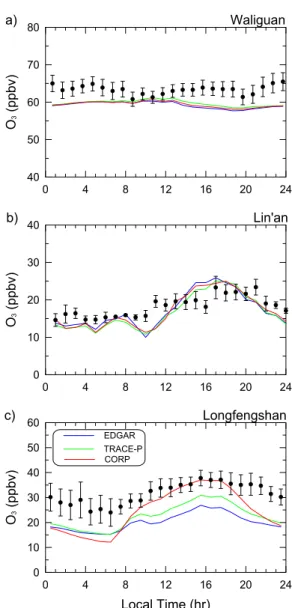
Fig. 6. Simulated mean diurnal cycles of surface O3 at the
three WMO/GAW background stations Mt. Waliguan, Lin’an and Longfengshan for different emission inventories EDGAR, TRACE-P and CORTRACE-P (denoted as blue, green and red lines, respectively). Observations (circles, with bars for standard deviations) are also shown for comparison. The geographic position of the stations is given in Fig. 4a1 and denoted by A, B and C for Mt. Waliguan, Lin’an and Longfengshan, respectively.
As shown in Fig. 5a1, the difference between EDGAR and TRACE-P (Fig. 4a1) is caused dominantly by the difference in NOx emissions, in addition, partly by the difference in
NMVOC emissions (Fig. 5c1). The difference in the CO emission between EDGAR and TRACE-P has little effect on simulated surface O3(Fig. 5b1). The difference between
CORP and EDGAR (Fig. 4c1) is caused by the combined effect of difference in the emission of NOx (Fig. 5a2), CO
(Fig. 5b2) and NMVOC (Fig. 5c2). This effect, however, is not a simple addition of the emission differences but is an effect of the non-linear characteristics of ozone chemistry.
3.4 Diurnal variation of ozone at GAW stations
Measurements of ozone and its precursors are sparse in China, especially in the rural areas. Surface ozone was ob-served at the three WMO Global Atmosphere Watch (GAW) background stations in the CORP programme (Zhou, 1996). Figure 6 presents the simulated mean diurnal cycles of O3at
stations Mt. Waliguan (WLG), Lin’an (LA) and Longfeng-shan (LFS). The location of these stations is shown in Fig. 4a1 with markings A (WLG), B (LA) and C (LFS). Sim-ulated daily variations of O3at the WLG and LA stations do
not show large difference between the three simulations. The differences between the simulations and observation are rel-atively small with a good fit at LA and with some underesti-mation at WLG station.
As can be expected, simulated O3 at WLG stations is
nearly the same for all three simulations. The source of O3
at WLG is mainly from long-range transport outside China (Ma et al., 2002b). The sources of O3at LA are both from
photochemistry inside and transport outside China (Ma et al., 2002b). The close agreement between the simulation at LA are due to the small differences in emission estimates for the rural areas of south China and dominating sea winds. Sim-ulated daily O3variations at LFS stations show different
re-sults. While the CORP simulation reproduces observed O3
during the day, there is an underestimation for both EDGAR and TRACE-P calculations. Because LFS is in the summer downstream of polluted areas, the emission inventory differ-ences in Northeast and North China might contribute to the differences found at this station.
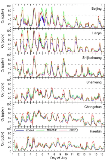
3.5 Exceedance of ozone standards in selected grid cells As shown in Fig. 4, differences in simulated surface O3are
large in North and Northeast China. This could have im-plications for studying ozone exceedance in major cities in that area. Figure 7 presents the hourly O3 variation in
se-lected model grid cells where six large cities in North and Northeast China are located. The government of China has set several ozone standards of which the first level standard of 60 ppbv hourly maximum has been applied. Although the size of model grid cell is not small enough to resolve a city, the simulated results can be an indicator of air quality al least for the regions where these cities are. As shown in Fig. 7, several cities show an exceedance of this standard, es-pecially in the first days of the simulation period. For the city of Beijing and Tianjin, it is clearly visible that the EDGAR simulation does not lead to exceedance of the ozone stan-dard while the TRACE-P and CORP simulations result in exceedance during several days. The maximum difference in hourly-averaged ozone concentration can reach up to 40 ppbv or 100% in relative sense. For the other cities, ozone concen-trations rarely exceed the standard, but the relative deviation due to different emission inventories is still high sometimes with a maximum of near 100%.
4 Conclusions
In this paper the sensitivity of simulated ozone to different emission inventories of ozone precursors has been studied. Three independent emission inventories (EDGAR, TRACE-P and CORTRACE-P) with emission estimates for NOx, NMVOC and
CO in China have been used as input for simulations with a regional chemical transport model (Ma et al., 2002a).
Large differences were found in the simulated precursor
concentrations. For both NOxand NMVOC the EDGAR
cal-culations resulted in lower concentrations in the northern part of China. For NOx these differences are up to 200% while
for NMVOC these differences are up to 100% in comparison with TRACE-P and up to 200% with CORP. Simulation of CO concentrations using EDGAR and TRACE-P are compa-rable with differences of about 20%. The CORP simulation results in significant lower CO concentrations (up to 100%) than the other simulations. These differences are most likely caused by the different CO emission budgets with CORP es-timating 5–6 lower CO emissions than the other two inven-tories.
Although large differences were found in the precursor concentrations and significant differences occurred in the boundary layer net ozone production values, the differences in ozone concentrations are relatively small for a regional ozone model. Differences in surface ozone occurred mainly in North and Northeast China with as well as in the East China Sea. Both CORP and TRACE-P simulations showed higher ozone concentrations than the EDGAR simulations with differences of up to 50% in the Shanghai and Beijing area. For most of the model domain, however, differences are only 5–30%. Differences in O3at 500 mbar occur mainly
over the Sichuan Basin, North China and its down-stream re-gions over the sea, with maximum differences of 1–2 ppbv (less than 5%). Application of TRACE-P generally resulted in lower O3values at 500 mbar in comparison with EDGAR
and CORP.
The results from additional local simulations in which one species from the TRACE-P and CORP emission inven-tory was mixed with the EDGAR estimates for the other species showed that the difference between TRACE-P and the EDGAR simulations can be attributed mainly to the NOx
emission inventory differences, less to NMVOC and not to CO emission inventory differences. Given the discussion above on precursor concentrations, the difference in ozone calculations between EDGAR and TRACE-P are mainly re-lated to the difference in distribution of the NOxemissions.
The differences between EDGAR and CORP ozone calcu-lations is less clear and seems to be the combined effect of differences in NOx, CO and NMVOC emissions.
The main purpose of this paper is to discuss to what ex-tent uncertainty in regional emission inventories really mat-ters for the outcome of atmospheric modelling studies.
As far as surface O3in rather unpolluted areas and O3at
higher altitudes (500 mbar) are concerned, the different
sim-0 20 40 60 80 100 O 3 (p pbv ) 0 20 40 60 80 100 O 3 (p pbv ) 0 20 40 60 80 100 O 3 (p pbv ) 0 20 40 60 80 100 O 3 (p pbv ) 0 20 40 60 80 100 O 3 (p pbv ) 1 2 3 4 5 6 7 8 9 10 11 12 13 14 15 16 Day of July 0 20 40 60 80 100 O 3 (p pbv ) Beijing Tianjin Shijiazhuang Shenyang Changchun Haerbin CORP TRACE-P EDGAR
Fig. 7. Simulated hourly variations of surface O3 for the
se-lected model grid cells with different emission inventories EDGAR, TRACE-P and CORP (denoted as blue, green and red lines, re-spectively). The grid cells are denoted with the name of big cities which are included in the grid cells. The first-level ozone standard (60 ppbv) is shown with black dashed lines.
ulations show that the application of different emission in-ventories did not result in significant differences. For the higher altitudes, photochemistry and atmospheric transport play a more important role than the variation (uncertainty) in surface emissions. For the unpolluted areas, the relative dif-ferences in the emission inventories were found to be large but due to the low emissions values this does not have a large effect on simulated ozone values.
As far as surface O3 in polluted areas is concerned, the
results show that 30–50% differences in ozone concentra-tions values were found. Maximum differences of 10 ppbv were found in the region where the big cities of Beijing and Tianjin are located. Although the inventories show large dif-ferences, regional modelling of ozone shows concentrations within 30–50% which – at first sight – does not seem very large for this type of modelling, especially when the emis-sion inventories show large differences.
For more localized studies, for which the model suitabil-ity could be questioned, significant differences were ob-served. In the area where maximum differences (10 ppbv) were found, ozone levels in Beijing and Tianjin were above the exceedance level in the TRACE-P and CORP calcula-tions while the EDGAR calculacalcula-tions did not lead to ex-ceedance. In this case the difference in emission inventories did matter. In addition, the comparison of the diurnal O3
cy-cles with the measurements made at a WMO/GAW regional background station, the Longfengshan station, was depen-dent on which emission inventory was used for the model calculation.
In the opinion of the authors, a difference of 30–50% in simulated ozone values, between model calculations using either a (i) inventory of high aggregation level with several global default emission factors, (ii) detailed inventory with emissions not representative for 1995 and (iii) detailed inven-tory of NOxemissions with unknown method for CO and a
scaling of NOxemissions to reach NMVOC estimates, is not
extremely large. In this perspective the uncertainty in emis-sion inventories does not lead to important different insights and the strain on emission inventories being the limitation in regional ozone modelling seems to be unjustified, especially when meteorological variations or chemical reactions within the model could also lead to large variation in the model out-come.
Finally, a question to be answered is which inventory should be used for simulating summertime ozone in China in 1995? If the measurements at the Longfenshang station in Northeast China are used as an indicator, one should have more confidence in the CORP emission inventory than in the EDGAR and TRACE-P emission inventories. However, given its large underestimation of CO emission values this confidence seems to be misplaced. In general, there is no confidence to highlight which emission inventory is better than the other at the present time. Either a detailed compar-ison of methodology of the three emission inventories or the availability of more measurements to validate the model re-sult could provide this insight. Unfortunately, this is not pos-sible due to lack of documentation on the CORP inventory and the limited amount of measurement data.
Acknowledgements. The authors would like to thank M. Lawrence and J. Lelieveld for their comments and suggestions on this work. J. Ma also acknowledges the support of MOST under the project 2002DIA20012. Special thanks go to the START Visiting Scientist Programme for supporting J. Ma’s visit to the Max Planck Institute for Chemistry.
Edited by: A. Guenther
References
Andreae, M. O. and Merlet, P.: Emissions of trace gases and aerosols from biomass burning, Global Biogeochemical Cycles, 15, 955–966, 2001.
Atkinson, R.: Atmospheric chemistry of VOCs and NOx, Atmo-spheric Environment, 34, 2063–2101, 2000.
Bai, N. B.: The emission inventory of CO2, SO2, and NOxin China,
in The Atmospheric Ozone Variation and Its Effect on the Cli-mate and Environment in China, edited by Zhou, X. J., 145–150, Meteorological Press, Beijing (in Chinese), 1996.
Berntsen, T., Isaksen, I. S. A., Wang, W.-C., and Liang, X.-Z.: Impacts of increased anthropogenic emissions in Asia on tropo-spheric ozone and climate: A global 3-D model study, Tellus, 48B, 13–32, 1996.
Chameides, W. L, Fehsenfeld, F., Rodgers, M. O., Cardelino, C., Martinez, J., Parrish, D., Lonneman, W., Lawson, D., Ras-mussen, R., Zimmerman, P., Greenberg, J., and Middleton, P.: Ozone precursor relationships in the ambient atmosphere, J. Geo-phys. Res., 97 (D5), 6037–6055, 1992.
Fu, L., Hao., J., He, D., He, K., and Li, P.: Assessment of vehic-ular pollution in China, Journal of Air and Waste Management Association, 51, 658–668, 2001.
IEA/OECD: Beyond 20/20, Release 4.1, Energy balances of OECD countries, Energy balances of Non-OECD countries, Ivation DatasystemsInc, 1997.
Kasibhatla, P., Chameides, W. L., Saylor, R. D., and Olerud, D.: Relationships between regional ozone pollution and emissions of nitrogen oxides in the eastern United States, J. Geophys. Res., 103, 22 663–22 669, 1998.
Lin, X., Trainer, M., and Liu, S.: On the nonlinearity of tropo-spheric ozone production, J. Geophys. Res., 93, 15 879–15 888, 1988.
Liu, S., Fehsenfeld, F., Parrish, D. D., Williams, E., Fahey, D. W., Huebler, G., and Murphy, P.: Ozone production in the rural tro-posphere and the implications for regional and global distribu-tions, J. Geophys. Res., 92, 4191–4207, 1987.
Ma, J., Li, W. L., and Zhou, X. J.: Improvements of RADM1 gas phase chemical mechanism, J. Environ. Sci. Health, A35, 1931– 1939, 2000.
Ma, J., Liu, H., and Hauglustaine, D.: Summertime tropospheric ozone over China simulated with a regional chemical transport model, Part 1. Model description and evaluation, J. Geophys. Res., 107 (D22), 4660, doi:10.1029/2001JD001354, 2002a. Ma, J., Zhou, X., and Hauglustaine, D.: Summertime tropospheric
ozone over China simulated with a regional chemical transport model, Part 2. Source contribution and budget, J. Geophys. Res., 107 (D22), 4612, doi:10.1029/2001JD001355, 2002b.
Mauzerall, D. L., Narita, D., Akimoto, H., Horowitz, L., Walters, S., Hauglustaine, D. A., and Brasseur, G.: Seasonal character-istics of tropospheric ozone production and mixing ratios over East Asia: A global three-dimensional chemical transport model analysis, J. Geophys. Res., 105, 17 895–17 910, 2000.
Olivier, J., Bouwman, A. F., Van der Maas, C. W. M., Berdowski, J. J. M., Veldt, C., Bloos, J. P. J., Visschedijk, A. J. H., Zand-veld, P. Y. J., and Haverlag, J. L.: Description of EDGAR Ver-sion 2.0: A set of emisVer-sion inventories of greenhouse gases and ozone depleting substances for all anthropogenic and most nat-ural sources on a per country basis and on 1◦×1◦grid, RIVM Rep. 771060002, Bilthoven: National Institute of Public Health and the Environment, 1996.
Olivier, J. G. J., Bloos, J. P. J., Berdowski, J. J. M., Visschedijk, A. J. H., and Bouwman, A. F.: A 1990 global emission inventory of anthropogenic sources of carbon monoxide on 1◦×1◦
devel-oped in the framework of EDGAR/GEIA, Chemosphere: Global Change Science, 1, 1–17, 1999.
Olivier, J. G. J, Peters, J. A. H. W., Bakker, J., Berdowski, J. J. M., Visschedijk, A. J. H., and Bloos, J. P. J.: Applications of EDGAR: emission database for global atmospheric research, Re-port no.: 410.200.051. RIVM, The Netherlands, 2002.
Pacyna, J. M. and Graedel, T. E.: Atmospheric emission invento-ries: status and prospects, Annual review of energy and the envi-ronment, 20, 265–300, 1995.
Poppe, D., Koppmann, R., and Rudolph, J: Ozone formation in biomass buning plumes: Influence of atmospheric dilution, Geo-phys. Res. Lett., 25, 3823–3826, 1998.
Russell, A. and Dennis, R.: NARSTO critical review of photochem-ical models and modelling, Atmos. Environ., 34, 2283–2324, 2000.
Sintion, J. E. and Fridley, D. G.: What goes up: recent trends in China’s energy consumption, Energy and Policy, 28, 671–687, 2000.
Stockwell, W. R.: A homogeneous gas-phase mechanism for use in a regional acid deposition model, Atmos. Environ., 20, 1615– 1632, 1986.
Streets, D. G., Bond, T. C., Carmichael, G. R., Fernandes, S. D., Fu, Q., He, D., Klimont, Z., Nelson, S. M., Tsai, N. Y., Wang, M. Q., Woo, J.-H., and Yarber, K. F.: An inventory of gaseous and primary aerosol emissions in Asia in the year 2000, J. Geophys. Res., 108 (D21), 8809, doi:10.1029/2202JD003093, 2003.
Trainer, M., Parrish, D. D., Buhr, M. P., Norton, R. B., Fehsenfeld, F. C., Anlauf, K. G., Bottenheim, J. W., Tang, Y. Z., Wiebe, H. A., Roberts, J. M., Tanner, R. L., Newman, L., Bowersox, V. C., Meagher, J. F., Olszyna, K. J., Rodgers, M. O., Wang, T., Berresheim, H., Demerjian, K. L., and Roychowdhury, U. K.: Correlation of ozone with NOy in photochemically aged air, J. Geophys. Res., 98, 2917–2925, 1993.
United Nations (UN): Industrial commodity production statistics 1970–1995. UN Statistical Division, New York, Data file re-ceived 30-1-1998.
Van Aardenne, J. A., Carmichael, G. R., Levy, H., Streets, D., and Hordijk, L.: Anthropogenic NOxemissions in Asia in the period
1990–2020, Atmos. Environ., 33, 633–646, 1999.
Von Kuhlmann, R.: Tropospheric photochemistry of ozone, its pre-cursors and hydroxyl radical: A 3-D modeling study considering non-methane hydrocarbons, Ph.D thesis, University of Mainz, Mainz, Germany, 2001.
World Meteorological Organization (WMO): Scientific Assessment of Ozone Depletion: 1994, Global Ozone Research and Monitor-ing Project, Rep. 37, Geneva, Switzerland, 1995.
Zhou, X. J. (Ed.): The Atmospheric Ozone Variation and Its Effect on the Climate and Environment in China, Meteorological Press, Beijing (in Chinese), 1996.