An Augmented Lagrangean Approach for the QoS Constrained Routing Problem

(1)

HAL Id: hal-00678369

https://hal.archives-ouvertes.fr/hal-00678369

Submitted on 12 Mar 2012

HAL is a multi-disciplinary open access

archive for the deposit and dissemination of sci-entific research documents, whether they are pub-lished or not. The documents may come from teaching and research institutions in France or abroad, or from public or private research centers.

L’archive ouverte pluridisciplinaire HAL, est destinée au dépôt et à la diffusion de documents scientifiques de niveau recherche, publiés ou non, émanant des établissements d’enseignement et de recherche français ou étrangers, des laboratoires publics ou privés.

An Augmented Lagrangean Approach for the QoS

Constrained Routing Problem

Christophe Duhamel, Antoine Mahul

To cite this version:

Christophe Duhamel, Antoine Mahul. An Augmented Lagrangean Approach for the QoS Constrained Routing Problem. 2007. �hal-00678369�

(2)

An Augmented Lagrangean Approach for the QoS Constrained Routing Problem

Christophe Duhamel1_{, Antoine Mahul}2

LIMOS, UMR 6158-CNRS

Universit´e Blaise-Pascal, BP 10125, 63173 Aubi`ere, France. Research Report LIMOS/RR07-15

1_{christophe.duhamel@isima.fr}

(3)

Abstract

Given a directed graph with capacities on each arc and given a set of commodities, the QoS constrained Routing Problem (QCRP) consists in routing each commodity while respecting a end-to-end upper bound on the delay for each packet. This problem is NP-hard and we propose an augmented Lagrangean approach to solve it. A flow deviation algorithm as well as a projected gradient method are proposed to solve the inner problem in the augmented Lagrangean approach. The delay and the load functions are approximated either by an analytical function or by a neural network. Computational results are reported to show the effectiveness of the projected gradient method and the neural network approximation.

Keywords: routing, quality of service, nonlinear programming, augmented Lagrangean, flow deviation, projected gradient, neural network

R´esum´e

Étant donné un graphe muni de capacités sur les arcs ainsi qu’un ensemble de demandes, le problème de Routage avec Contraintes de Qualité de Service (QRCP) consiste à router chaque demande tout en respectant une borne supérieure sur le délai de bout en bout pour chaque paquet. Ce problème est NP-difficile et nous proposons une approche de type Lagrangien Augmenté pour le traiter. Nous proposons un algorithme de déviation de flot ainsi qu’une méthode de gradient pro-jeté pour résoudre le sous-problème à chaque itération du Lagrangien Augmenté. Nous utilisons deux types d’approximation pour les fonctions de délai et de charge sur les arcs : une fonction ana-lytique ou un réseau de neurones. Cette approche est testée sur des instances de taille réaliste. Les expérimentations montrent que l’utilisation de réseaux de neurones ainsi que du gradient projeté permettent d’obtenir de bons résultats dans des temps acceptables.

Mots clés : routage, qualité de service, programmation non linéaire, lagrangien augmenté, déviation de flot, gradient projeté, réseau de neurones

(4)

Introduction

The demand for a dynamic and efficient usage of network resources is one of the key points in the current evolution of the Internet. However, to support both existing and emerging (VoIP, peer-to-peer, ad-hod, etc.) multimedia applications with specific Quality of Service (QoS) requirements, additional services and protocols are needed. IETF has proposed several approaches to address QoS requirements in the Internet. DiffServ-based architectures have received the greatest favors of operators and in the industry but the deployment of end-to-end QoS is still limited [11]. Although the basic DiffServ concept (differenciation of packets per traffic classes) is being currently ex-ploited to support voice traffic over IP network (VoIP), handling the traffic in term of performance (delay, loss rate, jitter) is still an open issue [13].

One of the problems is to design effective routing policies that allow QoS constraints to be respected and ressource occupation to be optimized. MultiProtocol Label Switching (MPLS) is being considered as one (standardized) approach for scalable QoS provisioning in the Internet and may be seen as a possible answer to Traffic Engineering (TE) needs. We adress here the prob-lem of routing a set of demands in a MPLS backbone with QoS requirements expressed in term of end-to-end delays. The classical optimization algorithms that are typically used in TE task to maximize network performance and to balance traffic load suffer from a major issue: they still rely on the assumption that the QoS in routers obeys the standard M/M/1 formula. In this work, we define a multicommodity flow optimization procedure in which the M/M/1 approximation can be substituted by a more realistic evaluation of the delay using a neural network trained on simulated examples. We restrict ourselves to the QoS constraint defined as the end-to-end delay: for each commodity, it corresponds to the delay incurred by a packet between its arrival time at the desti-nation router and its departure time from the origin router. The QoS Contrainted Routing Problem (QCRP) is then to route each commodity on the network in order to minimize the overall load on the network – defined as the overall sum of the arc loads – while respecting all QoS require-ments. Note that a somewhat different cost function could have been used, namely the maximal congestion on the network (i.e. the utilization factor on the most saturated arc) as discussed in [7]. A mathematical formulation for (QCRP) is presented in Section 1. Then we describe in Sec-tion 2 an augmented Lagrangean approach to solve the problem. The subproblem reduces to a nonlinear minimum cost flow problem. It will be solved two different ways: first, by using the flow deviation method, second, by using the projected gradient method. Due to the nature of the objective function, the generation of the improving direction for both methods requires a specific algorithm. In Section 3, two approximations (the classical Kleinrock’s delay function and a neural network-based function) are presented for the delay and the load functions. Numerical results will be presented in Section 4 before concluding remarks.

1 Mathematical formulations

Let G = (N, A, c) be a directed network, where N is the set of nodes (routers) and A is the set of arcs (connections). A capacity (bandwidth) ca > 0 is associated with each arc a ∈ A. The set

of commodities (services) to be routed on G is defined as K = {(oi, di, qi, si), i = 1 . . . K}. For

each commodity k ∈ K, o_kis the origin node, d_kis the destination node, q_kand s_kare respectively the requested bandwidth and the class of service. The bandwidth requirement qkis considered to

be fixed, i.e. the traffic is not subject to variations over the time. The set S = {si, i = 1 . . . S}

contains the classes of service. To each class of service s ∈ S, D_s is the upper bound on the end-to-end delay. Thus, for every commodity k ∈ K, Dskcorresponds to the maximal end-to-end

(5)

Let Pk=

©

pk_i, i = 1 . . . Pk

ª

be the set of all paths for commodity k ∈ K. Thus, P = ∪k∈KPk

denotes the set of all the paths. Each path p ∈ P can be expressed as a set of arcs. For each commodity k, let xk

p > 0 be the percent of bandwidth assigned to the path p ∈ Pk. Throughout

this work, the delay will be considered as an additive function over the arcs. Therefore, the end-to-end delay for a path p ∈ P is given by the sum of the delays on each arc a belonging to p. Let φs(xa, ca) and ψs(xa, ca) be respectively the load function and the delay function for the class of

service s ∈ S on the arc a ∈ A, where xais the aggregated bandwidth vector for each class of

service. The (QCRP) can be formulated as follows:

(QCRP) Min Φ(x) =X a∈A X s∈S φs(xa, ca) s.t. X p∈Pk xk_p = 1 ∀k ∈ K (1) xs_a= X k∈K|sk=s qk X p∈Pk|a∈p xk_p ∀a ∈ A, ∀s ∈ S (2) dk_p = X a∈A|a∈p ψ_s_k(x_a, c_a) ∀k ∈ K, ∀p ∈ P_k (3) xk_p ³ D_s_k − dk_p ´ > 0 ∀k ∈ K, ∀p ∈ P_k (4) xk_p > 0 ∀k ∈ K, ∀p ∈ Pk

Constraints (1) require all the bandwidth to be assigned to the paths of commodity k. Equa-tions (2) compute the bandwidth used on each arc according to the bandwidth that is assigned on each path. Equations (3) compute the end-to-end delay of each path. Finally, constraints (4) are the QoS constraint for each active path, i.e. for each path on which a positive amount of bandwidth is routed. These constraints are nonlinear and nonconvex. It is worth noting that only (1) and (4) define constraints, since xs

aand dkp are auxiliary variables. Moreover, the capacity constraints are

not used in (QCRP) since the delay function ψs acts as a barrier on the arcs capacity. Thus, the

capacity constraints are redundant in our context. (QCRP) is NP-hard as shown by Ben-Ameur and Ouorou [1]. In fact, even the computation of a shortest path given several QoS metrics is NP-hard, as shown by [15]. To our knowledge, [1] is the only work trying to take the end-to-end delay constraint into account. They consider a minimum cost flow problem subject to QoS con-straints. They first give a mathematical model before proposing several lower and upper bounds by performing convexifications. No computational results are given, though.

2 Augmented Lagrangean method for (QCRP)

A wide range of efficient methods are well-suited to solve convex multicommodity minimum cost flow problems (see [14] for a comprehensive survey and comparison). Yet, most of them cannot be applied to this problem since the load and the delay functions, φs(xa, ca) and ψs(xa, ca), are

nonlinear. Moreover, there is an exponential number of nonlinear, nonconvex QoS constraints (4). Thus, they will be first dualized by performing a Lagrangean relaxation. Let gk

p(x) = xk p ¡ dk p − Dsk ¢

. Then the objective function becomes

(6)

L(x, λ) =X a∈A X s∈S φs(xa, ca) + X k∈K,p∈Pk λk_pgk_p(x) (1) where λk

p > 0 are the Lagrangean coefficients associated with each relaxed QoS constraint.

The resulting problem consists in minimizing the nonlinear objective function (1) with linear con-straints.

The Lagrangean relaxation cannot be solved directly as the objective function L(x, λ) is non-convex (due to g_pk(x)). An augmented Lagrangean relaxation scheme can be built by adding a quadratic penalty term to the objective function (see [6]). Let hk

p(x, λ, c) = max © 0, λk p+ cgpk(x) ª . Then the augmented Lagrangean function is

Lc(x, λ) = X a∈A X s∈S φs(xa, ca) + 1 2c X k∈K,p∈Pk µ³ hk_p(x, λ, c) ´₂ − ³ λk_p ´₂¶ (2) Lc(x, λ) is locally convex at the neighborhood of x and the resulting problem can be solved

by any classical optimization method (i.e. subgradient method, bundle method). At each itera-tion of the augmented Lagrangean method, the Lagrangean multipliers λ are fixed (λt) and the

subproblem (L+_c,t) to be solved is as follows:

(L+_c,t) Min Lc(x, λt) s.t. X p∈Pk xk_p = 1 ∀k ∈ K (1) xk p > 0 ∀k ∈ K, ∀p ∈ Pk

At iteration t, let x+_t be the solution of (L+_c,t). The multipliers are updated using the formula

λt+1= max{0, λt+ ctg(xt)} (3)

The multipliers method is applied on the QoS constraints removal (partial constraint removal). The remaining constraints are linear. This ensures the convergence of the method ([3, 8]). How-ever, as L(x, λ) is nonconvex, the augmented Lagrangean method converges towards a local op-timum. Thus, the computed solution x∗ is only a local optimum. However, this solution is still interesting for two reasons: first, it is feasible, especially with respect to the QoS constraints. Moreover, a lower bound can be computed within the method. This will give us an estimation of the quality of our primal solution.

The choice for the serie {ct} is derived from [6]. It consists in multiplying ctby a constant

factor β (here β = 10) each time the overall violation of the QoS constraints has not been de-creased by a factor γ (here γ = 1.0005). Thus, the main steps of the algorithm are summarized in Algorithm 1.

2.1 Computation of the gradient

The multipliers method is used in the augmented Lagrangean scheme. At each step, a (L+_c,t) sub-problem has to be solved. Two approaches will be considered: a flow deviation method and a

(7)

pro-Algorithm 1 Multipliers method for (QRCP) set λ0= 0, c0 = 0, t = 0 repeat solve (L+_c,t) to get xt // multipliers update λt+1= max{0, λt+ ctg(xt)} // penalty update

if || max{0, g(xt+1)}|| < γ|| max{0, g(xt)}|| then

ct+1= ct else ct+1= βct end if t ← t + 1 until || max{0, g(xt)}|| > 0 return xt

jected gradient method. Both methods require the computation of the gradient of the augmented Lagrangean function, ∇xLc(x, λ).

Proposition 1. Let λ be a multiplier vector and let c be a strictly positive penalty coefficient. The

component of the gradient ∇xLc(x, λ) for the path p ∈ Pkof the commodity k ∈ K is :

∂Lc(x, λ) ∂xk p =X a∈p `sk a + hkp(x, λ, c) ³ dk_p− Dsk ´ (4) where, for a given arc a ∈ A and for a given CoS s ∈ S, the quantity `s

ais defined as: `s_a= X s0_∈S ∂φ_s0 ∂xs a (xa, ca) + X k ∈ K X p∈Pk|a∈p xk_phk_p(x, λ, c)∂ψs ∂xs a (xa, ca) (5) Proof. ∂Lc(x, λ) ∂xk p =X a∈A X s∈S ∂φs ∂xk p (xa, ca) + X k0_{∈ K} X p0_∈P k0 hk_p00(x) ∂gk0 p0(x) ∂xk p =X a∈A X s∈S ∂φs ∂xk p (xa, ca) + X k0_{∈ K} X p0_∈P k0 hk_p00(x) ∂xk0 p0 ∂xk p  X a∈p0 ψsk0(xa, ca) − Dsk0   + X k0_{∈ K} X p0_∈P k0 hk_p00(x)xk 0 p0 ∂ ∂xk p  X a∈p0 ψsk0(xa, ca) − Dsk0   ₍₆₎ 5

(8)

The first term of (6) can be written as: X a∈A X s ∈ S ∂φ_s ∂xk p (x_a) =X a∈A X s ∈ S X r ∈ S ∂φ_s ∂xr a (x_a)∂xra ∂xk p =X a∈p X s ∈ S ∂φs ∂xsk a (xa, ca) since ∂xr a ∂xk p = ( 1 if a ∈ p and r = sk 0 otherwise. (7) The second term of equation (6) can also be simplified:

X k0_{∈ K} X p0_∈P k0 hk_p00(x) ∂xk0 p0 ∂xk p  X a∈p0 ψsk0(xa, ca) − Dsk0   = hk p(x) Ã X a∈p ψsk(xa, ca) − Dsk ! (8)

Considering the third term of equation (6): X k0_{∈ K} X p0_∈P k0 xk_p00hk 0 p0(x) ∂ ∂xk p  X a∈p0 ψsk0(xa, ca) − Dsk0   ₍₉₎ = X k0_{∈ K} X p0_∈P k0 xk_p00hk 0 p0(x)  X a∈p0 X s∈S ∂ψsk0 ∂xs a (xa, ca) ∂xs a ∂xk p   ₍₁₀₎ = X k0_{∈ K} X p0_∈P k0 xk_p00hk 0 p0(x) X a∈p0_∩p ∂ψsk0 ∂xsk a (xa, ca) (11)

The term (11) can now be defined on the arcs: X k0_{∈ K} X p0_∈P k0 xk_p00hk 0 p0(x) X a∈p0_∩p ∂ψ_s_k0 ∂xsk a (xa, ca) = X a∈p X k0_{∈ K} X p0_∈P k0|a∈p0 xk_p00hk 0 p0(x) ∂ψ_s_k0 ∂xsk a (xa, ca) (12)

Thus, by considering (7), (8) and (12), the equation (6) can be reformulated:

∂L_c(x, λ) ∂xk p =X a∈p  X s ∈ S ∂φ_s ∂xsk a (xa, ca) + X k0_{∈ K} X p0_∈P k0|a∈p0 xk_p00hk 0 p0(x) ∂ψsk0 ∂xsk a (xa, ca)   + hk_p(x) Ã X a∈p ψsk(xa, ca) − Dsk !

This result is important as it shows that the gradient is made of two components: a pseudo cost `s_a on the arcs and a path-based cost. Both the following methods will use this result to compute an improving direction.

2.2 Solving (L+

t ) using the flow deviation method

The inner problem (L+_c,t) in the multipliers method consists in minimizing a convex objective function subject to linear constraints. Thus it can be solved by an adaptation of the Frank-Wolfe

(9)

method to network routing problems: the flow deviation method [10, 5]. At each iteration, a linearization of the objective function is performed at the current point xtto get an extremal point

xt. Then, the linear combination xt+1 = xt+ θ(xt− xt) minimizing the objective function

Lc(x, λt) is computed. The method stops as soon as no sufficient improvement can be obtained.

In the context of classical routing problems, the problem can be separated over the commodities. Computing the extremal point reduces to the computation of a shortest path for each commodity and computing the optimal linear combination can be seen as a fair re-routing of some amount of flow from the old flow xtto the new flow xt. In the context of (QCRP), the computation is a bit

more complex due to the structure of the gradient, as previously seen in Section (2.1).

The computation of the solution minimizing the gradient (4) cannot be reduced to the compu-tation of a shortest path anymore as the last term of this expression depends on the path. However, it can still be separated over the commodities. Thus, one has to compute an extreme point (that is, a path) for each commodity. Let `s

abe the arc-based cost and let ckp be the path-based cost in the

gradient. ck_p = hk_p(x) Ã X a∈p ψsk(xa, ca) − Dsk ! (13) One can note ck

p can only be positive for paths that have already been used in the previous

solutions. Let Hk(x) = ©p ∈ Pk| hk_p 6= 0ªbe the set containing the active paths violating the QoS constraints as well as some paths that once were active. Then, for each commodity, the algorithm works in two steps (see Algorithm 2): first a shortest path p is computed using the first term `s

aas the arc cost. Then the path p∗ ∈ Hk(x) ∪ {p} minimizing the whole expression (4) is

computed.

Algorithm 2 Computation of the improving path in flow deviation

set δ∗ _{= ∞, p}∗_{= ∅}

compute the shortest path using `s

ato get p

for all path p ∈ Hk_{(x) ∪ {p} do}

compute δk p = X a∈A `s_a+ ck_p if δk p < δ∗then δ∗_{← δ}k p p∗ _{← p} end if end for return p∗

In the classical version of the flow deviation method, the first order Taylor approximation is a lower bound as the probem is convex. Thus, it can be used to define a stopping criterion as the gap between the lower bound and the current solution (upper bound) is known. This cannot be used in our context as L(x, λ) is not convex. Another stopping criterion have to be used. Some consider the norm of the gradient, which is hard to compute here since only the components related to active paths are known. Moreover Lcis minimized on the set of compatible multiflows, thus the

first order optimality conditions do not reduce to a null gradient. A solution consists in stopping the algorithm when the improving direction does not improve the current point enough.

(10)

2.3 Solving (L+

t ) using the projected gradient method

Another approach consists in solving the routing problem over a fixed set of paths before adding new paths in a way similar to the flow deviation iteration. A full optimization of the flows over the set of active paths is performed before looking for new paths. This approach is similar to the column generation method in mixed integer linear programming. The new paths to be added are the shortest paths, with respect to the first deriatives of the objective function. This technique has been cited by Bertsekas [4] within a projected Newton method and the algorithm is summarized in Algorithm 3.

Algorithm 3 Column generation algorithm for (QCRP)

// initialization

let x₀be an initial feasible solution

let Pkbe the set of active paths for commodity k

set stop = false repeat

// fixed-dimension optimization

compute the optimal flows over the set ∪_k∈KP_k

// column generation

compute the shortest paths p_k, ∀k ∈ K with respect to the gradient

// stopping criterion

if p_k∈ P_k, ∀k ∈ K then

stop ← true end if

// update the pool

Pk← Pk∪ {pk}, ∀k ∈ K

until stop = true

return p∗

The projected gradient will be used in the first step of the loop to compute the optimal flows over the set of active paths. The method has been proposed by Goldstein in 1964 and relies on a projection operator P to compute the projection P_X(x) of x on a convex set X . At each iteration, the improving direction at the current point is computed. Then the optimal step on this direction is computed and the resulting point is projected on X to give the new point. The algorithm stops when the new point is close enough to the old point.

In the context of (DCRP), X is the convex set of compatible multiflows and the optimal step is computed by using the generalized Armijo rule proposed by Bertsekas [2].

The column generation step consists in generating improving paths once the optimal flows have been computed. The procedure is simpler than the computation of the improving path in the flow deviation method as ck

p 6= 0 only if p ∈ Hk(x), due to the nature of the algorithm. Thus

we are looking for new paths such that ck

p = 0. It is sufficient to compute a shortest path with

respect to `s

aand check if this is a new and improving path. This simplified version is summarized

(11)

Algorithm 4 Computation of the improving path in column generation

p∗ _{= ∅}

compute the shortest path using `s

ato get p ifX a∈p `s_a6X a∈p `sk a + ckp, ∀p ∈ Hk(x) then p∗_{← p} end if return p∗

3 Approximating the functions φ

s

and ψ

s

We propose two ways to compute the load and the delay functions, φs(xa, ca) and ψs(xa, ca).

The first approach (the classical one) is based on an analytical formulation. It assumes strong hypotheses on the traffic (Poisson traffic, independent flows). Let fa=

P

s∈Sxsabe the aggregated

flow on the arc a. Under such hypotheses, the average delay is then fφ_s(x_a, c_a) = fa

ca−fa. This

approximation is mostly referred as the Kleinrock’s delay function. By using Little’s theorem, the load can be obtained from the delay: fφs(xa, ca) = xasfψs(xa, ca). Those functions have interesting

properties: they are C∞_{, convex and they definie a barrier on the arc capacity. As both f}_φ

s(xa, ca)

and fψ_s(x_a, c_a) are computed on the aggregated flow, they are identical for each class of service which means that no differenciation of service can be done.

The second approach tries to compute a more realistic approximation with respect to the dif-ferenciation of service (DiffServ). The QoS is usually expressed in terms of average response time and / or loss rate. It is difficult to express it analytically in terms of the incoming traffic characteristics. Thus, it may be particularly interesting to train a feed-forward neural network as a “black-box” on simulation data for the evaluation of the QoS values. As the delay is monoton-ically increasing with respect to the incoming traffic rates, inclusion of this prior knowledge into the training procedure can lead to better generalization. Here, neural networks (multi-level percep-tron) are trained to approximate φs(xa, ca) and ψs(xa, ca). By construction, these two functions

are derivable. The monotonicity is imposed by a penalty algorithm during the learning procedure (see [12]). However, convexity can only be assumed.

In the augmented Lagrangean method, traffic flows are only characterized by their bandwidth. After aggregating these traffic rates per class of service, the neural network will be able to esti-mate the mean delay for each class since it was trained to approxiesti-mate the function {xs_a}_s∈S → {ds_a}_s∈S, where ds

ais the average delay for the class s on the arc a.

4 Numerical results

We consider several randomly generated planar network instances, whose size ranges from 10 nodes, 20 edges and 40 commodities to 30 nodes, 78 edges and 180 commodities. The program has been coded in C and compiled with gcc version 3.3.2 on a Pentium 4 computer with 4Gb memory running linux 2.6.6.

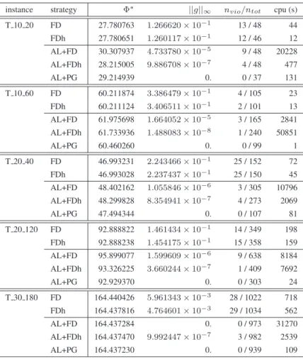
Table 1 displays the results for all the instances and for the analytical delay and load approxi-mations (by using Kleinrock’s function). For each instance, five strategies are compared. The first two strategies, “FD” and “FDh”, correspond to the flow deviation algorithm running on (QCRP) without the QoS constraints. “FDh” uses some path removal procedures as explained in [9]. The

(12)

last three strategies, “AL+FD”, “AL+FDh”, and “AL+PG”, consists in solving (QRCP) using the augmented Lagrangean method described in Section 2. The subproblem is solved by respec-tively the classical flow deviation, the flow deviation with path removal and the projected gradient method. For each strategy, the value of the optimal solution Φ∗ = Φ(x∗), the maximal violation ||g||∞of the solution over all the paths, the number nvioof active paths violating QoS constraints

over the active paths ntot, and the CPU time in seconds are reported. The maximal violation is

computed as follows: ||g||∞ = maxp∈Pk,k∈Kmax

©

0, g_pk(x∗)ª, where gk_p(x∗) denotes the QoS constraint on the path p for the demand k (cf. the constraints (4) in (QCRP)). In the objective function, the analytical approximation function fφs is kept in all cases for two reasons: first, this

evaluation function is not critical because it only gives a direction for the optimization, and also because it is a barrier function for the capacity on the arcs, which simplifies sub-problems.

instance strategy Φ∗ _||g||

∞ nvio/ntot cpu (s)

T 10 20 FD 27.780763 1.266620 × 10−1 _{13 / 48} ₄₄ FDh 27.780651 1.260117 × 10−1 _{12 / 46} ₁₂ AL+FD 30.307937 4.733780 × 10−5 _{9 / 48} ₂₀₂₂₈ AL+FDh 28.215005 9.886708 × 10−7 _{4 / 48} ₄₇₇ AL+PG 29.214939 0. 0 / 37 131 T 10 60 FD 60.211874 3.386479 × 10−1 _{4 / 105} ₂₃ FDh 60.211124 3.406511 × 10−1 _{2 / 101} ₁₃ AL+FD 61.975698 1.664052 × 10−5 _{3 / 165} ₂₈₄₁ AL+FDh 61.733936 1.488083 × 10−8 _{1 / 240} ₅₀₈₅₁ AL+PG 60.460260 0. 0 / 99 1 T 20 40 FD 46.993231 2.243466 × 10−1 _{25 / 152} ₇₂ FDh 46.993028 2.237437 × 10−1 _{25 / 150} ₄₅ AL+FD 48.402162 1.055846 × 10−6 _{3 / 305} ₁₀₇₉₆ AL+FDh 48.299828 8.354941 × 10−7 _{4 / 273} ₂₀₆₉ AL+PG 47.494344 0. 0 / 107 81 T 20 120 FD 92.888822 1.461434 × 10−1 _{14 / 349} ₁₉₈ FDh 92.888238 1.454175 × 10−1 _{15 / 358} ₁₅₉ AL+FD 95.899077 1.599609 × 10−6 _{9 / 638} ₈₁₈₄ AL+FDh 93.326225 3.660244 × 10−7 _{1 / 409} ₇₆₉₂ AL+PG 92.929370 0. 0 / 303 24 T 30 180 FD 164.440426 5.961343 × 10−3 _{28 / 1022} ₇₁₈ FDh 164.437816 4.764601 × 10−3 _{29 / 1034} ₅₆₂ AL+FD 164.437284 0. 0 / 973 31270 AL+FDh 164.437470 9.992447 × 10−7 _{3 / 982} ₂₅₃₉ AL+PG 164.437230 0. 0 / 939 109

Table 1: results for the analytical approximation.

As can be seen, taking the QoS into account (strategy AL) consumes a lot more time as it calls iteratively the FD algorithm. The difference can be really high, as for the instance T 10 60. However, the computed solutions using the AL strategy produce a very limited violation on the QoS, and for only few paths. In general, the number of paths carrying the traffic is higher since AL tries to use more paths to reduce the delay on each path. This has an impact on the value of the objective function. Values computed by FD and FDh are lower because QoS constraints are not taken into account. For the instance T 30 180, the FD strategy behaves rather poorly and stops too early. Thus, in that case, the AL strategy produces a better solution.

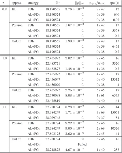
Table 2 displays a comparison between the analytical (KL) approximation and the neural network (NN) approximation (column “approx.”). For the neural network, two traffic scenarios (Poissonian sources and OnOff sources, which better approximate the nature of the traffic) are

(13)

considered. As the neural network consumes a lot of time, the experiments have only been done on a small instance (10 nodes, 22 edges and 40 commodities). In order to measure the impact of the global congestion, several throughputs (τ = 0.9, 1.0 and 1.1) have been tested. Each through-put τ is a common multiplying factor for all the demands. Thus, the bandwidth demands are both equally and globally increased. For each throughput and each approximation, three strategies haves been considered: the flow deviation with path reduction and without the QoS constraints (“FDh”), the augmented Lagrangean with either the FDh approach (“AL+FDh”) or the projected gradient (“AL+PG”).

τ approx. strategy Φ∗ _||g||_∞ _n

vio/ntot cpu (s)

0.9 KL FDh 18.190555 3.76 × 10−3 _{2 / 42} ₁₂ AL+FDh 18.190524 0. 0 / 39 640 AL+PG 18.190524 0. 0 / 38 0.02 Poisson FDh 18.190555 1.67 × 10−3 _{1 / 42} ₁₃ AL+FDh 18.190524 0. 0 / 39 5358 AL+PG 18.190524 0. 0 / 38 0.2 OnOff FDh 18.190555 1.90 × 10−3 _{2 / 42} ₁₃ AL+FDh 18.190524 0. 0 / 39 6461 AL+PG 18.190524 0. 0 / 38 0.2 1.0 KL FDh 22.455972 2.02 × 10−2 _{7 / 45} ₁₆ AL+FDh 22.483721 0. 0 / 43 3320 AL+PG 22.483877 1.48 × 10−7 _{1 / 36} _0.7 Poisson FDh 22.455972 1.04 × 10−2 _{4 / 45} ₁₇ AL+FDh 22.456047 0. 0 / 40 13312 AL+PG 22.456090 0. 0 / 38 4 OnOff FDh 22.455972 2.25 × 10−1 _{5 / 45} ₁₇ AL+FDh 22.730098 8.08 × 10−8 _{1 / 61} ₆₅₇₅ AL+PG 22.475819 0. 0 / 40 41 1.1 KL FDh 27.780724 8.28 × 10−2 _{8 / 46} ₁₄ AL+FDh 28.384249 1.71 × 10−5 _{3 / 69} ₁₅₀₅₁ AL+PG 28.029748 0. 0 / 37 84 Poisson FDh 27.780724 9.22 × 10−2 _{5 / 46} ₁₆ AL+FDh 28.384249 9.00 × 10−9 _{2 / 69} ₁₀₅₂₆ AL+PG 27.803175 2.62 × 10−6 _{2 / 45} ₄₁ OnOff FDh 27.780724 1.38 8 / 46 16 AL+FDh Failed AL+PG 28.218878 4.67 × 10−7 _{1 / 40} ₂₈₈

Table 2: results for both Kleinrock and NN approximations.

First, we can observe that the AL+FDh approach converges towards a feasible solution or a quasi-feasible solution. As the value ||g||∞remains small, output from the algorithm can be used

after a cleaning step. This holds for all values of τ . The FDh approach does not take the QoS constraints into account. Therefore, the QoS model cannot have any impact on the behavior of this method. This explains why, for any given value of τ , the optimal value of FDh remains the same whatever the approximation. For the same reason, the number of violated QoS constraints nvio

if higher than for AL. This number increases with higher congestion (higher throughput), along with the number of active paths (which is a classical result). About the AL approach, it can be noted that the impact of the delay model on the solution increases as the overall traffic load (i.e. the throughput τ ) increases. For moderate values of τ , AL gives solutions with fewer active paths. However this situation becomes different when the network comes close to saturation (to the QoS contraint point of view). At this point, it is difficult to keep a small number of active paths and the solution must use a lot more paths (i.e. τ = 1.0 with OnOff neural approximation of delay).

(14)

The last line of the table should indicate that the problem has become infeasible with respect to the OnOff QoS constraint. It still remains feasible with less accurate QoS approximations, namely Kleinrock and neural approximation with Poissonian traffic.

Overall, these experiments are useful in proving that the way QoS is approximated has a strong impact on the routing solution computed. According to the QoS approximation used, the routes that are obtained can differ significantly. It is worth mentioning that the higher the overall demand, the better balanced the load throughout the network. Moreover, the numerical results show that the neural network approach provides reliable estimates of the delay and it can be successfully applied on a simple context. It shows promises for QoS-based traffic control, routing and congestion avoidance in multiservice telecommunication networks.

Conclusion

The (QRCP) corresponds to the integration of QoS constraints, namely the end-to-end delay con-straints, into routing problems. Such constraints are hard to take into accound as they rely on path rather than on arcs. We have proposed an augmented Lagrangean method to solve the nonlinear problem. This approach involves the computation of an optimal solution to a routing problem with convex costs. Two algorithm have been proposed: a flow deviation approach and a projected gradient approach. The numerical results show that the later approach is a lot more efficient in many aspects (CPU time, quality of the solution, number of active paths in the solution). It allows telecom instances of realistic size to be solved in a reasonnable amount of time. Two functions have been tested to model the delay: the analytical M/M/1 approximation and a neural network. The neural network provides a better approximation as it is able to take the differenciation of ser-vice (DiffServ) into account. It has been trained on two traffic scenarios (Poisson and OnOff). The numerical results show that the overhead when using a neural network instead of an analytical function can be significant. The solutions produced can also differ significantly since the neural network provides a more realistic approximation.

As the augmented Lagrangean method cannot guaranty the optimality of the solution, an exact method still remain to be developped, even if the gaps produced here are small. Another approach could be to embed the augmented Lagrangean into a multistart procedure to try to reach the optimal solution. Other lines of work would be to deal with the minimization of the maximal congestion and consider end-to-end delay and loss rate constraints.

References

[1] Ben-Ameur, W., and Ouorou, A., “Mathematical models of the delay constrained routing problem”, Algorithmic Operations Research, 1(2), 2006.

[2] Bertsekas, D., “On the Goldstein-Levitin-Polyak gradient projection method”, IEEE Trans-actions on Automatic Control, AC-21(2), pp. 164–174, 1976.

[3] Bertsekas, D., “Constrained Optimization and Lagrange Multiplier Methods”, Academic Press, 1982.

[4] Bertsekas, D., and Gafni, E., “Projected Newton methods and optimization of multicommod-ity flows”, IEEE Transactions on Automatic Control, AC-28(12), pp. 1090–1096, 1983.

(15)

[6] Bertsekas, D., Nonlinear Programming, second edition, Athena Scientific, 1999.

[7] Bienstock, D., and Raskina, O., “Asymptotic analysis of the flow deviation method for the maximum concurrent flow problem”, Mathematical Programming, 91(3), pp. 479–492, 2002.

[8] Conn, A.R., and Gould, N., and Sartenaer, A., and Toint, P.L., “Convergence properties of an augmented Lagrangian algorithm for optimization with a combination of general equality and linear constraints”, SIAM J. on Optimization, 6(3), pp. 674–703, 1996.

[9] Duhamel, C., and Mahey, P., “Multicommodity flow problems with a bounded number of paths: A flow deviation approach”, Networks, 49(1), pp. 80–89, 2007.

[10] Fratta, L., Gerla, M., and Kleinrock, L., “The flow deviation method: An approach to store-and-forward communication network design”, Networks, 3, pp. 97–133, 1973.

[11] Giordano, S., Potts, M., Smirnov, M., and Ventre, G., “Advances in QoS”, IEEE Communi-cations Magazine, 41(1), pp. 28–29, 2003.

[12] Mahul, A., and Aussem, A., “Learning with monotonicity requirements for optimal routing with end-to-end quality of service constraints”, in Proceedings of the 14th European Sympo-sium on Artificial Neural Networks (ESANN’2006), pp. 455-460, Bruges, Belgium, 2006.

[13] Mykoniati, E., and al., “Admission control for providing QoS in DiffServ IP networks: the TEQUILA approach”, IEEE Communications Magazine, 41(1), pp. 38–44, 2003.

[14] Ouorou, A., Mahey, P., and Vial, J.-P., “A survey of algorithms for convex multicommodity flow problems”, Management Science, 47(1), pp. 126–147, 2000.

[15] Wang, Z., “On the complexity of quality of service routing”, Information Processing Letters, 69, pp. 111–114, 1999.