How Selection Techniques on Traffic Data Sets Can Help in Estimating Network Vehicle Emissions

HAL Id: hal-01930242

https://hal.archives-ouvertes.fr/hal-01930242

HAL is a multi-disciplinary open access archive for the deposit and dissemination of sci-entific research documents, whether they are pub-lished or not. The documents may come from teaching and research institutions in France or abroad, or from public or private research centers.

L’archive ouverte pluridisciplinaire HAL, est destinée au dépôt et à la diffusion de documents scientifiques de niveau recherche, publiés ou non, émanant des établissements d’enseignement et de recherche français ou étrangers, des laboratoires publics ou privés.

in Estimating Network Vehicle Emissions

Nicole Schiper, Delphine Lejri, Ludovic Leclercq

To cite this version:

Nicole Schiper, Delphine Lejri, Ludovic Leclercq. How Selection Techniques on Traffic Data Sets Can Help in Estimating Network Vehicle Emissions. Journal of Earth Sciences and Geotechnical Engineering, Scienpress LTD, 2016, 6 (4), pp.51-69. �hal-01930242�

Scienpress Ltd, 2016

How Selection Techniques on Traffic Data Sets Can

Help in Estimating Network Vehicle Emissions

Nicole Schiper1, Delphine Lejri1 and Ludovic Leclercq1

Abstract

Road traffic is a major source of air pollution in urban areas. Policy makers are pushing for different solutions including new traffic management strategies that can directly lower pollutants emissions. To assess the performances of such strategies, the calculation of pollution emission should take into account traffic dynamics.

The use of traditional on-road sensors (e.g. inductive loops) for collecting real-time data is necessary but not sufficient because of their expensive cost of implementation. It is also a disadvantage that such technologies, for practical reasons, only provide local information. Some methods should then be applied to expand this local information to large spatial extent. These methods currently suffer from the following limitations: (i) the relationship between missing data mechanisms/patterns and the estimation accuracy, both cannot be easily determined and (ii) the calculations on large area is computationally expensive. Given a dynamic traffic simulation, we take a novel approach to this problem by applying selection techniques that can identify the most relevant locations to estimate the network vehicle emissions. This paper explores the use of a statistical method, i.e. the Lasso regularized generalized linear models, as powerful tool for selecting the most relevant traffic information on a network to determine the total pollution emission.

Keywords: Vehicle emissions, Traffic data selection, Inductive loops,

Spatial-temporal correlation, Lasso

1 Introduction

According to the European Union (European Commission, 2015), road traffic accounted for 65% of Carbon Monoxide (CO), 41% of hydrocarbons (HC), 48% of Nitrogen Oxides (NOx) and 30% carbon dioxide (CO2) released into the atmosphere. Reducing emissions can be achieved either by improving vehicle technologies or by implementing measures to modify the pattern of car use: reduction of car use, diminution of events that produce high emissions rates (i.e. congested periods). The impact of transport control measures on emissions is typically measured in terms of reduction of vehicle emissions brought about by these strategies. Currently, many of the transport models incorporate technologies to measure pollutants from road traffic, in order to assist in the evaluation of transport strategies taking into account their respective environmental impacts. Most of these proposals is associated with new technologies for vehicles and fuels. This type of measurement, however, presents results only in a long term. To ensure a future decrease in transport-related CO2 emissions, it is essential that most of users exploit cleaner vehicles, use low-Sulphur and unleaded fuels, and increase the turn-over rate of their ageing vehicle fleet. This type of strategies need years to be implemented and to get the first results of pollutants reduction. However, measures related to planning traffic influence on vehicle operating characteristics have a good result in a short-term (Franceschetti et al, 2013). The extent of the results of the implementation of planning measures traffic and cost/benefit, however, cannot be evaluated without the use of quantitative models for pollutants estimate from road traffic, or simply, emission models (De Vlieger, 2000).

In general, the emission models perform quantification of contaminants in two stages. The first consists in determining a set of emission factors that specify the rate at which the emissions are generated. The second step involves estimating the activities of vehicles. The emission inventory is calculated by multiplying the results of these two steps. The emission models need, therefore, data on the activity and behavior of the traffic. It is commonly used for this purpose, driving cycles developed to represent the operation of a vehicle in a manner similar to the real world (Ahn and Rakha, 2008). However, sometimes these cycles can represent traffic behavior of a refined form (Al Barakeh, 2012). Currently we observe the great use of emission models that aggregates the traffic models. The direct use of traffic models for the calculation of vehicle emissions becomes interesting as it provides a refined description of traffic conditions both in space and time. Furthermore, there are able to predict the impacts of new traffic management strategies or new road layouts.

Good understanding of traffic dynamics is fundamental to assist in choosing the most effective study strategy to be adopted for each type of problem being treated. This work allows taking into account more precisely, the effects of traffic dynamics on network and for that precision, a significantly increase of volume processed data and time calculation to get some results. This complexity is

necessary when it comes to describe a fine resolution of space and time the evolution of emissions. It may seem excessive, but when it is fair to compare different projects in relation to their global impacts.

The aim of the paper is to work on the sampling of traffic and emissions data to reduce significantly the volume of data to be processed while keeping an accurate estimate of the overall results in terms of air pollution. It is thus to define the minimum sample in time and in space as a function of the emission model. For example, rather than making calculations on each part of the network, a set of links and reference time periods will be identified to perform the calculations. Note that spatial-temporal correlations happen because of congestion waves and changes in demand that propagate through the network. Thus it is important to define a methodology able to take into account the correlations for the segmentation of the population to define a representative sample. Moreover, the dynamic traffic and the traffic conditions changes on different time horizons (from the second to the day). It is important to correctly estimate the emissions but also their temporal estimation to consider the time factor. This may lead to a particular sampling differentiated according to the periods of the day. For this, a good understanding of the coupling between traffic models and emission models will be profitable.

2 Objectives and Methodology

Traffic data sampling comes to identify effective methods of sampling in order to determine with a sufficient degree of accuracy the characteristics of pollutant emissions in the total population (average, total…). We explore the use of a statistical method, i.e. the Lasso regularized generalized linear models (Friedman et al, 2010), as powerful tool for selecting the most relevant traffic information on a network to determine the total pollution emissions. A neighborhood of Paris, part of the 6th district, was used as the basis for our study. The network was built as part of the project ISpace & Time (2013) funded by the ANR (the french national research agency). The network is composed of 234 links, 93 crossroads, 19 entries, 21 exits including 4 parking’s inside and 27 traffic lights. All links have directions, bus lane, traffic lights times and allowed turning movements inside crossroads. This network was implemented in the microscopic traffic simulator called Symuvia developed by the laboratory LICIT (Laboratoire Ingénierie Circulation Transport). This traffic simulator is used to define the traffic settings which represents, in the most realistic way, the traffic conditions on the neighborhood. There are three main settings that should be taken into account: temporal evolution of demand, origin-destination matrix and assignment matrix. In order to avoid long calculation time to simulate 24 hours of traffic, the 6 most relevant hours for typical daily traffic are considered. The temporal evolution of the demand is represented by two peak hour’s traffic: morning and evening. The

first one corresponds to the intense demand distributed in short period of time while the evening peak have a moderate demand distributed in a longer time. In order to simulate the traffic in the proposed network, only passenger cars were modeled. On each link are placed the two types of sensors. The 6 hours of simulation will be divided in 24 periods of 15 minutes, and for each one the traffic information will be recovered in every link of the network. Two types of virtual sensors are used during the simulation. MFD loops provide a complete information of the local traffic as: total travel time, travelled distances by cars and their mean speeds. Inductive loops just give the number of vehicles and the mean speed observed in the middle of each link. This loop type is an example of traffic data used by policymakers to evaluate their strategies to regulate the networks. It is important to note that the spatial traffic information at link level only come from MFD sensors. This can only be derived by simulation. A sensibility analysis between both to quantify emissions will be discussed in the next section.

In order to be statistically representative, a great number of observations (i.e. simulations) and various traffic states in space and time are needed. To this end, the number of simulations has been set at 400. The difference between them will be the randomly demand for each entry and period of time.

In order to assess traffic emissions, the main purpose of emission models consists in estimating emission data on different spatial and temporal scale. They range from calculations at a microscopic scale (i.e. for a single vehicle or for a street) to a macroscopic calculation (i.e. regional, national and global levels) through the inventory of an urban transport network. Furthermore, the models differ by the way they take into account the following parameters: pollutants “covered”; type of emissions; fleet composition (vehicles categories and age); driving patterns (average speed only or instantaneous speed and acceleration). About the last, the spatial mean speeds used in the emission calculations are calculated as the ratio of the total travelled distance and the total time spent by vehicles for every link and time period. For our study will be used COPERT IV emission model to estimate the pollutants from the variables described above.

This paper is organized as follow: First will be presented how different source of traffic information can affect emissions; The second part presents the sampling method used to select the most relevant traffic and the datasets used; Finally, the results will be discussed.

3 Influence of Variable Definition on Emissions

In order to calculate emissions using COPERT IV, two traffic information are required: travelled distance and mean speed. Using the inductive loops as traffic information source, travelled distances need to be calculated from the vehicle flows. To this end, two link length definitions will be used. The two definitions for link lengths are static and dynamic one: The first called static length, considers the geometric link length, so the length between its begin and end including the

distance between the exit of link and barycenter from the upstream crossroad, if it exits. The second length called dynamic, takes into account the extra distances of allowed movements inside of the crossroads. The latter allows to know the real distance travelled by vehicles on the link and inside of the crossroad, according to flow, instead of estimated them using geometric measures. It is interesting to understand that the geometric link length is a static magnitude and does not depend to traffic flow. Unlike that, the dynamic link length depends completely of the traffic flow on each link and crossroad, hence the name dynamic.

As described above, the traffic data will be used as input in emission models to calculate pollutant emissions. Two pollutants will be considered, the CO2 (carbon dioxide) that have most impact in greenhouse effect and the NOx (nitrogen oxides) which impact the public health. The emission assessment is done according to the choice of parameter settings such as fleet composition, type of emissions and speed-dependent emissions. The 2015 French fleet composition was chosen and the study will concentrate on hot emissions. To calculate the amount of each pollutant, the speed-dependent curves will be used. The latter provide emission factors for each average speed bigger than 10 km/h. Considering that, for average speeds less than 10 km/h, the emissions will be calculated using the emission factor equal to 10 km/h. The equation that will be used to quantify emissions with the speed curve is shown below:

Definition 3.1

Calculation procedure.

𝑬(𝒕) = 𝑷(𝒕). 𝑬𝑭(𝑺)

Where:

E(t): Total emission for each traffic time period (g/km) P(t): Total travelled distance on traffic link (km)

EF(S): Emission facto for average speed S and for pollutant S: Average vehicles speed on traffic link (km/h)

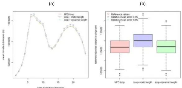
As said before, the travelled distance that comes from the named MFD loops is used as reference to evaluate the calculation methods of the total traveled distance using traffic data from inductive loops. To obtain the total traveled distance to use as input on the emission model, two hypotheses are explored using both link lengths. Figure 1 shows the comparison of these two hypothesis with the reference.

Both figures make comparison of network travel productions. Network travelled distances is defined by the total travelled distance considering the entire network. “MFD loop” is the reference values, “Loop + static length” corresponds to total travelled distances considering the geometric link length and finally the “Loop + dynamic length” are the values considering the dynamic length. The last one is the method that better corresponds with the reference values with only 1% of average error (over 400 simulated values). Note that travelled distances calculated using geometric length have almost the same distribution than the travelled distances

calculated using the dynamic link length. In fact, this last is not surprising because the total travelled distances are the product between the number of vehicles that pass at the sensor in a given link and the mean travelled distance of the same link.

Figure 1: Network travelled distance comparison.

Considering that, we assume that all vehicles passed through the sensor did the same travelled distance. Consequently, this travelled distance will be a bit overestimated, at about 3% as shown in Figure 1(b), because it considers that all vehicles passed in front of sensor run through the totality of geometric link length and sometimes it is not the case. The differences between them are small considering they were calculated at network level (i.e. time and space gathered). This difference also can be seen in figure 1(b) that shows distribution values of each one and the relative mean error of each method in comparison to the reference values. Within a perspective of policymakers and considering the low errors of travelled distances (under 3,5% in average over 400 simulations) the method using geometric length allows, in an easy way, to determine the travelled distance of a link or network directly using the data collected by a sensor and geo-referenced maps without having to use simulations to this purpose.

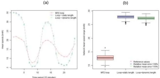
The second traffic variable that need to be analyzed to estimate emissions is the mean speed. The network under study represents an urban area which has low mean speed over 15 minutes and its variation is between 1 km/h and 50 km/h locally. The mean speeds from inductive loops are both overestimated and reached great relative mean errors, at about 115% in average error, as shown in figure 2. The range of mean speeds at network scale are very different when MFD and inductive loops are compared. The range of mean speeds values vary between 5 and less than 35 km/h. These low speeds are totally normal when an urban area is represented. Furthermore, these low speeds have an importance when the emissions are calculated, because they have higher emission factors. The great differences between the mean speed from MFD and Inductive loops are more

evident in the periods of free-flow (traffic lights influence), and can reach 14km/h of difference between both, than the periods which the network is considered congested, so this difference vary according to the traffic state. This fact is explained in how the mean speed is considered at link level. For inductive loops, the mean speed considered to all link length is measured from a point in the middle of each lane. As most of links have small length, so the vehicles run through the sensor are still accelerating. Unlike the inductive loops, the MFD sensors calculate the mean speed considering the full-length of each link (spatial approach) and not a point and it is possible only through simulations. These considerations explain the differences between mean speeds from the sensors. The spatial mean speed needs the simulation environment to determine it precisely.

Figure 2: Network mean speeds comparison.

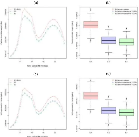
The network pollutants were calculated using the total travelled distance and mean speed recovered by sensors for each 15 minutes’ time range. Then, it was made the sum of emissions for all links and period of time per daily traffic (i.e. simulations). This method was used to get the emissions from MFD and inductive loops and all previously described calculation methods. For all studies about emissions, the MFD results from local calculation were our reference values, because they used a finest description of traffic and represent the exact values on each simulation.

The figure 3 compares the pollutant emissions from both sensors: (a) and (b) correspond to carbon dioxide network emissions; and (c) and (d) for NOx network emissions. As can be seen, the pollutant emissions calculated using local traffic data from inductive loops show lower values than from MFD sensors. These lower amounts of emissions are due to the fact that inductive loops consider much higher speeds than MFD sensor and consequently lower emission factors; these differences are most evident in congested state. As shown in figure 2 the network mean speeds from inductive loops are between 5km/h and 35km/h instead of

7km/h and 25km/h from MFD loops, consequently high speed values tend to have lower coefficient of emissions.

The pollutant emission is the product of traveled distance and the corresponding emission factor for given pollutant determined by mean speed. The difference between the three travelled distances are very small (figure 1) but the mean speed comparison shows different speeds from both sensors and that ending to underestimate around 14% the network emissions using the traffic data from this loop ((b) and (d) in figure 3).

Figure 3: Network pollutant emission comparison: (a) and (b) corresponds to CO2

network emissions; and (c) and (d) corresponds to NOx network emissions.

Two sources of information were analyzed: MFD and inductive loops. Traffic data from inductive loops tends to be overestimated in comparison to MFD values. Travelled distance has a little average increase of 2% in average while mean speed can reach over 100% of disparity. These gaps lead to an underestimation of emissions around 14% at network level. For free-flow periods this disparity is at

(a) (b)

about 1% compared to congested periods that can reach 14% of difference.

To assess the emissions accurately and to obtain a selection using the accurate values, after having compared all variables and how they affect the emissions, the traffic data from MFD loops will be used to apply the selection methods.

4 Methodology

4.1 The Sampling Method

The least absolute shrinkage and selection operator (LASSO) (Tibshirani,1997) is a modern statistical method that has gained much attention over the last decade as researchers in many fields are able to measure far more variables than ever before. Linear regression suffers in two important ways as the number of predictors becomes large: First, over fitting may occur, meaning that the fitted model does not reliably generalize beyond the particular data observed; second, it becomes difficult to interpret the fitted models. The Lasso addresses both of these issues by identifying a small number of predictors on which a reliable model can be built.

4.2 The Data Sets

Two types of datasets were built to help characterizing the dynamic behavior of network. They were built for each variable as total travelled distance, mean speed, CO2 and NOx emissions. The datasets structures are explained below.

The first dataset called static considers only the daily traffic values for each link on the network. The purpose is to estimate variables values at network level considering daily traffic values for travel production, mean speed and emissions. All links have their periods of time gathered, giving the total or mean values for each one. For example, considering the travelled distance variable, each link has the total traveled distance for daily traffic, which means the values for each link are the sum of travelled distances of all time periods. To illustrate, the regressors are the links and their observations are the total traveled distance with all periods gathered for each simulation. In the same way this dataset was built for CO2 and NOx emissions, they are represented as sum of total emissions in periods of time. In contrast to, the average speed on links are calculate in function of their means speeds and travel times. The values represent the average mean speeds over periods of time and are calculate for each link separately.

The second dataset that will be studied is called dynamic and considers the traffic data for each 15 minute' periods on each link. But its structure was built to have as regressors: links and their periods of time. The selection methods will be applied both on link and time period. The idea is to identify for each link which time periods are really relevant. The observations are their respective values for each simulation. This dataset allows to estimate the network daily values using 15 minute' period traffic data.

Both datasets provide as results network values, that means the variables values considering the entire network for a daily traffic. The results from the selection method and a comparison between them will be study in the next section.

5 Results

The variables are structured as 𝑛 × 𝑝 matrix, which 𝑝 are the links represented in the network while 𝑛 are the observations values for each link. Each link has 400 observations and they were split up randomly in two parts: the first represents 2/3 of the matrix and was used as training set where LASSO was applied and settled a model; and the second part, 1/3 of original matrix, represents the validation set where the LASSO settled model defined in training set will be validated and the errors associated will be quantified.

5.1 Static Data Sets

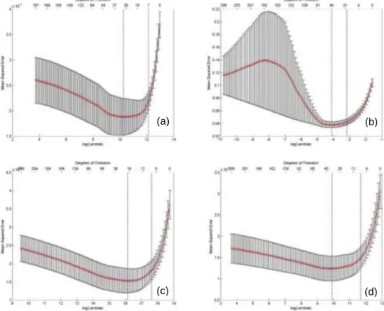
Figure 4: The ʎ cross-validate for each variable in static data sets: (a) represents travel production; (b) is the mean speed; (c) is the CO2 emissions; and (d) corresponds to NOx

emissions. The model retained for each variable corresponds to the rightest vertical line.

The model proposed by 𝜆 with one standard-error from the minimum square error was the model retained for all variables because it selects less predictors with the same error level compared to 𝜆 model (Tibshirani,1997). The results are presented only for this model. In figure 4 are shown the 𝜆 cross-validated for each variable in static dataset. It represents the estimated prediction error curves

(a) (b)

and their standard errors for the variables in static datasets: (a) is the model settled for travelled distance, (b) for mean speed, (c) for CO2 and (d) for NOx emissions. Each curve is plotted as a function of the corresponding complexity parameter 𝜆. The horizontal axis has been chosen so that the model complexity increases as we move from right to left. The estimates of prediction error and their standard errors were obtained by tenfold cross-validation. The least complex model within one standard error of the best is chosen, indicated by the vertical lines. The left vertical line is the model with minimum error and the right one is the model settled using the one standard error rule (the model that will be studied). The top of each plot is annotated with the size of models.

The LASSO made a selection over 230 links of the network and gives us models with: 7 links for travelled distance which the model that can explain the data in 43% considering the confidence interval of 95%; selected 19 links for mean speed with 64% of data explained by the model; and 11 links for both pollutants emissions with model that explain 54% of data in CO2 emissions and 55% of data explanation in NOx emissions.

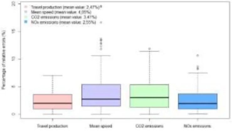
The relatives’ errors were calculated comparing the results (values predicted by the model established) with the reference values (Y). The figure 5 shows the distribution of associated errors in each variable for the static dataset.

Figure 5: Percentage of error between the resulting variable values of the model with selected links and the original values of variables (Y).

All variables have small average error considering models that have less than 10% of the links of the network selected. More than 50% of the data has errors less than 5% considering average errors between 2,50% and 4%. A cross-analysis was made to observe if one of the 4 models could be used to determine other variables values with the goal to have a set of selected links that can be used to quantify network values for all variables.

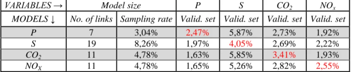
The table 1 shows the average percentage of error of the selected links model established by the variables in the lines applied on the variables disposed in the columns. It also shows the average error on validation set of the selected links from one variable applied to another one and the average error for the Lasso

applied on the variables. The aim here is to investigate the possibility of using a set of selected links to determine all other variables.

To this end, in the same training set, a linear regression was performed on the links selected by Lasso. The objective is to find the beta values of each selected link adapted to the variable under study. In general, for all cases, the average errors values remain in the same range as the Lasso method. The links selected in common for the 4 variables were also compared and the ratio is presented in the table 2 to complete the analysis.

Table 1: The average error of the model established with one variable applied to another. The red values represent the lasso result errors by variable.

VARIABLES → Model size P S CO2 NOx

MODELS ↓ No. of links Sampling rate Valid. set Valid. set Valid. set Valid. set

P 7 3,04% 2,47% 5,87% 2,73% 1,92%

S 19 8,26% 1,97% 4,05% 2,69% 2,22%

CO2 11 4,78% 1,63% 5,85% 3,41% 1,93%

NOX 11 4,78% 1,65% 5,26% 2,82% 2,55%

It is possible to observe in table 2 that travelled distance and spatial mean speed variables have no common selected links. That can be explained by their opposite behavior: the travelled distance is a linear variable over the links whereas the spatial mean speed is not. In the light of these considerations, two conclusions can be observed: (i) the strong correlation between travelled distance and spatial mean speed allows to determine each emissions from their sampling, because they are dependent from these both traffic variables; and (ii) the fact that both can be used to determine other variable values using a simple linear regression, leads us to conclude that it does not exist just only one acceptable sampling (set of links). Thus there is ample evidence of the selection flexibility. The model with less selected links will be the best choice, especially in practical point of view, for transportation managers when they decide to outfit links on the network. All models defined by Lasso or by linear regression were validated on a validation set completely different from the training set used to apply them. Yet, to be able to compare the results, the training data and the validation data were the same throughout this study.

Table 2: Ratio of common selected links between variables.

MODELS ↓ P S CO2 NOX

P 100% 0% 57,1% 42,8%

S 0% 100% 0% 0%

CO2 36,4% 0% 100% 72,7%

The average errors remain in the same range with the four links sets: 2% for NOx emissions and travelled distance and 3% for CO2 emissions. So, various sampled links could provide an estimation of traffic and emission variables over the network with reasonable error.

Considering the low sampling rate in each variable, and also their low average errors and taking into account that they have some common selected links, it also was considered to study the possibility to make the union or/and the intersection between the traffic variables and between the emissions pollutants. For example, the selected links identified by the shrinkage method for the traffic data, total travelled distance and spatial mean speed, will be put together (union of selected links between two variables) to apply a linear regression and obtain a new model with adjusted beta values for each predictor (links). In the same way, the union between CO2 and NOx was considered. Taking into account that some variables have common links, it was considered the intersection between them. The advantage of the intersection between them is the possibility to have a model with less predictors than the model established by the union of them. The associated errors were quantified for each resulting variable values. The average error of each linear regression is shown in table 3 and was calculated for each variable considering each situation (union or intersection).

Table 3: The average percentage of error from the linear regression model settled on the union or intersection between variables of the same nature.

VARIABLES → Model size P S CO2 NOx

MODELS ↓ No. of links Sampling rate Valid. set Valid. set Valid. set Valid. set

P U S 26 11,30% 1,78% 3,48% 2,55% 2,18%

P ∩ S - - - -

CO2 U NOX 14 6,09% 1,62% 5,25% 2,80% 2,12%

CO2 ∩ NOX 8 3,48% 1,68% 6,61% 2,98% 2,10%

The selected links in total travelled and spatial mean speed are completely different, so they have no common links. The union of traffic variables allows estimating all variables values with the same accuracy as the Lasso selection applied in each one separately. The distribution of error values varies from 0,1% to less than 7% considering 95% of confidence interval in general for all variables. When selection in travelled distance showed in table 1 is compared with the union between the traffic variables and also with the union of the pollutants emissions, it is possible to observe that the distribution of errors is less dispersed with the union of selected links. In contrast to, the union models have more links than the model established by travelled distance in table 1, which explains the fact that the errors are less dispersed. When the same comparison is made with the intersection between the selected links of the pollutants, they have almost the same amount of selected links and average error values. If we compare the models of the pollutants in table 1 with the intersection between them, it is interesting to observe that even

if it reduces the selection’s size (in this case the selection passes from 11 to 8), the results remain the same. So, the union of selected links identified by the shrinkage method for the two variables that characterize daily values of the traffic and the linear regression model established with these ones, can estimate the network daily values with a low average error and using just 11% of the network links. When it comes to the emissions, the best choice is the intersection between them. Considering only 8 links (3,5% of the network), all the variables can be estimate with acceptable error, around 2% for travelled distance, 3% for pollutants emissions and less than 7% for spatial mean speed.

The shrinkage method called Lasso was used as linear regression selection method to perform a selection of the most relevant links on the network for traffic and emissions variables. For each one, a model was established with a set of links and the weights of each one. Using total/mean daily information as input is enough to estimate with accurateness the variables. The analysis concludes that the links selected on the travelled distance presents better results in terms of minimum number of links necessary to estimate with accuracy traffic and emissions daily values. To sum up, we can deduce that a finest traffic data is not necessary to quantify and determined daily traffic and emissions at network level, the daily values are enough information to obtained it.

5.2 Dynamic Data Sets

(a) (b)

Figure 6: Estimated prediction error curves and their standard errors for the variables in dynamic/dynamic datasets. Each plot represents: (a) travelled distances, (b) spatial mean

speed, (c) CO2 and (d) NOx emissions.

As explained before the model proposed by 𝜆 with one standard-error from the minimum square error was the model retained for all variables. In figure 6 are shown the 𝜆 cross-validated for each variable.

In travelled distance, the 30 predictors selected represents 25 links on the network. 14 predictors correspond to morning traffic against 16 in the evening (the morning traffic are represented by periods of time from 1 to 12 and the evening from 13 to 24). It is interesting to observe that the selected periods of time represent the free-flow periods. These datasets provide as result the daily values of the network as static datasets. The models established for travelled distance can explain the data at 52% (which refers to 95% of confidence interval) and give us the results with a mean error equal to 3,6%. If we compare the travelled distance selection between static and dynamic datasets, we have 6 common links, which means that 6/7 selected links on travelled distance with static dataset are included in the model established with the dynamic dataset. The spatial mean speed had 20 periods of time selected, which represents 18 links. In the 20 predictors, 12 are from morning peak and 8 are from the evening. The model can explain 56% of the data with average error of 5,11%. All periods selected represents a free-flow state in the network. This dataset gives us as result the average daily speed in the network. If we compare with the selection made in static dataset, they only have 6 links in common.

The figure 6(c) represents the selection made in CO2 emissions: 12 predictors are selected. They represent 11 links on the network. 5 among the selected time periods are in the morning assignment, respectively 7 in the evening assignment. 8 predictors among 12 are the same (link and period of time) between CO2 and travelled distance. Any predictors selected in mean speed were selected in CO2. The periods selected represent also a free-flow state on the network. The model built by LASSO can explain 56% of the data with average error at about 3,6% as show in figure 6. The figure 6(d) represents the selection made in the NOx emissions. This variable has 29 predictors selected and they are represented by 23 links with 6 predictors that represent morning assignment and 23 predictors for evening assignment. This variable selected more evening time periods than the other variables in this dataset. The model built by Lasso using the selected links and time periods can explain 64% of data with average error of 2,8%.

Figure 7: Percentage of error between the resulting variable values of the model with selected links and time periods and the original values of variables (Y).

Analyzing the results of all variables, in most of them, the free-flow time periods are selected, which means states that the network is charged by vehicles but traffic flows normally. The number of selected time periods are equilibrated between morning and evening assignment with exception the NOx that have more selected periods in the evening. The emissions models provide selected links and time periods completely different in comparison to the selection obtained with mean speed. The daily values of each variable were calculated using the validation set and their relative errors were calculated. The average errors are almost the same as the other dataset. 75% of the data have an error lower than 7%. In figure 7, the percentage of error in the validation set are shown, when network variables were calculated using the model with selected predictors.

As in static dataset, a cross-analysis was conducted to observe if one of the 4 models could be used to determine other variables’ values and their comparison are presented in table 4.

As noted in the table 4, the same considerations made for static dataset are applied here. It is possible to use selected links of one variable to determine the other ones with the same accuracy as Lasso did. The predictors selected for all variables were analyzed. Unlike the spatial mean speed, the other three variables have predictors (link and time period) in common and they are shown in table 5. The most important conclusion is that the model defined in CO2 emissions has 75% of same selected links and time periods, which means a strong dependence of the CO2 with travelled distance for time period.

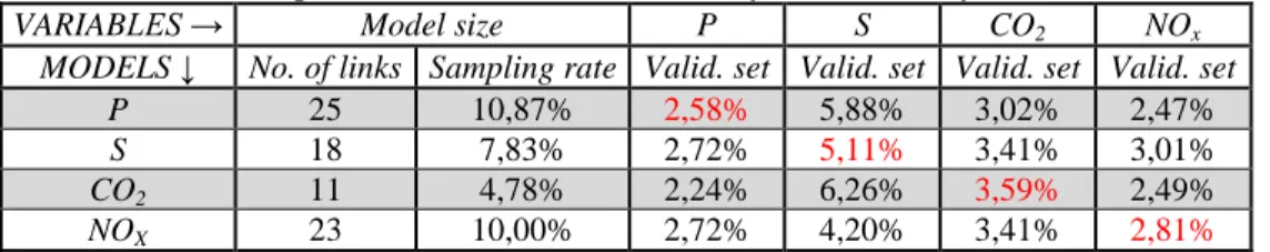
Table 4: The average error of the model established with one variable applied to another. The red values represent the lasso result errors by variable in dynamic data sets.

VARIABLES → Model size P S CO2 NOx

MODELS ↓ No. of links Sampling rate Valid. set Valid. set Valid. set Valid. set

P 25 10,87% 2,58% 5,88% 3,02% 2,47%

S 18 7,83% 2,72% 5,11% 3,41% 3,01%

CO2 11 4,78% 2,24% 6,26% 3,59% 2,49%

A second study was conducted to observe if a linear regression model including a set of selected predictors could be used to determine all variables values as studied in the previous dataset and the results are presented in table 6. All linear regression models applied on all variables have low average percentage of errors in the validation set.

Table 5: The common selected links and time periods between variables.

MODELS ↓ P S CO2 NOX

P 100% 0% 30,0% 26,7%

S 0% 0% 0% 0%

CO2 75,0% 0% 100% 33,3%

NOX 27,6% 0% 13,8% 100%

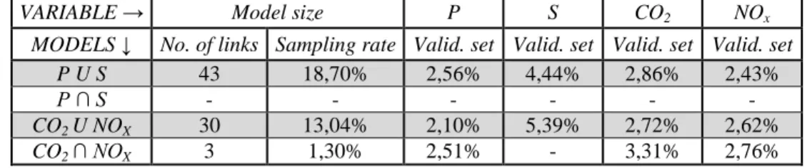
The union between the traffic variables has a model size equal to 50 predictors that corresponds to 43 links of the network with all of periods with free-flow state. The union between the two pollutants emissions is composed of 37 selected predictors over the 5520 of the original matrix. Its model corresponds to 30 selected links with also most of periods in free-flow state. The last linear regression model, the intersection between CO2 and NOx, has only 4 predictors that represent 3 links of the network with all periods in free-flow. The last model can accurately assess, with 15 minutes’ traffic data on only 3 links identified by Lasso, the daily values of the network for travelled distance and pollutants emissions considering that the data are explained in, at about 60%, considering the confidence interval of 95%. The linear regression on the selected links intersection does not have statistical representativeness for the network spatial mean speed. In practice, this type of results needs a finest traffic data over a year and a pre-processing data to obtain local emission and finally a model that can estimate 3 of 4 variables with reasonable error.

Table 6: The average percentage of error from the linear regression model settled on the union or intersection between variables of the same nature.

VARIABLE → Model size P S CO2 NOx

MODELS ↓ No. of links Sampling rate Valid. set Valid. set Valid. set Valid. set

P U S 43 18,70% 2,56% 4,44% 2,86% 2,43%

P ∩ S - - - -

CO2 U NOX 30 13,04% 2,10% 5,39% 2,72% 2,62%

CO2 ∩ NOX 3 1,30% 2,51% - 3,31% 2,76%

6 Conclusion and Discussion

In this paper we first show that Inductive loops tend to underestimate emissions in comparison to MFD loops. Second, based on Lasso selection method, we construct a model that can estimate emissions from a small group of predictors

(links or links with their periods of time) based on observations values. Four variables were studied: travelled distance, mean speed, CO2 and NOx emissions. The difference between static and dynamic dataset are: (i) the static one has as predictors the links of the network and as observations the daily values of each link according to the variables under study; (ii) the dynamic dataset has as predictors the periods of time of each link and as observations the 15 minutes’ variable values that respectively correspond to the link and period of time. Both matrices are compared with a vector that represents the network daily values for each simulation. The idea of the first dataset is to identify the most relevant links in the network using daily values. With the second dataset, we identify in each link which time periods are really relevant. This method can help to identify where it is possible to place, in reality, on-road sensors to estimate network variables. This first analysis shows that selection on daily travelled distance is the best model that can estimate the spatial mean speed and both pollutants emissions. The last selected only 3% of the network’ links with an average error less than 6%. In order to qualify the effectiveness of Lasso method for environmental assessment, these results have to be confirmed with other data sets and compared to other selection methods. However, the daily emission value is often not sufficient if we are interested in population exposure to pollutants. Thus, further analysis will first be conducted in order to find the best link selection to assess 15 min ‘s emissions.

The applications of such techniques are numerous. In addition to significant improvement in computing time, the development of appropriate sampling methods could also help to identify key areas of a network or travel types and thus, help to improve the assessments a posteriori (optimal positioning stations measurement, definition references tours for vehicles with embedded measurement means, ...). The technique covered by this work could also be useful in real-time assessments of quantify emissions. Indeed, sensor networks for air pollution are generally sparse and does not discriminate specifically the contribution of road traffic.

References

[1] A. Kyoungho and H. Rakha, The Effects of Route Choice Decisions on Vehicle Energy Consumption and Emissions, Transportation Research Part

D: Transport and Environment, 13(3), (2008), 151 - 167.

[2] Z. Al Barakeh, Suivi de Pollution Atmosphérique Par Système

Multi-Capteurs–méthode Mixte de Classification et de Détermination D’un Indice de Pollution, EMSE, Saint-Etienne, 2012.

[3] T.V. da Rocha, Quantification Des Erreurs Associées à L’usage de

Consommation En Carburant, École Nationale des Travaux Publics de l’État,

Lyon, 2013.

[4] I. De Vlieger, D. De Keukeleere and J. G. Kretzschmar, Environmental Effects of Driving Behaviour and Congestion Related to Passenger Cars,

Atmospheric Environment, 34(27), (2000), 4649 - 4655.

[5] European Comission, European Union energy and transport in figures:

statistical pocketbook, Office for Official Publications of the European

Communities, Luxembourg, 2015.

[6] A.J Hickman et al, Methodology for Calculating Transport Emissions and

Energy Consumption, Office for Official Publications of the European

Communities, Luxembourg, 1999.

[7] M. Fallahshorshani et al, Coupling Traffic, Pollutant Emission, Air and Water Quality Models: Technical Review and Perspectives, Procedia - Social and

Behavioral Sciences, 48, (2012), 1794 - 1804.

[8] A. Franceschetti et al, The Time-Dependent Pollution-Routing Problem,

Transportation Research Part B: Methodological, 56(October), (2013), 265 -

293.

[9] V. Franco et al, Road Vehicle Emission Factors Development: A Review,

Atmospheric Environment, 70(may), (2013), 84 - 97.

[10] J. Friedman, H. Hastie and R. Tibshirani, Regularization Paths for Generalized Linear Models via Coordinate Descent, Journal of Statistical

Software, 3(1), (2010), 1 - 22.

[11] D. Gkatzoflias et al, COPERT 4: Computer programme to calculate emissions

from road transport, European Environmental Agency, 2012.

[12] D. Villegas, C. Bécarie and M. Canaud, ISpace&Time: Constitution d'un

environnement de simulation à grande échelle et production de données synthétiques pour le trafic routier et étude des données mobiles pour l’analyse des déplacements piétons, IFSTTAR, Livrable D4.4, 2013.

[13] R. Smit, L. Ntziachristos and P. Boulter, Validation of Road Vehicle and Traffic Emission Models – A Review and Meta-Analysis, Atmospheric

Environment, 44(25), (2010), 2943 - 2953.

[14] R. Tibshirani, Regression Shrinkage and Selection via the Lasso, Journal of