HAL Id: hal-00094754
https://hal.archives-ouvertes.fr/hal-00094754
Submitted on 14 Sep 2006
HAL is a multi-disciplinary open access
archive for the deposit and dissemination of
sci-entific research documents, whether they are
pub-lished or not. The documents may come from
teaching and research institutions in France or
abroad, or from public or private research centers.
L’archive ouverte pluridisciplinaire HAL, est
destinée au dépôt et à la diffusion de documents
scientifiques de niveau recherche, publiés ou non,
émanant des établissements d’enseignement et de
recherche français ou étrangers, des laboratoires
publics ou privés.
A Single Directrix Quasi-Minimal Model for Paper-Like
Surfaces
Mathieu Perriollat, Adrien Bartoli
To cite this version:
Mathieu Perriollat, Adrien Bartoli. A Single Directrix Quasi-Minimal Model for Paper-Like Surfaces.
Danish Machine Vision Conference, 2006, Denmark. �hal-00094754�
A Single Directrix Quasi-Minimal Model
for Paper-Like Surfaces
Mathieu Perriollat
Adrien Bartoli
LASMEA - CNRS / UBP
¦
Clermont-Ferrand, France
[email protected], [email protected] http://comsee.univ-bpclermont.fr
Abstract
We are interested in reconstructing paper-like objects from images. These objects are modeled by developable surfaces and are mathematically well-understood. They are difficult to minimally parameterize since the number of meaningful parameters is intrinsically dependent on the actual surface.
We propose a quasi-minimal model which self-adapts its set of param-eters to the actual surface. More precisly, a varying number of rules is used jointly with smoothness constraints to bend a flat mesh, generating the sought-after surface.
We propose an algorithm for fitting this model to multiple images by min-imizing the point-based reprojection error. Experimental results are reported, showing that our model fits real images accurately.
1 Introduction
The behaviour of the real world depends on numerous physical phenomena. This makes general-purpose computer vision a tricky task and motivates the need for prior models of the observed structures, e.g. [1, 4, 8, 10]. For instance, a 3D morphable face model makes it possible to recover camera pose from a single face image [1].
This paper focuses on paper-like surfaces. More precisly, we consider paper as an un-stretchable surface with everywhere vanishing Gaussian curvature. This holds if smooth deformations only occurs. This is mathematically modeled by developable surfaces, a subset of ruled surfaces. Broadly speaking, there are two modeling approaches. The first one is to describe a continous surface by partial differential equations, parametric or im-plicit functions. The second one is to describe a mesh representing the surface with as few parameters as possible. The number of parameters must thus adapts to the actual surface. We follow the second approach since we target at computationally cheap fitting algorithms for our model.
One of the properties of paper-like surfaces is inextensibility. This is a nonlinear constraint which is not obvious to apply to meshes, as Figure 1 illustrates. For instance, Salzmann et al. [10] use constant length edges to generate training meshes from which a generating basis is learnt using Principal Component Analysis. The nonlinear constraints are re-injected as a penalty in the eventual fitting cost function. The main drawback of this approach is that the model does not guarantee that the generated surface is developable.
PSfrag replacements A A B B C C C
Figure 1: Inextensibility and approximation: A one dimensional example. The curve C represents an inextensible object, A and B are two points lying on it. Linearly approximat-ing the arc (AB) leads to the segment AB. When C bowes, although the arc length (AB) remains constant, the length of the segment AB changes. A constant length edge model is thus not a valid parameterization for inextensible surfaces.
We propose a model generating a 3D mesh satisfying the above mentioned proper-ties, namely inextensibility and vanishing Gaussian curvature at any point of the mesh. The model is based on bending a flat surface around rules together with an interpolation process leading to a smooth surface mesh. We only assume a convex object shape. The number of parameters lies very close to the minimal one. This model is suitable for image fitting applications and we describe an algorithm to recover the deformations and rigid pose of a paper-like object from multiple views.
Previous work. The concept of developable surfaces is usually chosen as the basic
mod-eling tool. Most work uses a continuous representation of the surface [3, 4, 7, 9]. They are thus not well adapted for fast image fitting, except [4] which initializes the model parameters with a discrete system of rules. [11] constructs developable surfaces by parti-tioning a surface and curving each piece along a generalized cone defined by its apex and a cross-section spline. This parameterization is limited to piecewise generalized cones. [6] simulates bending and creasing of virtual paper by applying external forces on the sur-face. This model has a lot of parameters since external forces are defined for each vertex of the mesh. A method for undistorting paper is proposed in [8]. The generated surface is not developable due to a relaxation process that does not preserve inextensibility.
Roadmap. We present our model in §2 and its construction from multiple images in
§3. Experimental results on image sequences are reported in §4. Finally, §5 gives our conclusions and some further research avenues.
2 A Quasi-Minimal Model
We present our model and its parameterization. The idea is to fold a flat mesh that we assume rectangular for sake of simplicity. We underline however that our model deals with any convex shape for the boundary.
2.1 Principle
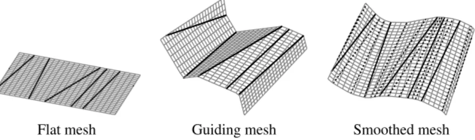
Generating a surface mesh using our model has two main steps. First, we bend a flat mesh around ‘guiding rules’. Second, we smooth its curvature using interpolated ‘extra rules’, as illustrated in Figure 2. The resulting mesh is piecewise planar. It is guaranteed to be admissible, in the sense that the underlying surface is developable.
Step 1: Bending with guiding rules. A ruled surface is defined by a differentiable
space curveα(t) and a vector fieldβ(t), with t in some interval I, see e.g. [11]. Points on
the surface are given by:
X(t,v) =α(t) + vβ(t), t ∈ I v ∈ R β(t) 6= 0. (1)
The surface is actually generated by the line pencil (α(t),β(t)). This formulation is
continuous.
Since our surface is represented by a mesh, we only need a discrete system of rules (sometimes named generatrices), at most one per vertex of the mesh. Keeping all possible rules leads to a model with a high number of parameters, most of them being redundant due to surface smoothness. In order to reduce the number of parameters, we use a subset of rules: The guiding rules. Figure 2 (left) shows the flat mesh representing the surface with the selected rules. We associate an angle to each guiding rule and bend the mesh along the guiding rules accordingly. Figure 2 (middle) shows the resulting guiding mesh. The rules are choosen such that they do not to intersect each other, which corresponds to the modeling of smooth deformations.
Step 2: Smoothing with extra rules. The second step is to smooth the guiding mesh.
To this end, we hallucinate extra rules from the guiding ones, thus keeping constant the number of model parameters. This is done by interpolating the guiding rules. The folding angles are then spread between the guiding rules and the extra rules, details are given in the next section. Figure 2 (right) shows the resulting mesh.
Flat mesh Guiding mesh Smoothed mesh
Figure 2: Surface mesh generation. (left) Flat mesh with guiding rules (in black). (middle) Mesh folded along the guiding rules. (right) Mesh folded along the guiding and extra rules.
2.2 Parameterization
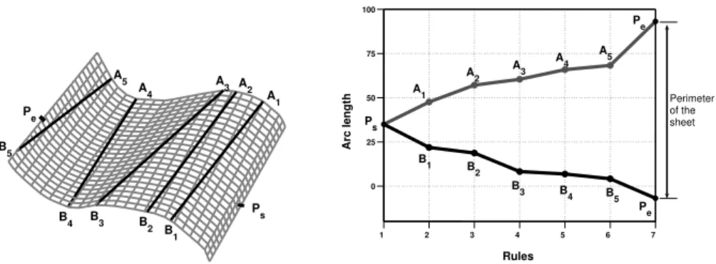
A guiding rule i is defined by its two intersection points Aiand Biwith the mesh boundary.
Points Aiand Bithus have a single degree of freedom each. A minimal parameterization
is their arc length along the boundary space curve. Since the rules do not intersect each
other on the mesh, we define a ‘starting point’ Ps and an ‘ending point’ Pesuch that all
rules can be sorted from Ps to Pe, as shown on Figure 3 (left). Points Ai (resp. Bi) thus
have an increasing (resp. decreasing) arc length parameter. The set of guiding rules
is parameterized by two vectors sA and sB which contain the arc lengths of points Ai
and Birespectively. The non intersecting rules constraint is easily imposed by enforcing
As explained above, the model is smoothed by adding extra rules. This is done by interpolating the guiding rules. Two piecewise cubic Hermite interpolating polynomials
are computed from the two vectors sAand sB. They are called fAand fB. This interpolation
function has the property of preserving monotonicity over ranges, as required. Figure 3
(right) shows these functions and the control points sAand sB. The bending angles are
interpolated with a spline and rescaled to account for the increasing number of rules.
Pe Ps A1 A2 A3 A4 A5 B5 B4 B3 B 2 B1 1 2 3 4 5 6 7 0 25 50 75 100 Arc length Perimeter of the sheet Rules Ps Pe Pe A1 A2 A3 A4 A5 B5 B4 B3 B2 B1
Figure 3: (left) The generated mesh with the control points (Ai,Bi). (right) Arc lengths sA
and sBof the control points with the interpolating functions fAand fB.
Table 1 summarizes the model parameters. The model has 4 + S + 3n parameters, S being the number of parameters describing the mesh boundary (for instance, width and height in the case of a rectangular shape) and n being the number of guiding rules.
Parameters Description Size
n number of guiding rules 1
ne number of extra rules 1
S mesh boundary parameters S
Ps arc length of the ‘starting point’ 1
Pe arc length of the ‘ending point’ 1
sA arc lengths of the first point defining the guiding rules n
sB arc lengths of the second point defining the guiding rules n
θ bending angles along the guiding rules n
Table 1: Summary of the model parameters. (top) Discrete parameters (kept fixed during nonlinear refinement step). (bottom) Continuous parameters.
The deformation is parameterized by the guiding rules. Those are sorted from the ‘starting point’ to the ‘ending point’, making wavy the deformation.
We define a directrix as a curve on the surface that crosses some rules once. A min-imal comprehensive set of directrices has the least possible number of directrices such that each rule is crossed by exactly one directrix. It is obvious that this set is reduced to a single curve for our model, linking the ‘starting point’ to the ‘ending point’. Conse-quenctly surfaces requiring more than one directrix can not be generated by our model, as for example a sheet with the four corners pulled up. The model however shows to be experimentally very effective.
3 A Multiple View Fitting Algorithm
Our goal is to fit the model to multiple images. We assume that a 3D point set and camera pose have been reconstructed from image point features by some means. We use the reprojection error as an optimization criterion. As is usual for dealing with such a nonlinear criterion, we compute a suboptimal initialization that we iteratively refine.
3.1 Initialization
We begin by reconstructing a surface interpolating the given 3D points. A rule detection process is then used to infer our model parameters.
Step 1: Interpolating surface reconstruction. Details about how the 3D points are
reconstructed are given in §4.1. The interpolating surface is represented by a 2D to 1D Thin-Plate Spline function [2], mapping some planar parameterization of the surface to point height. Defining a regular grid on the image thus allows us to infer the points on the 3D surface. Figure 4 and Figure 6 show two examples.
Step 2: Model initialization by rule detection. The model is initialized from the 3D
surface. The side length is choosen as the size of the 3D mesh.
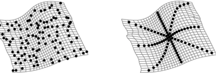
Guiding rules must be defined on the surface. This set of n rules must represent the surface as accurately as possible. In [3] an algorithm is proposed to find a rule on a given surface. It is a method that tries rules on several points on the surface with varying direction. We use it to compute rules along sites lying on the diagonal, the horizontal and the vertical axes. These sites are visible on Figure 4.
Figure 4: Model initialization. (left) Reconstructed 3D points and the interpolating sur-face. (right) Points where rules are sought.
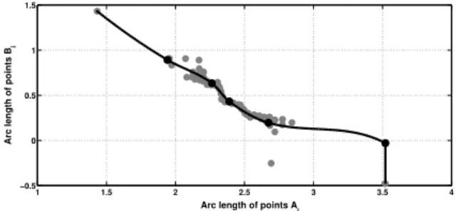
The rules are described by the arc length of their intersection points with the mesh
boundary. The two arc lengths defining a rule i can be interpreted as a point Ri in R2,
as shown in Figure 5 . Our goal is now to find the vectors sA and sB which define the
guiding rules, such that their interpolating functions fA and fB, defining the parametric
curve ( fA,fB)in R
2, describe the rules. We thus compute s
Aand sBsuch that the distance
between the curve ( fA,fB)and the points Riis minimized. We fix the number of guiding
rules by hand, but a model selection approach could be used to determine it from the set of rules.
This gives the n guiding rules. The bending angle vector θ is obtain from the 3D
surface by assuming it is planar between two consecutive rules. The initial suboptimal model we obtain is shown on Figure 6.
1 1.5 2 2.5 3 3.5 4 −0.5 0 0.5 1 1.5
Arc length of points B
i
Arc length of points Ai
PSfrag replacements Arc length of points Bi
Figure 5: The points in gray represent the detected rules. The black curve is the parametric
curve ( fA,fB)and the black points are the estimated controls points that define the initial
rules.
3.2 Refinement
The reprojection error describes how well the model fits the actual data, namely the image feature points. We thus introduce latent variables representing the position of each point onto the modeled mesh with two parameters. Let L be the number of images and N the number of points, the reprojection error is:
e =
∑
N i=1 L∑
j=1 (mj,i−Π(Cj,M(S,xi,yi))) 2 . (2)In this equation, mj,iis the i-th feature point in image j,Π(C,M) projects the 3D point M
in the camera C and M(S,xi,yi)is a parameterization of the points on the surface, with S
the surface parameters. The points on the surface are initialized by computing each (xi,yi)
such that their individual reprojection error is minimized, using initial surface model. To minimize the reprojection error, the following parameters are tuned: The parame-ters of the model (the number of guiding and extra rules is fixed), see Table 1, the pose of the model (rotation and translation of the generated surface) and the 3D point parameters. The Levenberg-Marquardt algorithm [5] is used to minimize the reprojection error. Upon convergence, the solution is the Maximum Likelihood Estimate under the assump-tion of an additive i.i.d. Gaussian noise on the image feature points.
4 Experimental Results
We demonstrate the representational power of our fitting algorithm on several sets of images. First, we present the computation of a 3D point cloud. Second, we show the results for the three objects we modeled. Third, we propose some augmented reality illustrations.
4.1 3D Points Reconstruction
The 3D point cloud is generated by triangulating point correspondences between several views. These correspondences are obtained while recovering camera calibration and pose using Structure-from-Motion [5]. Points off the object of interest and outliers are removed by hand. Figure 4 shows an example of such a reconstruction.
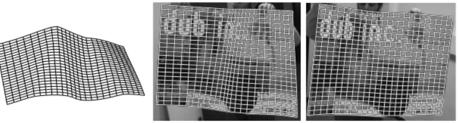
Figure 6: (top) 3D surfaces. (bottom) Reprojection into images. (left) Interpolated sur-face. (middle) Initialized model. (right) Refined model.
4.2 Model Fitting
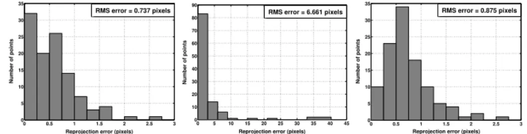
Even if our algorithm deals with several views, the following results have been performed with two views. Figure 6 and Figure 7 show the 3D surfaces, their reprojection into im-ages and the reprojection errors distribution for the paper sequence after the three main steps of our algorithm: The reconstruction (left), the initialization (middle) and the refine-ment (right). Although the reconstruction has the lowest reprojection error, the associated surface is not satisfying, since it is not enough regular and does not fit the borders of the sheet. The initialization makes the model more regular, but is not enough accurate to fit the boundary of the paper, so that important reprojection errors remain. At last, the refined model is visually acceptable and its reprojection error is very close to the reconstructed one. It means that our model accurately fits the image points, while being governed by a much lower number of parameters than the set of independant 3D points has. More-over the reprojection error significantly decreases thanks to the refinement step, which validates relevance of this step.
0 0.5 1 1.5 2 2.5 3 0 5 10 15 20 25 30 35
Reprojection error (pixels)
Number of points RMS error = 0.737 pixels 0 5 10 15 20 25 30 35 40 45 0 10 20 30 40 50 60 70 80 90
Reprojection error (pixels)
Number of points RMS error = 6.661 pixels 0 0.5 1 1.5 2 2.5 3 0 5 10 15 20 25 30 35
Reprojection error (pixels)
Number of points
RMS error = 0.875 pixels
Figure 7: Reprojection errors distribution for the images shown in Figure 6. (left) 3D point cloud. (middle) Initial model. (right) Refined model.
We have tested our method on images of a poster. The results are shown in Figures 8. The reprojections of the computed model are acceptable: The reprojection error of the reconstruction is 0.35 pixels and the one for the refined model is 0.59 pixels.
At last, we fit the model to images of a rug. Such an object does not really sat-isfy the constraints of developable surfaces. Nevertheless, it is stiff enough to be
well-Figure 8: Poster mesh reconstruction. (left) Estimated Model. (middle) Reprojection onto the first image. (right) Reprojection onto the second image.
approximated by our model. The results are thus slightly less accurate than for the paper and the poster: The reprojection error of the reconstruction step is 0.34 pixels and the one of the final model is 1.36 pixels. Figure 9 shows the reprojection of the model onto the images used for the reconstruction.
Figure 9: Rug mesh reconstruction. (left) Estimated Model. (middle) Reprojection onto the first image. (right) Reprojection onto the second image.
4.3 Applications
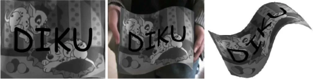
We demonstrate the proposed model and fitting algorithm by unwarping and augmenting images, as shown on Figures 10 and 11. Knowing where the paper is projected onto the images allows us to change the texture map or to overlay some pictures. The augmenting process is described in Table 2. Since we estimate the incoming lighting, the augmented images look realistic.
AUGMENTING IMAGES
1. Run the proposed algorithm to fit the model to images
2. Unwarp one of the images chosen as the reference one to get the texture map 3. Augment the texture map
4. For each image automatically do
4.1 Estimate lighting change from the reference image 4.2 Transfer the augmented texture map
Figure 10: Some applications. (left) Unwarped texture map of the paper. (middle) Chang-ing the whole texture map. (right) Augmented paper.
Figure 11: Augmentation. (left) Augmented unwarped texture map. (middle) Augmented texture map in the first image. (right) Synthetically generated view of the paper with the augmented texture map.
5 Conclusion and Future Work
This paper describes a quasi-minimal model for paper-like objects and its estimation from multiple images. Although there are few parameters, the generated surface is a good approximation of smoothly deformed paper-like objects. This is demonstrated on real image sequences thanks to a fitting algorithm which initializes the model first and then refines it in a bundle adjustment manner.
There are many possibilities for further research. The proposed model could be em-bedded in a monocular tracking framework or used to generate sample meshes for a learning-based model construction.
We currently work on alleviating the model limitations mentioned earlier, namely handling a general boundary shape and the comprehensive set of feasible deformation.
References
[1] V. Blanz and T. Vetter. Face recognition based on fitting a 3D morphable model.
IEEETransactions on Pattern Analysis and Machine Intelligence, 25(9), September
[2] F. L. Bookstein. Principal warps: Thin-plate splines and the decomposition of
deformations. IEEE Transactions on Pattern Analysis and Machine Intelligence,
11(6):567–585, June 1989.
[3] H.-Y. Chen and H. Pottmann. Approximation by ruled surfaces. Journal of Compu-tational and Applied Mathematics, 102:143–156, 1999.
[4] N. A. Gumerov, A. Zandifar, R. Duraiswami, and L. S. Davis. Structure of appli-cable surfaces from single views. In Proceedings of the European Conference on Computer Vision, 2004.
[5] R. I. Hartley and A. Zisserman. Multiple View Geometry in Computer Vision. Cam-bridge University Press, 2003. Second Edition.
[6] Y. Kergosien, H. Gotoda, and T. Kunii. Bending and creasing virtual paper. IEEE
Computer Graphics & Applications, 14(1):40–48, 1994.
[7] S. Leopoldseder and H. Pottmann. Approximation of developable surfaces with cone spline surfaces. Computer-Aided Design, 30:571–582, 1998.
[8] M. Pilu. Undoing page curl distortion using applicable surfaces. In Proceedings of the International Conference on Computer Vision and Pattern Recognition, Decem-ber 2001.
[9] H. Pottmann and J. Wallner. Approximation algorithms for developable surfaces. Computer Aided Geometric Design, 16:539–556, 1999.
[10] M. Salzmann, S. Ilic, and P. Fua. Physically valid shape parameterization for monoc-ular 3-D deformable surface tracking. In Proceedings of the British Machine Vision Conference, 2005.
[11] M. Sun and E. Fiume. A technique for constructing developable surfaces. In Pro-ceedings of Graphics Interface, pages 176–185, May 1996.