HAL Id: hal-01654890
https://hal.inria.fr/hal-01654890
Submitted on 5 Dec 2017
HAL is a multi-disciplinary open access
archive for the deposit and dissemination of
sci-entific research documents, whether they are
pub-lished or not. The documents may come from
teaching and research institutions in France or
abroad, or from public or private research centers.
L’archive ouverte pluridisciplinaire HAL, est
destinée au dépôt et à la diffusion de documents
scientifiques de niveau recherche, publiés ou non,
émanant des établissements d’enseignement et de
recherche français ou étrangers, des laboratoires
publics ou privés.
Improving time-series rule matching performance for
detecting energy consumption patterns
Maël Guilleme, Laurence Rozé, Véronique Masson, Cérès Carton, René
Quiniou, Alexandre Termier
To cite this version:
Maël Guilleme, Laurence Rozé, Véronique Masson, Cérès Carton, René Quiniou, et al.. Improving
timeseries rule matching performance for detecting energy consumption patterns. DARE 2017
-5th International Workshop on Data Analytics for Renewable Energy Integration, Sep 2017, Skopje,
Macedonia. pp.59-71, �10.1007/978-3-319-71643-5_6�. �hal-01654890�
Improving time-series rule matching
performance for detecting energy consumption
patterns
Ma¨el Guillem´e1,2, Laurence Roz´e1, V´eronique Masson1, C´er`es Carton2, Ren´e
Quiniou1, and Alexandre Termier1
1 Universit´e Rennes 1, INSA, INRIA / IRISA, Rennes, France
2 Energiency, Rennes, France
Abstract. More and more sensors are used in industrial systems (ma-chines, plants, factories...) to capture energy consumption. All these sen-sors produce time series data. Abnormal behaviours leading to over-consumption can be detected by experts and represented by sub-sequences in time series, which are patterns. Predictive time series rules are used to detect new occurrences of these patterns as soon as possible. Standard rule discovery algorithms discretize the time series to perform symbolic rule discovery. The discretization requires fine tuning (dilemma between accuracy and understandability of the rules). The first promis-ing proposal of rule discovery algorithm was proposed by Shokoohi et al, which extracts predictive rules from non-discretized data. An impor-tant feature of this algorithm is the distance used to compare two sub-sequences in a time series. Shokoohi et al. propose to use the Euclidean distance to search candidate rules occurrences. However this distance is not adapted for energy consumption data because occurrences of pat-terns should have different duration. We propose to use more ”elastic” distance measures. In this paper we will compare the detection perfor-mance of predictive rules based on several variations of Dynamic Time Warping (DTW) and show the superiority of subsequenceDTW.
1
Introduction
Nowadays, only around 60% of energy resources purchased by industrial enter-prises are used to create added value. The remaining 40% are considered to be lost. To trace these losses, companies are more and more equipped with sensors. Detecting dysfunctions from times series recorded by these sensors becomes a crucial problem for reducing energy consumption.
Dysfunctions can often be associated with specific patterns in time series (dysfunction signatures related to specific shapes of the time series). Thus, diag-nosing the abnormal behavior of an observed system, machine, or plant, could be achieved by locating patterns related to dysfunctions in time series. Our aim is to get typical patterns from experts (a pattern is a sub-sequence of a time series
II
selected by the expert) and to return the smallest prefix to detect, efficiently and as soon as possible, new occurrences of this typical pattern in a time series. Predictive rules discovery is adapted to this task. A predictive rule has two parts: one is called antecedent and the other consequent. It means that if the antecedent is recognized, the consequent will occur before a delay. These predic-tive rules are easily understandable for the expert. Our goal is to discover such predictive rules in time series for detecting power consumption problems.
Classical predictive rule discovery algorithms discretize time series data [3][7][19]. But discretization is a difficult task and requires to choose the appropriate dis-cretization method and to fine tune its parameters. To avoid this problem, in [15], Shokoohi et al. propose to extract predictive rules directly from time se-ries without discretizing data. Shokoohi et al.’s approach can be summarized as follows. Recurrent sequences are selected in a pre-processing step. Each of these sequences is split into two parts: an antecedent and a consequent. The split positions are chosen arbitrarily to yield a set of candidate rules. Then, for each rule, its occurrences, as pairs (antecedent, consequent), are retrieved in the time series, by that we call time series rule matching. These occurrences are used to compute a score for the rule, via a score function inspired by MDL[12] (Minimum Description Length). Finally the rule with the best score is returned. Shokoohi et al.’s algorithm makes use of the Euclidian Distance for time series rule matching. However, the Euclidian Distance does not cope with distortions on the time axis (called here time elasticity) which is often the case with power consumption data.
We study the use of different extensions [18][17][11] of Dynamic Time Warp-ing (DTW), a well-known distance measure [2], able to handle time elasticity, i.e. distortion in time. In this paper, we compare the performance (prediction early-ness and precision) of time series rules elaborated with three different distance measures, the Euclidean distance, DTW and subsequenceDTW [11].
Section 2 defines important concepts such as predictive rules and rules oc-currences. Section 3 presents some related works. Section 4 presents our method for time series rule matching. In section 5, we detail experiments for evalu-ating the performance of time series rule matching on a manually annotated energy-consumption time series, and according to three distance measures: the Euclidean distance used in [15], the DTW and subsequenceDTW, proposed as improvements.
2
Background
Sensors are used to capture energy consumption and to produce time series data. We consider here a time series T as defined in [5].
Definition 1: time series
A time series T is an ordered sequence of n real-valued variables T = (t1, ..., tn), ti∈
III
An expert gives a typical pattern to be searched. Such a pattern is a sub-sequence of a time series. In order to detect the pattern as soon as possible in time series, a predictive time series rule is built from the expert pattern.
Definition 2: predictive time series rule
A predictive time series rule R for a pattern p =< p1, ..., pk > is a pair (Ra, Rc).
The antecedent is Ra =< p1, ..., pi >. The consequent is Rc =< pi+1, ..., pk >.
It means that if the antecedent is recognized, the consequent will occur before a delay.
From a time series, an expert is able to extract a set of sub-sequences con-sidered similar. In energy consumption data, two similar sub-sequences can last longer or shorter. A pattern is shown in figure 1a and one of its occurrences is shown in figure 1b. As one can see, the occurrence is not identical to the searched pattern, both in duration and shape, but the expert still consider them as similar.
(a) searched pattern (b) an occurrence of the pattern
Fig. 1: Example of an occurrence (b) lasting shorter than the searched pattern (a) and having its bottom spike slightly shifted to the left.
The rules discovery algorithm is based on the similarity of two sub-sequences. Different parameters are needed: a distance measure D between two sub-sequences, a constant th (threshold of similarity), and a maxlag (maximum delay between the antecedent and the consequent of a rule).
Definition 3: Similarity of two sub-sequences
Two sub-sequences s1 and s2 are similar if and only if D(s1, s2) ≤ th. Definition 4: Set of occurrences of a sub-sequence in a time series
In a time series t =< t1, t2, ..., tn>, a set of occurrences O = {otii}i∈ST ART of a
sub-sequence s =< s1, s2, ..., sk > is the set of all sub-sequences oi similar to s
in t. ST ART [1..K] is the index of the occurrences where K is the length of O. oti
i =< ti, . . . , ti+li > is the i
th sub-sequence of s in t of size l
i starting at the
time ti with li∈ [1, n].
IV
A set of non overlapping occurrences of a sub-sequence in a time series t is a set of occurrences O such as ∀i, j ∈ ST ART , i < j ⇒ tj > ti+ li.
The former definitions are related to occurrences of sub-sequence. But, in rule discovery, these definitions can be extended to the case of occurrences of time series rules.
Definition 6: Set of rule occurrences
Let R = (Ra, Rc) a time series rule, t a time series and maxlag a positive
con-stant. A set of rule occurrences of R in t is a set ORwhere OR= {(ata11, c tc1 1 ), . . . , (a tam m , c tcm m )}. Let Oa = {ata11, . . . , a tam m } and Oc = {ctc11, . . . , c tcm
m } two sets of sub-sequence
occurrences, OR verify the following properties:
- Oa is a set of non overlapping occurrences of Ra in t.
- Oc is a set of non overlapping occurrences of Rc in t.
- ∀i ∈ [1, m], 0 < tci− tai+ lai< maxlag with lai the length of atai i.
- Oa∪ Oc is a set of non overlapping occurrences.
3
Related Work
Most approaches for discovering rules in real-valued time series rely on dis-cretization of time series in order to apply symbolic rule discovery methods [1]. A classical method, in [3], proposes to apply K-means clustering on time series to obtain symbolic data. This preprocessing step has been commonly used in several other rule discovery methods, as in [6], [7], [8]. However, clustering sub-sequences in time series can be unsuitable [9]. A single sub-sequence can occur several times in a cluster with narrow delays. This is called trivial matches [10]. In [14] and [19], Piecewise Linear Aggregation (PLA) is used as discretization method, but Shokoohi et al. show in [15] that this method is not adapted to rule-based prediction. Recently, Shokoohi et al. propose a discovery rule method which does not rely on a symbolic approach. This method is based on time series rule matching, consisting in finding rule occurrences in a time series (see section 2). Algorithms of time series rely on a distance measure for comparing series.
Distance measures Many distance measures exist but we focus here on mea-sures able to handle similarity with distortion in time (see section 2). In [4], Ding et al. compare various elastic distance measures. The accuracy of Dynamic Time Warping (DTW) is one of the best methods and requires few parameters.
DTW is a method for speech recognition, brought to the data mining com-munity in [2]. DTW is based on a dynamic programming approach to align two sequences and computes the optimal distance between them. Several extensions of DTW exist: FastDTW [13] speeds up its computation, OBE-DTW [18] and ψ-DTW [17] relax constraints on the endpoints of compared series. Another ex-tension, subsequenceDTW (subDTW) [11] finds several occurrences of a series in a time series in a single pass. Section 4.2 provides further details on DTW and subDTW.
V
4
Distance measures for time series rule matching
This section describes how a time series rule is matched on a time series. Then, we present in further details two existing elastic distance measures: DTW and subDTW.
4.1 Time series rule matching
Time series rule matching allows to find the occurrences of a time series rule in a time series. First a time series rule R is generated from the searched pattern s in the same way as in [15]. The searched pattern s is split into two parts: the first part is the antecedent Raand the last part is the consequent Rc(see section
2).
Time series rule matching is divided into two steps:
– step 1: identify all the antecedent occurrences Ra in the time series
– step 2: for each antecedent occurrence found in step 1, search the associated consequent Rc between this antecedent and the next one
Two steps are needed to retrieve first the sets of non-overlapping occurrences of the antecedent Ra. In both step 1 and 2, the search requires to compare
an-tecedent or consequent with a sub-sequence of the time series. Different param-eters are needed: a maxlag (the maximum length allowed between antecedent and consequent), a distance measure, a distance threshold, and for many dis-tance measures, a sliding window to browse all the sub-sequences of the time series. Intuitively, the distance threshold should only authorize small distance values, because the smaller is the distance the most similar the compared series are.
The maxlag is an expert knowledge and the choice of the distance measure D will be discussed later in section 4.2. A single distance measure is used for the search of antecedent and consequent occurrences. However, since the antecedent and the consequent can have different sizes, a specific threshold distance and a specific window size are required for each of them. We called tha (thc) the
distance threshold and wa(wc) the window size for the search of the antecedent
Ra (consequent Rc).
To avoid asking a user too many values, tha, thc, waand wcare automatically
computed from pth and pwindow. pth is a given percent of the distribution of
possible distance values between Ra (Rc) and sub-sequences of time series. pth
is easier to set than raw distance values. pwindowis a percent of the length of the
series searched (respectively Raand Rc). This parameter depends of the distance
measure D. For example if D is the Euclidean distance the value of pwindowmust
be 100% because Euclidean distance can only be calculated between series of the same size.
Algorithm 1 shows the time series rule matching. Step 1 is described by line 4, step 2 from line 5 to line 11.
During step 1, the window of size wa is slided at every successive position
VI
Algorithm 1 Time series rule matching
Input: distance measure D, time series rule R, time series ts, maxlag between an-tecedent and consequent, parameter for the window sizes pwindow, parameter for
the thresholds pth
Output: OR the set of occurrences of R in ts
1: OR, Oa← ∅ // Oa is the set of antecedent occurrences found
2: wa, wc← get window sizes(R, pwindow)
3: tha, thc← get thresholds distance(R, pth, wa, wc)
4: Oa← get antecedent occurrences(R, ts, D, wa, tha)
5: for all occa∈ Oa do
6: consequent ← get consequent(R, ts, D, maxlag, wc, thc)
7: if consequent f ound then
8: occR← create rule occ(occa, consequent)
9: OR.add(occR)
10: end if 11: end for 12: return OR
is compared to the antecedent Ra. If the distance is less than the threshold tha
the position gives a candidate match. During this matching, we need to ensure that no trivial matches are returned [10] (see section 3).
During step 2, for each antecedent occurrence found in step 1, the best can-didate match of Rc is retrieved. The best candidate must not overlap the next
antecedent occurrence. The delay between the current antecedent and this con-sequent must not exceed the maxlag.
As defined in section 2, during the search of the antecedent an consequent occurrences, the distance measure must be able to compare series with distortion in duration. The next section presents two existing distances measures handling this problem: DTW and subDTW.
4.2 Distance measures
The definition of DTW, given in [17], is used. To compute the optimal non-linear alignment between a pair of time series X and Y , with lengths n and m respectively, DTW typically bounds to some constraints: boundary condition, monotonicity condition and continuity condition. Many alignments satisfy all the conditions. DTW performs a dynamic programming algorithm to compute the alignment between X and Y with minimum cost (DTW distance). The time and space complexities are O(nm).
Here, X is the rule antecedent Ra or consequent Rc whereas Y is a
sub-sequence of a time series. To get a set of Y , DTW requires a sliding window browsing the time series. However, this raises a new problem, how to well con-figure the size of the window ? Indeed, a window too small could prevent to miss occurrences longer than the window, whereas a window too long, could cover several occurrences.
VII
One extension of DTW, subDTW [11], proposes to solve the setting of the window. It is a distance measure, which offers the aligning property of DTW without the boundary condition. Moreover, it does not need any window. For a more detailed presentation refers to [11]. The integration of subDTW to our time series rule matching algorithm allows to remove wa and wc during the search of
the antecedent and consequent occurrences.
5
Experimental results
The experiment consists of comparing three distance measures (the Euclidean distance, DTW and subDTW) to match 20 generated rules in an energy-consumption time series annotated by an expert. This expert knowledge is provided by the French start-up Energiency, a provider of software analyzing energy-consumption to improve energy performance. In section 5.2, the ability of each distance mea-sure to retrieve the annotated rule occurrences is evaluated. In section 5.3, the accuracy of distance measures is given with their related false alarm rate.
5.1 Experimental setup
The experiments are made on a real energy-consumption time series, called TS. Its frequency is ten minutes and its length is 26253 data points, which represents 6 months of energy consumption. The monitored system is an industrial plant composed of several machines. This kind of time series is commonly observed by experts.
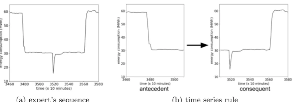
The expert is asked to pick a sub-sequence of TS related to a interesting phenomenon to predict. Figure 2a shows a sequence of an abrupt decrease, a steady state, a down spike, a steady state and an abrupt return to the initial steady state. As presented in section 4.1, a set of time series rules is first gen-erated by splitting the sequence at n equidistant points. A rule is gengen-erated for each split point. To avoid extreme rules (for example, a time series rule with an antecedent with only one data point), the minimum length of the antecedent and consequent parts is set at 5% of the length of the sequence picked by the expert. In our experiment, the number of divisions is set to 19, that yields a set of 20 rules, and one of these rules is illustrated in figure 2b.
For the experiment, the time series is manually annotated by an expert, ac-cording to the set of rules. As illustrated in figure 3, an annotation is an interval (fig. 3a). For the expert, a rule occurrence must start in this interval to be consid-ered as a match (fig 3b). In T S, 48 intervals are identified for each rule generated from the 1th, 2th, 3th, 19th and 20th split points. 65 intervals are found for each rule generated from the other split points. For each experiment, several values are tested for maxlag ({0h, 20h, 40h, 120h}) and pth({5%, 10%, 15%, 20%}). For the
Euclidean distance, pwindow is set to 100%, and for DTW, the values of pwindow
VIII
(a) expert’s sequence (b) time series rule
Fig. 2: Example of a rule (b), generated from the 8thsplit point in the expert’s
sequence (a).
(a) an annotated interval (b) a rule occurrence
Fig. 3: Correct matching example of an annotated occurrence (light hatching for antecedent, heavy hatching for consequent).
5.2 Performance of rule matching
In this experiment, the ability of each distance measure to retrieve the annotated rule occurrences is evaluated for the 20 rules generated. Let Actual True (T ) be the set of rule occurrences annotated in the time series T S by the expert, and Predicted True (P T ) the set of rule occurrences found by the rule matching algorithm where P T = {e|e ∈ T P ∪ F P }, True Positive T P = {e|e ∈ P T ∩ T } and False Positive F P = {e|e ∈ P T \T }. Precision Pr and recall Rc are then computed as follows:
P r =|T P ||P T | = |T P ∪F P ||T P | Rc = |T P ||T |
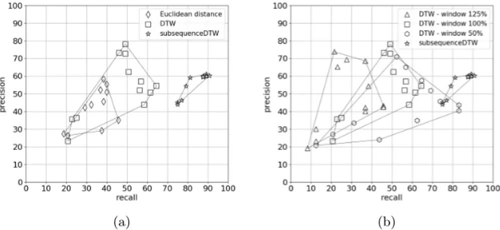
Figure 4a shows the precision versus the recall for the three distance mea-sures: the Euclidean distance, DTW and subDTW. The results of each distance measure are surrounded by a convex hull (covering the results for the 20 rules).
IX
Surrounding the results allow to compare more easily the global performance for each distance measure. Note, that a small convex hull implies a small variation in performance among the 20 rules.
The results confirm that the Euclidean distance is not adapted to retrieve rule occurrences with time distortion. Indeed, the Euclidean distance compare series point-to-point without relying on an alignment algorithm. Moreover, only series with the same size can be compared. The precision of DTW is at least as high as the precision of subDTW, but the convex hulls show that the performance of DTW strongly varies according to the rule. SubDTW has a better recall than DTW, thus more annotated rule occurrences are found.
Figure 4b shows the impact of the size of the sliding window on the per-formance of DTW. When the size of the window increases, the recall decreases. Whereas if the size of the window decreases, then the recall increases but the pre-cision decreases. These results confirm that most of the annotated occurrences of the rules in T S are shorter than the rule. Moreover, if the size of the window is too large, no consequent are found in T S because the antecedent occurrence overlaps the entire rule occurrence. Defining the correct size of the window is critical for the performance of DTW. Several sizes of window can be tested but the execution time is strongly impacted.
This problem does not concern subDTW, because a window is not required. The recall of subDTW is higher than the recall of DTW for any size of the window. The use of subDTW to perform time series rule matching is best suited to time series with distortion in duration for rule occurrences.
Note that, after the experiments, the values of pthis set to 20% and maxlag
is set to 120 hours, which represents 5 days. The maxlag is high because the time series are associated to an industrial environment, where breakdowns and maintenance can take several days.
(a) (b)
Fig. 4: Precision/recall plots for Euclidean, DTW and subDTW distances (a) and DTW with several window sizes (b).
X
5.3 False alarms rate
The next experiment focuses on the accuracy of the distance measure, according to the false alarm rate measured by the confidence. Let Incomplete Predicted True (IP T ), the set of the antecedent occurrences found by the time series rule matching algorithm IP T = {e|e ∈ T P ∪ F P ∪ A} with A the set of antecedent occurrences found without consequent. The confidence Cf can be computed as follows:
Cf = |IP T ||P T | = |T P ∪F P ∪A||T P ∪F P |
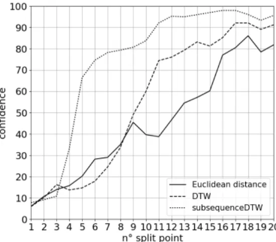
Figure 5 shows the confidence of each distance measure for the 20 rules gener-ated. SubDTW has a higher confidence than DTW and the Euclidean distance, especially between the 4th split point rule and the 10th split point rule. Thus,
subDTW triggers less false alarms.
Fig. 5: Confidence plot for Euclidean, DTW and subDTW distances
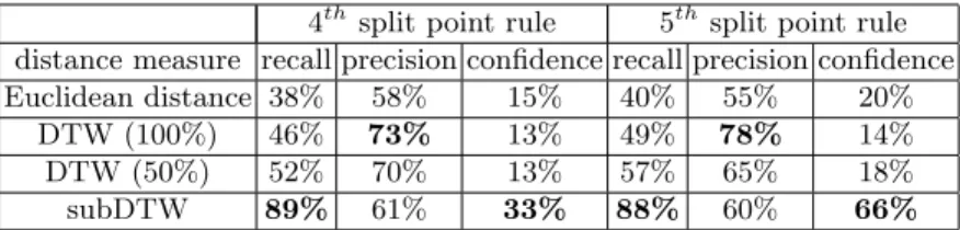
Table 1 presents the confidence, the recall and the precision for the 4th and the 5thsplit point rules. These split point rules have a small antecedent allowing to predict sooner the searched pattern. SubDTW keeps a good ratio between precision, recall and confidence for rules with a small antecedent.
6
Conclusion and future research
We have investigated time series rule matching in a rule discovery algorithm in energy consumption time series. In this context, time series rule matching must compare sub-sequences with distortion in time. We evaluate three existing
XI
Table 1: Recall, precision and confidence for 4th and 5thsplit point rules. Bold
numbers highlight the best result in each column.
4thsplit point rule 5thsplit point rule distance measure recall precision confidence recall precision confidence
Euclidean distance 38% 58% 15% 40% 55% 20%
DTW (100%) 46% 73% 13% 49% 78% 14%
DTW (50%) 52% 70% 13% 57% 65% 18%
subDTW 89% 61% 33% 88% 60% 66%
distance measures on a real use case: the Euclidean distance used in [15], DTW a well-known elastic measure and subDTW, an extension of DTW which does not require a sliding window to browse the time series. The results confirm that the Euclidean distance is not adapted to find rule occurrences with different du-ration. Whereas, DTW and subDTW can handle the task. However, subDTW allows to find occurrences of rule with smaller antecedent, without losing per-formance. Finding occurrences of rule with small antecedent means predicting energy consumption problems ”as soon as possible”. Furthermore, subDTW does not need to set a sliding window.
There are lot of avenues for future work. We primarily focused on the con-straint brought by using a sliding window when taking into account the duration of the occurrences in time series rule matching. However, as with all the methods relying on a distance measure, setting the right threshold is a very important and difficult task. That is even more important in our case, because we work from the shape which is highly dependent of the expert judgment. That’s why we pro-pose to explore interactive learning, to learn the threshold by asking the expert to evaluate a sub-set of occurrences found, then to iterate until an acceptable threshold was found.
We remind that time series rule matching is only a step of the rule discov-ery algorithm. In [15], time series rule matching is used to find occurrences of candidate rules. The score of each candidate rule is computed, from these oc-currences, by a score function inspired by MDL. This score function works only for rule occurrences with the antecedent and consequent of the same duration of the candidate rule. With our new time series rule matching which find rule oc-currences with different length this condition doesn’t hold anymore and require to find a new score function.
In the presented rule discovery algorithm, a whole rule is generated from a sequence given by an expert. However, the given sequence could be only used for the antecedent or consequent part of the rule. Then, the algorithm has to find in time series the other part of the rule.
A last avenue can be to extend rule discovery to a set of time series as proposed in [15]. The distance measures have to be adapted to multiple time series, but there is already a proposal in [16].
XII
References
1. R. Agrawal, T. Imieli´nski, and A. Swami. Mining association rules between sets of items in large databases. In Acm sigmod record, volume 22, pages 207–216. ACM, 1993.
2. D. J Berndt and J. Clifford. Using dynamic time warping to find patterns in time series. In KDD workshop, volume 10, pages 359–370. Seattle, WA, 1994.
3. G. Das, K. Lin, H. Mannila, G. Renganathan, and P. Smyth. Rule discovery from time series. In KDD, volume 98, pages 16–22, 1998.
4. H. Ding, G. Trajcevski, P. Scheuermann, X. Wang, and E. Keogh. Querying and mining of time series data: experimental comparison of representations and dis-tance measures. Proceedings of the VLDB Endowment, 1(2):1542–1552, 2008. 5. P. Esling and C. Agon. Time-series data mining. ACM Computing Surveys
(CSUR), 45(1):12, 2012.
6. S. K Harms, J. Deogun, and T. Tadesse. Discovering sequential association rules with constraints and time lags in multiple sequences. In International Symposium on Methodologies for Intelligent Systems, pages 432–441. Springer, 2002.
7. M. L. Hetland and P. Sætrom. Temporal rule discovery using genetic programming and specialized hardware. In Applications and Science in Soft Computing, pages 87–94. Springer, 2004.
8. X. Jin, Y. Lu, and C. Shi. Distribution discovery: Local analysis of temporal rules. In Pacific-Asia Conference on Knowledge Discovery and Data Mining, pages 469– 480. Springer, 2002.
9. E. Keogh, J. Lin, and W. Truppel. Clustering of time series subsequences is mean-ingless: Implications for previous and future research. In Data Mining, 2003. ICDM 2003. Third IEEE International Conference on, pages 115–122. IEEE, 2003. 10. J. Lin, E. Keogh, S. Lonardi, and P. Patel. Finding motifs in time series. In Proc.
of the 2nd Workshop on Temporal Data Mining, pages 53–68, 2002.
11. M. M¨uller. Information retrieval for music and motion, volume 2. Springer, 2007. 12. J. Rissanen. Modeling by shortest data description. Automatica, 14(5):465–471,
1978.
13. S. Salvador and P. Chan. Toward accurate dynamic time warping in linear time and space. Intelligent Data Analysis, 11(5):561–580, 2007.
14. P. Sang Hyun, W. Wesley, et al. Discovering and matching elastic rules from sequence databases. Fundamenta Informaticae, 47(1-2):75–90, 2001.
15. M. Shokoohi-Yekta, Y. Chen, B. Campana, B. Hu, J. Zakaria, and E. Keogh. Dis-covery of meaningful rules in time series. In Proceedings of the 21th ACM SIGKDD International Conference on Knowledge Discovery and Data Mining, pages 1085– 1094. ACM, 2015.
16. M. Shokoohi-Yekta, B. Hu, H. Jin, J. Wang, and E. Keogh. Generalizing dtw to the multi-dimensional case requires an adaptive approach. Data Mining and Knowledge Discovery, 31(1):1–31, 2017.
17. D. F. Silva, G. E. A. P. A. Batista, E. Keogh, et al. On the effect of endpoints on dynamic time warping. In SIGKDD Workshop on Mining and Learning from Time Series, II. Association for Computing Machinery-ACM, 2016.
18. P. Tormene, T. Giorgino, S. Quaglini, and M. Stefanelli. Matching incomplete time series with dynamic time warping: an algorithm and an application to post-stroke rehabilitation. Artificial intelligence in medicine, 45(1):11–34, 2009.
19. H. Wu, B. Salzberg, and D. Zhang. Online event-driven subsequence matching over financial data streams. In Proceedings of the 2004 ACM SIGMOD international conference on Management of data, pages 23–34. ACM, 2004.