Active control of tiltrotor blade in-plane loads during maneuvers

ACTIVE CONTROL OF TILTROTOR BLADE IN-PLANE

LOADS DURING

MANEUVERS

by

David George Miller

B.S. in Aerospace Engineering, Penn State University. (1983),

M.S. in Mechanical Engineering, Drexel University. (1986) SUBMITTED TO THE DEPARTMENT OF

AERONAUTICS AND ASTRONAUTICS IN PARTIAL FULFILLMENT OF THE REQUIREMENTS FOR THE

DEGREE OF MASTER OF SCIENCE

at the

MASSACHUSETTS INSTITUTE OF TECHNOLOGY May 1988

Copyright (c) 1988 Massachusetts Institute of Technology

Signature of Author v

Y' v LJpuululllL . v.

-onautics

and Astronautics

May 27, 1988

Certified by

Professor Norman D. Ham Thesis Supervisor

Accepted by

IIf-w

-

/7

(,/ . Professor Harold Y. Wachman..

A r -, . .. -. , -.

Aegro

CB'j~~ an'~~tllaen.-Thesis ' z Committee

WITHDRAWN

MAY 2 4 1988 LIRiES

. d~s

1 tnoAwDI

LOADS DURING

MANEUVERS

by David G. Miller

Submitted to the Department of Aeronautics and Astronautics on June 3, 1988 in partial fulfillment of the requirements for the degree of Master of

Science.

Abstract

The origin of one/rev rotor aerodynamic loads which arise in tiltrotor aircraft during airplane-mode high speed pull-up and push-over maneuvers is examined using a coupled rotor/fuselage dynamic simulation. A modified eigenstructure assignment technique is used to design a controller which alleviates the in-plane loads during high pitch rate maneuvers. The controller utilizes rotor cyclic pitch inputs to restructure the aircraft short period and phugoid responses in order to achieve the coupling between pitch rate and rotor flapping responses which minimizes the rotor aerodynamic loading. Realistic time delays in the feedback path are considered during the controller design. Stability robustness in the presence of high frequency modelling errors is ensured through the use of singular value analysis.

Thesis Supervisor: Title:

Professor Norman D. Ham

Dedication

To Dr. Norman Ham, whose patience and guidance made this work possible; the Boeing Helicopter Company, for funding my stay at MIT; and Jim White, for his technical advice on the subject of tiltrotor simulation.

Table of Contents

Abstract 2 Dedication 3 Table of Contents 4 List of Figures 5 List of Tables 6 1. Introduction 7

1.1 Motivation for Research 7

1.2 Previous Research 9

1.3 Scope of Research 13

2. Mathematical Model Description 14

2.1 Introduction 14

2.2 Exponential Basis Function Technique 14

2.3 Tilt Rotor Modelling Points 17

3. Physics of In-Plane Loads In Tiltrotors At High Speeds 22

3.1 Introduction 22

3.2 Derivation of Out-of-Plane Precessional Moment Equations 22 3.3 Derivation of In-Plane Moment Equations 26

3.4 Intuitive Concepts 32

4. Eigenstructure Assignment Methodology 41

4.1 Introduction 41

4.2 Eigenstructure Analysis 42

4.3 Formulation of Closed-Loop Eigenvalue Problem 46 4.4 Solving for the Achievable Eigenvectors 49

4.5 Finding the Feedback Gains 51

5. The Rotor In-Plane Moment Controller 60

5.1 Introduction 60

5.2 Consideration of Cyclic Pitch Authority Limits 60

5.3 Design of Phugoid Eigenvector 61

5.4 Controller Evaluation 68

6. Conclusions 79

References 81

List of Figures

Figure 1-1: Artist's Conception of Commercial Tiltrotor 8

Figure 3-1: Gimbal Axis System 23

Figure 3-2: Relative Wind And Airfoil Geometry 27

Figure 3-3: Open-Loop Longitudinal Stick Step Responses 33

Figure 3-4: Rotor Flapping Responses During Tiltrotor High Speed Pull-Up 36 Maneuver

Figure 3-5: Longitudinal Stick Step Responses for Pitch Rate to Elevator 38 Feedback Controller

Figure 3-6: Block Diagram of Combined Elevator and Rotor Cyclic Pitch 40 Controller

Figure 4-1: Closed-Loop Longitudinal Stick Step Responses When Short Period 57 Mode is Shaped to Minimize In-Plane Loads

Figure 4-2: Comparison of Cumulative In-Plane Loads Produced by 59

Longitudinal Stick Step Input for Pitch Rate to Elevator Feedback and Short Period Mode Shaping Controllers

Figure 5-1: Closed-Loop Longitudinal Stick Step Responses for Reduced 62 Authority In-Plane Loads Controller

Figure 5-2: Closed-Loop Longitudinal Stick Step Responses For Finalized 66 Combined Elevator and Rotor Cyclic Pitch Controller

Figure 5-3: Comparison of Longitudinal Stick Step In-Plane Loads Responses 71 for Various Controller Configurations

Figure 5-4: Stability Robustness Test for Finalized In-Plane Loads Controller 72

Figure 5-5: Bode Magnitude Plot of Output Sine Component of In-Plane Loads 74 Produced by Longitudinal Stick Input

Figure 5-6: Longitudinal Stick Step Responses For In-Plane Loads Controller 75 Using Only Rigid Body Feedback Gains

Figure 5-7: Effect of Rotor State Feedback Gains on In-Plane Loads Bode 77 Magnitude Plot

List of Tables

Table 2-I: Tiltrotor Open-Loop Modes at 260 Knots 20 Table 2-1: Description of Simulation State Variables 21 Table 4-I: Open-Loop and Desired Short Period Eigenvectors for In-Plane 47

Loads Reduction

Table 4-11: Desired and Achievable Short Period Eigenvectors for In-Plane 52 Loads Reduction

Table 4-111: Feedback Gains for In-Plane Loads Minimization 56

Table 5-I: Finalized Closed-Loop Short Period and Phugoid Eigenvectors 65

Table 5-II: Finalized In-Plane Loads Controller Feedback Gains 69

Table 5-1I: Finalized Closed-Loop Eigenvalues 70

Table A-I: Rotor Properties 84

Chapter 1

Introduction

1.1 Motivation for Research

The tiltrotor aircraft offers the advantages of low speed operability and vertical take-off or landing capability of a helicopter, while providing the efficiency and comfort of high speed airplane mode flight. The tiltrotor aircraft can potentially fulfill a wide variety of commercial, military, and law enforcement missions. Presently, however, most proposed tiltrotor applications have been in the air transport category. The agility offered by the tiltrotor design has not been fully exploited, in part because of concern about high rotor loads encountered during aggressive maneuvers.

This thesis will focus on the development of in-plane rotor loads in the tiltrotor during high speed, airplane-mode, pitch axis maneuvers. The level of in-plane bending moments exerted on the rotor blades has been shown [1] to be the limiting factor of g capability of the tiltrotor aircraft. The stiff in-plane rotor configuration which is proposed for most tiltrotor designs allows no inertial relief of the blade in-plane moments through lagging motion of the rotor blade about a lag hinge. As a result, in-plane moments exerted on the rotor blade result directly in yoke chord bending moments. If the yoke chord bending moments exceed the structural limit load of the blade, severe damage to the rotor system may occur.

The objective of this.research is twofold. First the origin of the in-plane loads in high speed flight will be investigated. Second, an understanding of the physics of the phenomenon will be used to propose a means of alleviating the in-plane loads problem. It is shown that a firm physical explanation of the dynamics of the in-plane loads, together with the sophisticated computer-aided control system design software available today, can produce a feasible solution to the problem.

1.2 Previous Research

The maneuverability and agility characterisitcs of the tiltrotor aircraft are discussed in a paper by Schillings et. al. [1], wherein the authors show that blade one/rev in-plane loads in high speed flight are directly related to aircraft pitch rate. An advanced pitch axis controller is developed in [1] which effectively limits the maximum transient pitch rate attainable by the aircraft in response to pilot commands. The solution presented in [1] essentially uses feedback of aircraft pitch rate to the elevator to produce a closed-loop pitch rate response to disturbances and pilot inputs which is smaller, both in transient and steady state conditions, than the open-loop response. Although the ref. [1] controller limits the relative magnitude of aircraft pitch rate, the amount of in-plane moment for a given magnitude of pitch rate is basically unaltered by pitch rate feedback to the elevator.

The study conducted in [1] uses several mathematical models to predict the aircraft behavior. A nonlinear coupled rotor/fuselage analysis (C81) [2] is compared to the generic tiltrotor simulation (GTRS) program [3], an analysis which is used primarily for real-time piloted simulation. Comparison of both analyses with flight test [1] shows a high degree of fidelity in predicting the in-plane loads during pitch axis maneuvers. The GTRS model uses nonlinear fuselage equations of motion coupled with linear rotor flapping equations, in which only the lower frequency rotor flapping dynamics are approximated by coupled first order lags, to represent the in-plane loads phenomenon. The high degree of fidelity achieved by the linearized rotor model in representing flight test behavior indicates that a linear rotor model can adequately represent the pertinent dynamics of the in-plane loads phenomenon. It has also been shown [4] that linearized rigid body aircraft models can accurately model aircraft behavior for single axis pitch rate maneuvers up to very high pitch rates and and high angles of attack. As a result, a linear, coupled rotor/fuselage analysis can be used to simulate the in-plane loads dynamics.

During helicopter-mode flight, the aircraft relies on swashplate inputs to provide the forces and moments necessary to control the aircraft. During transitional flight from helicopter-mode to airplane-mode flight a combination of swashplate and airframe control surface inputs, including flap, aileron, rudder, and elevator deflections, are used to control the aircraft. In high speed airplane-mode flight, the tiltrotor relies entirely on airframe control surface deflections to provide acceptable handling qualities. Recent studies [5,6] indicate that active control of helicopter blade motion through swashplate inputs can provide gust alleviation, vibration suppression, and flapping stabilization in helicopters. Thus active control of the rotor blades through swashplate inputs in airplane-mode flight will be considered as a means to alleviate the in-plane loads.

This thesis will concern itself with the control of a three bladed rotor system, wherein the method of multiblade coordinates [7] can be used to eliminate the periodicity from the coupled rotor/fuselage equations of motion. The resulting linear constant coefficient system will include the cyclic and collective pitch angles of the rotor blades as the control input terms. It is shown by Ham [8] that there is an equivalence between active one/rev control using a conventional swashplate arrangement, relying on lateral and longitudinal cyclic pitch and collective pitch, and individual blade actuation for a three bladed rotor system. As a result, the methodologies developed for control and estimation of the rotor blade motion within the scope of individual-blade-control (IBC) research may be applied to the problem. _{Therefore one can use appropriately filtered blade mounted sensor} information [9] to provide an accurate estimate of rotor blade motion.

Several powerful design methodologies exist for the control of multivariable linear systems. Generally, these design techniques can be categorized as either time domain or frequency domain approaches. Frequency domain methods use graphical techniques to characterize system performance as a function of input command or disturbance frequency, while time domain techniques characterize performance in terms of the time responses of the variables of interest in the system.

Command following and controller robustness issues are addressed in the frequency domain by the well known Nyquist and Bode gain and phase plots in the single-input-single-output case, and by the analogous maximum and minimum singular value plots verse frequency in the multivariable case [10]. Although applied more naturally to control system performance analysis, frequency domain techniques can be adapted for use in controller design. A model based compensator [11] can be used to perform an approximate inverse of the plant dynamics, replacing the unfavorable frequency domain characteristics of the plant with the desirable characteristics of some dynamic model. In general the model based compensator requires a dynamic compensator of order equal to the order of the plant. The implementation of a model based compensator may therefore not be feasible from a practical standpoint for high order systems.

Another frequency domain approach is the use of H-Infinity design methodology, in which shaping of the maximum singular values of various system frequency response matrices is employed to ensure adequate performance and robustness [12]. The use of the singular value, the measure of multivariable robustness, as an index of performance allows for an extremely elegant and powerful parametrization of the class of all stabilizing controllers. The process of extracting from the class of stabilizing controllers the specific controller which best satisfies the design objectives is presently a topic of research. Techniques have been formulated [13] for the solution to the H-Infinity problem when the controller and plant are represented in the form of a model based compensator. The software required to solve the H-Infinity problem for the model based compensator representation has only recently been developed [13], and is not yet generally available to the engineering community.

Linear Quadratic Regulator (LQR) theory considers the mimimization of the sum of the weighted deviation of the system states and controls from some desired trajectory, integrated over an arbitrary time interval [14]. The resulting LQR controller consists of

constant gain linear feedback of all the system states to all the sytem controls. In order to apply LQR design to a given problem, one must consider a specific desired trajectory and have access to all the system states. The frequency domain characteristics of the controller are not easily specified in the LQR design methodology. As a result, stability robustness issues involving high frequency sensor noise or unmodelled dynamics, usually most easily described in the frequency domain, are not readily addressed by LQR theory.

An alternative time domain design approach is eigenstructure assignment [15], wherein constant gain output feedback is used to assign the system closed-loop poles and right eigenvectors. A great deal of insight into the sytem dynamics is required to make an appropriate choice of the desired eigenvalues and eigenvectors. A poor choice of the desired eigenstructure may result in a system which exhibits unacceptable performance, execessive control usage, or poor robustness characteristics. For systems in which the phenomenon of interest is associated with a particular dynamic mode, and there exists sufficient knowledge to make an appropriate choice of eigenstructure, the eigenstructure assignment approach can be used to address both time and frequency domain criteria. Also, the design need not be optimized for a specific type of input because the form of the right eigenvectors will shape the system response for any set of initial conditions or control inputs.

As mentioned previously, the in-plane loads have been shown to be directly related to the aircraft pitch rate. The rapid rotation of the airplane in pitch is predominantly due to the dynamics of the short period mode [16]. As a result, appropriate phasing of the rotor and airframe responses during the short period response presents a possible means of alleviating the in-plane rotor loads.

The aircraft angle of attack and pitch rate responses are dictated by handling qualities criteria. Thus knowledge of the desired short period pole location, and desired phasing of the aircraft angle of attack and pitch rate responses will be taken as a given for this analysis.

A controller which modifies the eigenstructure in the low frequency range, while leaving higher frequency modes unchanged, should be robust to high frequency modelling errors. Thus by designing a controller which modifies only the short period dynamics, which occur in the vicinity of one cycle per second, robustness to modelling errors of the higher frequency rotor dynamics, which occur above four cycles per second, can be ensured.

1.3 Scope of Research

An overview of the coupled rotor/fuselage model used to represent the tiltrotor aircraft is presented in chapter 2. The simulation model includes six degree of freedom rigid body motion and rotor flapping dynamics. Cyclic pitch actuator dynamics are modelled as a 0.1 second time delay using Pade approximations. The combination of rigid body, rotor, and actuator dynamics results in a state space description of the aircraft which contains 29 states.

An explanation of the relationship between in-plane loads and aircraft pitch rate in the tiltrotor in high speed, airplane-mode flight is offered in chapter 3. Basic aerodynamic and mechanical principles are exploited to yield a tractable expression for the in-plane loads in terms of the system state variables. The one/rev in-plane loads are shown to be a function of rotor cyclic flapping and blade pitch angles, and aircraft pitch rate and angle of attack.

Chapters 4 and 5 describe the controller design process. Chapter 4 reviews eigenstructure assignment methodology using constrained state feedback. A controller is then developed which minimizes in-plane moments by properly phasing aircraft rigid body motion, rotor cyclic flapping, and cyclic pitch inputs. Chapter 5 then considers adapting the controller design to operate within realistic cyclic pitch authority limits.

Chapter 2

Mathematical Model Description

2.1 Introduction

A mathematical model of the aircraft should be sufficiently sophisticated to represent the pertinent dynamics of the in-plane loads. The math model should not, however, be so detailed as to hopelessly complicate the control system design process. Powerful control system design techniques exist for linear time invariant (LTI) systems, therefore a linearized model is developed which represents the in-plane loads in the frequency range of interest. A description of the generic modelling algorithm used to represent the tiltrotor aeromechanical characteristics is given in the following sections.

2.2 Exponential Basis Function Technique

The task of formulating a representative rotor/fuselage mathematical model has always been complicated by the large number of coordinate transformations necessary to define the rotor position and orientation in inertial space. The algebra involved in the derivation of the simplest rotor model is formidable, making manual derivation of the equations tedious and prone to error. In order to minimize the human effort involved in the derivation process, thereby reducing the risk of modelling errors, it is necessary to utilize a computer-aided modelling algorithm.

One possible alternative to the tedious manual algebra is the use of a symbolic algebraic manipulation program, such as MACSYMA [17], to perform the required calculations. Unfortunately, the derivation of the equations of motion for a three or four degree of freedom system using MACSYMA requires several minutes of CPU time using a

mainframe computer, while generating literally dozens of pages of fortran code. A typical helicopter dynamic model may require three degrees of freedom to describe the aircraft rigid body pitch, roll, and yaw motions, another two degrees of freedom to describe the rotor shaft tilt relative to the body axis system, and finally three degrees of freedom to describe the rotor blade azimuth, flapping, and geometric pitch angles. The derivation of the resulting eight degree of freedom math model requires a prohibitive amount of CPU time and memory storage using MACSYSMA, even for a powerful mainframe computer. In addition, changes in the aircraft configuration require a complete rederivation of the symbolic equations of motion. To the best of the author's knowledge, the symbolic generation of a representative helicopter flight dynamics simulation has not yet been

accomplished.

A second approach to mechanizing the derivation process is to calculate the numerical value of terms in the equations of motion, while ignoring the symbolic interpretation of the terms. The resulting numerical values of the terms in the equations of motion can then be calculated with much greater speed and much less computer storage than their symbolic equivalents. Gibbons and Done (18) used the computer to eliminate some of the labor involved in deriving a set of equations for studying aeroelastic stability. Purely numerical algorithms, such as the one developed by Gibbons and Done, require costly and computationally complex numerical differentiation procedures to obtain the coefficients of the acceleration and velocity terms which appear in the equations of motion. In addition, linearization of the equations requires numerical perturbation techniques. A disadvantage of casting the equations of motion in purely numerical form is some loss of intuition into the physical processes which underlie the system dynamics. One cannot directly examine the symbolic expressions for the coefficients of any of the variables in the equations of motion.

methods discussed above. The task of deriving the equations of motion which involve many coordinate transformations can be simplified if the position vectors, describing the location of all the mass elements in the system, can be written in a form which can be easily manipulated. The underlying idea is to express the coordinate transformations required in the math model in a structure which is easily retained throughout each phase of the derivation process.

One of the operations which complicates the derivation of the equations of motion is axis transformation from one coordinate system to another. Coordinate transformations are most easily accomplished by means of multiplication of transformation matrices, where each transformation matrix represents a rotation about a particular coordinate axis. It can be shown [19] that the elements of all transformation matrices can be written as a summation of exponential functions whose arguments consist only of the coordinate transformation angles. Multiplication of the coordinate transformation matrices results in

addition of the arguments of the exponential functions. A second operation which yields great algebraic complexity is the time differentiation of the position vector to obtain the velocity and acceleration terms in the equations of motion. Linearization can also be accomplished by partial differentiation of the nonlinear equations of motion with respect to the state variables to obtain the coefficients of the state variables in the dynamic equations. As a result, formulation of the position vector in terms of exponential basis functions, perhaps the simplest functions to differentiate, also simplifies the derivation process. The reader is referred to [19] for a complete treatment of the exponential basis function (EBF) simulation generation process.

23 Tilt Rotor Modelling Points

A single rotor helicopter simulation based on the exponential basis function algorithm has been favorably correlated with flight test data (19). In light of the correlation of the exponential basis function simulation and flight test data, it is reasonable to assume that the coupled rotor/fuselage equations derived for the tiltrotor aircraft using the EBF algorithm have a high degree of fidelity. Although there are many similarities in the general structure of the tiltrotor and single rotor helicopter defining equations, there are several differences in the two types of vehicles which necessitate modification of the math model generation software. The most significant of these software modifications are described below.

The gimballed rotor configuration of the tiltrotor is represented in the math model by a modified, low hinge offset, articulated rotor system. The gimbal is represented by modifying the multiblade coordinate flapping equations by adding a relatively small cyclic flapping spring term to the cyclic flapping equations, and a large coning spring term to the coning equations. The cyclic flapping spring represents the effect of the gimbal hub spring, while the coning spring represents the effect of blade flexibility. The simulation can thus allow for motion of the tip path plane about the gimbal axes, as well as represent in-phase coning motion of the blades out of the gimbal plane. The advantage in this approach is to represent both the low frequency flapping due to gimbal motion and the higher frequency first harmonic flapping due to blade flexibility by using only three dynamic degrees of freedom. An exact representation of the gimballed rotor system requires two degrees of freedom to represent gimbal motion, and three more dynamic degrees of freedom to represent the out-of-plane bending of each of the three rotor blades.

Current tiltrotor designs utilize a constant speed joint to eliminate two/rev drive system loads [20]. The constant speed joint maintains constant rotational velocity in the

gimbal axis system, effectively aligning the rotor angular velocity vector in a direction normal to the gimbal plane. As a result, the rotor precesses in a manner similar to a rigid cone when undergoing cyclic flapping motion, engendering no blade one/rev chordwise coriolis moments. The action of the constant speed joint is taken into account by a separate derivation of the in-plane moment equations using Euler's equations of motion.

Displacement of the pitch housing relative to the swashplate is a result of the combined effect of gimbal tilt and blade flexibility. As a result, the blade pitch/flap coupling is itself a function of azimuth. In order to represent this phenomenon, the equations of motion were modified to account for different amounts of blade pitch change

due to cyclic flapping motion and coning motion.

The equations of motion of the single rotor helicopter simulation [19] had been represented in an inertial axis system. In keeping with standard airplane control system design practice, a transformation of coordinates to a stability [16] axis system was undertaken. The resulting equations of motion were then modified to account for

downwash perturbations on the horizontal tail induced by changes in wing lift.

The resulting linearized rotor/fuselage model contains twelve dynamic degrees of freedom. In addition to the six degrees of freedom of rigid body motion, there is a degree of freedom associated with the flapping motion of each of the three rotor blades on each of the aircraft's two rotors. The aircraft rigid body states included in the simulation are body axis pitch, roll, and yaw angular rates; Euler pitch, roll, and yaw angles; and integral and proportional body axis vertical, longitudinal, and lateral velocity states. Coleman coordinates are used to express the rotor equations in constant coefficient form, using lateral cyclic, longitudinal cyclic, and coning blade flapping angles and rates. Actuator dynamics are represented as pure time delays through Pade approximations. The Pade approximations introduce additional first order differential equations, wherein the elevator and rotor cyclic pitch angles are included as dynamic states, which increase the number of

state variables in the simulation to twenty-nine. Table 2.1 details the dynamic modes associated with the nominal 260 knot, aft center of gravity condition considered in this analysis. The numbering system used to reference each state in the model, and the physical units of each of the state variables, is given in Table 2.2.

MODE FREQUENCY

(rad/sec)

Symmetric Progressive Flap. -6.5 + 72.8i

Antisymnmetric Progressive Flap. -6.5 + 72.8i

Symmetric Coning -6.4 + 40.7i

Antisymmetric Coning -6.3 + 41.5i

Symmetric Regressive Flap. -7.0 + 28i

Antisymmetric Regressive Flap. -6.9 + 2.8i

Short Period -1.5 + 2.3i

Roll Convergence -1.7003

Dutch Roll -0.2 + 1.5i

Phugoid -0.1 + 02i

Spiral -0. 0569

Heading 0.0000

Integral Longitudinal Velocity 0.0000 Integral Vertical Velocity 0.0000

Elevator Actuator -20.000

Right Rotor Long. Cyclic Pitch Act. -20.000 Right Rotor Lat. Cyclic Pitch Act. -20.000

Left Rotor Long. Cyclic Pitch Act. -20.000

Left Rotor Lat. Cyclic Pitch Act, -20.000

Table 2-1: Tiltrotor Open-Loop Modes at 260 Knots

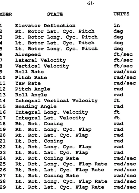
NUMBER STATE

1 Elevator Deflection

2 Rt. Rotor Lat. Cyc. Pitch 3 Rt. Rotor Long. Cyc. Pitch

4 Lt. Rotor Lat. Cyc. Pitch

5 Lt. Rotor Long. Cyc. Pitch

6 Airspeed 7 Lateral Velocity 8 Vertical Velocity 9 Roll Rate 10 Pitch Rate 11 Yaw Rate 12 Pitch Angle 13 Roll Angle

14 Integral Vertical Velocity

15 Heading Angle 16 Integral 17 Integral 18 Rt. Rot. 19 Rt. Rot. 20 Rt. Rot. 21 Lt. Rot. 22 Lt. Rot. 23 Lt. Rot. 24 Rt. Rot. 25 Rt. Rot. 26 Rt. Rot. 27 Lt. Rot. 28 Lt. Rot. 29 Lt. Rot. Long. Velocity Lat. Velocity Coning

Long. Cyc. Flap Lat. Cyc. Flap

Coning

Long. Cyc. Flap Lat. Cyc. Flap

Coning Rate

Long. Cyc. Flap Rate Lat. Cyc. Flap Rate

Coning Rate

Long. Cyc. Flap Rate Lat. Cyc. Flap Rate

Table 2-11: Description of Simulation State Variables

UNITS in deg deg deg deg ft/sec ft/sec ft / sec rad/sec rad/sec rad/sec rad rad ft rad

ft

ft

rad rad rad rad rad rad rad/sec rad/sec rad/sec rad/sec rad/sec rad/sec

Chapter 3

Physics of In-Plane Loads In Tiltrotors

At High Speeds

3.1 Introduction

Euler's equations of motion can be used to formulate the equations of motion of the gimballed rotor system. Fundamental mechanics and linear aerodynamics can then be used to derive the in-plane moments exerted on the rotor blades. The resulting equations contain a compact representation of the effect of rigid body aircraft motion, cyclic flapping, and rotor cyclic pitch inputs on in-plane rotor loads. The form of the in-plane moment equations allows for a physically satisfying explanation of some of the counter-intuitive aspects of tiltrotor behavior in high speed flight.

3.2 Derivation of Out-of-Plane Precessional Moment Equations

In order to precess the rotor at the aircraft pitch rate a net gyroscopic moment must be exerted on the rotor system. The precessional moment will be made up mainly of one/rev aerodynamic moments exerted on the rotor blades and partially by hub moments exerted by the gimbal spring restraint. Referring to Figure 3.1, Euler's equations of motion for the external moments exerted on the system can be written:

aa

=

.~

gf

+

IXA

(3.1)

M = E - x A

where A is the angular momentum vector expressed in the gimbal axis system, and o is the angular velocity of the gimbal axis coordinate system with respect to a fixed frame. The angular momentum in the gimbal frame is given by:

w=9 0 deg k-:gimbal k (shaft axis) k -gimbal k (shaft axis) yr=270 deg =180 deg i igimbal TOP VIEW F=0 deg i x=270 deg W Nf=180 deg FRONT VIEW

Figure 3-1: Gimbal Axis System

W=0 deg

imbal

a,

W

W

LEFT SIDE VIEW

T N'=9 0 deg -! I I i l

A = -3I A k (3.2)

Noting the assumed equivalence between cyclic flapping and gimbal motion, one can use the cyclic flapping expression

A = al cos

+

b

sin

(33)

to obtain the angular velocity of the gimbal frame with respect to a fixed frame of reference.

C q-7~ a1 )(3.4)

The constant speed joint ensures that when shaft RPM is constant the angular momentum in the gimbal axis system is conserved. Therefore, one can write:

-aAat

= o

(3.5)

Performing the cross-product operation in eqn. (3.1) yields the external moments exerted on the rotor system:

M = 3IfQ( Ca1)l + 3I Q(bl)i (3.6)

The external moments exerted on the rotor system will be composed of a combination of aerodynamic and hub moments. The moments exerted on the hub which result from the nth blade reacting against the gimbal spring restraint, resolved about the x

and y gimbal axes, are given by:

Mx = -K sin n

where K is the gimbal spring constant and

3

is the cyclic flapping angle. The total hub moments exerted by the gimbal spring are the result of the actions of each of the three rotor blades,

MX

n-

A-K

(a

1

cos n

+

b sin ) sin

i

(3. 8)

M = }

RK(al cos n +

b

sin

)cos

(3 9)

therefore:

Mx - -2 K bl

(3.10)

3

MY

-- K

a

1

The harmonic portion of the aerodynamic out-of-plane moments exerted on each rotor blade can now be expressed as:

M

T

=

EC

cos

n

+

M

S

sin n

(3.11)

The net gimbal axis moments exerted on the rotor system will be given by:

Mx = nil

TSi n

E

(3.12)

M = nl MT cos n = MTC

Adding the gimbal spring and plane aerodynamic moments yields the sum of out-of-plane moments equation:

K b +MT =3 (q-a)

(3.13)

3 3 3I

- K al + l3z b

Solving for the one/rev out-of-plane aerodynamic moments exerted on each blade gives:

S

_'S

- 21n2I(q-al)

_A

+

KRb

_{1 (3.14)}

Tc -= 2I a(bl ) + Kal

3.3 Derivation of In-Plane Moment Equations

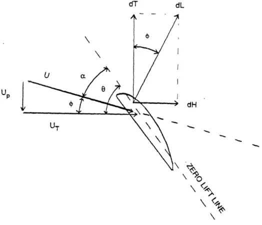
Now consider how the out-of-plane aerodynamic moments required to precess the rotor relate to the in-plane blade moments. Figure 3.2 shows the relative wind and airfoil geometry for the high inflow condition. One can neglect the aerodynamic drag forces on the rotor blade element to write the in-plane and out-of-plane aerodynamic forces exerted on the rotor as:

d = dL sin 0

(3.15)

dT = dL cos 0

where one can use the exact expression for thin airfoil lift due to angle of attack to obtain the lift force:

1 2

dL

.,/p

5

a c u sin (a) dr

(3.16)

For convenience, collect the air density, lift curve slope, differential radial element length, and blade chord length constants into one constant given by:

CA = . p a c dr (3.17)

First, in order to gain a general understanding of the relationship between H-force and thrust force in the tilt-rotor at high speed, consider only the aerodynamic forces at the three-quarter radius location. For the high inflow condition, the inflow angle will be on

dT

U

dL

dH

UT

Figure 3-2: Relative Wind And Airfoil Geometry

IO

the order of 45 degrees. Thus small angle approximations for the inflow angle are not valid. In airplane-mode flight the rotor operates as a propeller, generating only enough thrust to overcome the relatively small aerodynamic drag forces exerted on the aircraft. As a result, the lift produced by the rotor will be much smaller than the helicopter mode lift which is required to sustain the gross weight of the aircraft. Therefore, the angle of attack of the blade element, given by the difference of the blade geometric pitch angle 0 and the inflow angle, will be small and one can safely use small angle approximations for the -( term to obtain:

dE = CAU

2

(

-0 ) sin

(3.18)

T = CAU 2 ( -

0)

cos

Taking the variation of the in-plane and thrust forces gives:

6(dH) = [2CAU( - 0) sin 6U

+ ICAU

2

_{sin 0) (}

_-

₀₎

+

[CA

U2

_{(0 -}

_{) cos}

_0]

₆₀

(3.19)

d(dT) = [2CAU( - ) cos 0] 8U + [CAU 2 cos 0] ( - 60) + [ -CAU2 ( - 0) sin 0] 60

An order of magnitude analysis can be used to simplify the expressions above to include only the dominant terms:

d(dH) z [CAU2 sin ( - 60)

Inspection of the equations above reveals that the incremental thrust and H-force perturbations from trim are proportional and related by:

8(dH)/(dt)

= tan 0

(3.21)

The thrust and H-forces act through the same radial moment arm, therefore the incremental in-plane and out-of-plane aerodynamic moments contributed by the blade element are also proportional. The simplified expression above predicts that the ratio of the in-plane to out-of-plane aerodynamic moments increases as the airspeed, hence inflow angle, increases. The insight gained from the simplified three-quarter radius analysis is that a greater percentage of the required out-of-plane moment is exerted as a chordwise bending moment on each of the rotor blades as airspeed increases.

In order to obtain a more precise relationship between the in-plane and out-of-plane aerodynamic moments, a spanwise integration analysis is presented which accounts for the variation in rotor aerodynamic properties with radial location. Referring again to Figure 3.2, one can note:

sin = Up/U

(3.22)

cos = UT/U

One can therefore write the incremental thrust and H-forces by substituting eqns. (3.22) into eqns. (3.15) and (3.16):

dE

=

CAU2

_{sin ( -}

_{) p/U}

_(3.23)

d --= CAU 2 sin ( - ) UT/U

Using the trigonometric identities for the sine and cosine of the sum of two angles yields:

dB =CAUU

p

sin

cos

- cos 0 sin ]

(3.24)

Using the expressions for sin(c) and cos(4) from eqns. (3.22) gives:

dEl - CA [sin

U

-cos

T

UpU

ff

=

CA [sin troS

% J

The perturbation in-plane the variation of the above:

8(dE) =

+ [sin

+ [cos

and out-of-plane aerodynamic forces can be obtained by taking

CA {[sin Up] 8U

9 u

- 2 cos

9

Up)] U

0 UpUT + sin 0 Up2] )e}

(3.26)

6(d) = CA ([2 sin IUT - os Up)] UT

+ [-cos UT] SUp

+

[S

UT2 + sin

UpUT)]

80

One can use the approximate expressions for perturbation tangential and perpendicular relative wind velocities and geometric blade angle given below:

pU SUT 8e = r(~ -q cos ) = W sin = 9C COS + 91S Sin

(3.27)

to rewrite the perturbation integral thrust and H-force moment expressions, given below, in terms of the system state variables.

o =

R (dH) r

(3.28)

MT=

of

R (d

) r

Substituting the actual flight conditions and rotor geometry given in Appendix A into the expressions above, and then integrating the product of the radial moment arm and the incremental thrust and H-forces, yields the perturbation in-plane and out-of-plane aerodynamic moments. bM = (12032.46)

(I-q

cos ) + (901347.94) 60

+

(1030.53)(6W

sin )

(3.29) 6M_T = (14985.18) (f - q cos ) + (956760.61) 0

+

(1022.39)

(6W

sin i)

The expressions above indicate that the thrust and in-plane moment perturbations are very similar in form. In order to assess the differences in the expressions, subtract a multiple of the perturbation thrust moment from the perturbation in-plane moment to obtain:

E6M - 0. 8BMr = (133110) 6 + (209.59) W sin (3.30)

Remembering the expression derived for the aerodynamic out-of-plane moment in eqn.(3.14), one can express the in-plane moment as:

6MI = 0.8{[2(q-a₁) I + Kb ] sin

+

(133110)

6

+ 209.59 (6W sin )

(3.31)

+ [2b_lIf + K _{al] cos}

SMH

=

t0.8[2Ig

(q-al)

+ b1

(3.32)

+ 133110 0ls + 209.59 6W sin

+ 0.8[2IA ba + K al] + 133110 01c} cos i 3.4 Intuitive Concepts

Presented in Figure 3.3 is a time history of an open-loop aft longitudinal stick step at 260 knots. An order of magnitude analysis reveals that the most significant contribution to the in-plane moment is made by the term (q - al). As the aircraft pitches nose-up, the tip-path-plane actually leads the shaft angular velocity. This unusual behavior can be attributed to the unique operating conditions of the tiltrotor.

First consider the approximate relationships for incremental thrust and H-force of eqn. (3.20). The change in thrust and H-force is very nearly proportional to the change in angle of attack. For the case of fixed rotor blade pitch, the rotor will experience a change in angle of attack given by:

8a = - s - = [tan- 1(U /U

I p

iT

t

rat

T

u1

(3.33)

In a typical low inflow condition, the ratio of the trim out-of-plane velocity to the trim in-plane-velocity is small, thus angle of attack changes are due primarily to changes in the out-of-plane velocity. In the high inflow condition, however, the ratio of the tangential and perpendicular velocities is close to unity. As a result, changes in the tangential velocity can significantly change the blade section angle of attack.

Now consider the change in angle of attack at =90 degrees which gives rise to the longitudinal flapping response of the rotor. The change in tangential velocity for the high

0 2 4 TIME 6 IN SECONDS 21 18 (A 0 z r C. 15 12 9 6 0 -3 8 10 Figure 3.3A 0 2 4 6 TIME IN SECONDS Figure 3.3C 4 I/ a Z C. z a. rj UL U_C. C-2 0 -2 -4 -6 -8 -10 8 10 0 2 4 6 8 10 TIME IN SECONDS Frgure 3.3B 0 2 4 6 8 10 TIME IN SECONDS Figure 3.3D

Figure 3-3: Open-Loop Longitudinal Stick Step Responses -. 99 -.992 -. 994 w ₁ -.996 z -. 998 · Z -1 -1.002 Z -1.004 -1.006 -1.008 -1.01 4 (l 3 LJ 2 2 1 Z 0 0 -1 a -2 Z 0. -3 0. Ij -4 -_5 , -6 -7 ,...,-.,,,,,,-...

0 2 4 6 8 11 TIME IN SECONDS Figure 3.3E , , , I , - - I- - I I I I I · I , I 0 2 4 6 TIME IN SECONDS Figure 3.3G 3.9 3.6 3.3 <C 3 27 0 40 2.4 , 2.1 2 1.8 1.5 12 .9 2 8 10 35000 30000 v) I 25000 Z 20000 z u 15000 2 10000 LU I 5000 z 0 -5000 0 2 4 6 TI7ME IN SECONDS Fg ure 3.3F 2 4 6 TIME IN SECONDS Figure 3.3H Figure 3-3 , continued - - ---,, l ,,I I . I I . I . . . i . . 100 80 . 60 L-z 40 S 20 0 -O 0 un -20 -40 O -60 -80 -100 .01 m 008 (3 .006 w z .004 z < 0 ° - .002 z O -. 004 U- .006 -.008 -.01 8 10 8 10 SW I

speed pull-up maneuver is due largely to the body axis vertical velocity and given approximately by eqn. (3.27). At high speed, the change in the vertical body axis velocity is large. The change in the out-of-plane velocity is due primarily to longitudinal flapping and can be written:

6Up = - al

r sin

i

(3.34)

The change in angle of attack is given by:

bz = UT Up

(Up

ma

+U

₂

_~2

_{SW + al 9 r}

UT

_sin

(3.35)

Particularizing the expression above for the conditions at the three-quarter radius location and assuming that the ratio of the in-plane and out-of-plane velocities is unity gives:

ba = 1 S(W + al (0.75)R sin (3.36)

2 R (0.75)

The aerodynamic portion of the precessional moment for a nose-up pitch rate must be supplied by a positive angle of attack change at WN=90 degrees. The angle of attack change induced by the W velocity alone is greater than the angle of attack change needed to produce the precessional moment. As a result, a negative longitudinal flapping angle, corresponding to the tip path plane leading the shaft normal plane as the shaft pitches nose-up, is necessary to maintain moment equilibrium during the pull-up maneuver. As the body axis velocity W builds up during the maneuver, the longitudinal flapping angle becomes increasingly negative, hence a negative longitudinal flapping rate is produced.

The most significant term in the in-plane moment expression was shown to be given by:

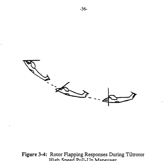
Figure 3-4: Rotor Flapping Responses During Tiltrotor High Speed Pull-Up Maneuver

The large body-axis vertical velocity induced by the pull-up maneuver at high speed and the high inflow condition of the rotor result in the curious effect of the pitch rate and tip path plane precessional rate occurring in the opposite direction. As a result the magnitude of the pitch rate and longitudinal flapping angular rate sum to give a large one/rev in-plane bending moment.

The one/rev in-plane moments have been shown to be a consequence of airplane pitch rate. Thus reducing the aircraft pitch rate whenever possible is one approach to alleviating the in-plane loads. Figure 3.5 illustrates the effect of pitch rate feedback to elevator angle, similar to the ref. [1] controller design, on the longitudinal stick step responses. The presence of this type of feedback results in smaller pitch rates, hence lower in-plane moments, than the open-loop responses.

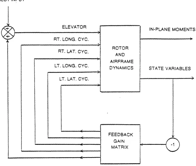
Rotor cyclic pitch inputs can be used to modify the angle of attack, and hence aerodynamic forces and moments, experienced by the rotor blades. Through modification of the one/rev aerodynamic forces and moments exerted on the blade, the optimum rotor flapping responses for in-plane loads reduction can be produced. Shown in Figure 3.6 is a block diagram of the combined rotor cyclic pitch and elevator controller which is to be examined in subsequent chapters. The controller utilizes feedback of the system state variables to the elevator, left rotor longitudinal and lateral cyclic pitch, and right rotor lateral and longitudinal cyclic pitch to alleviate the one/rev blade in-plane loads.

0 2 4-TIME Figure 6 IN SECONDS 3.5A 0 2 4 6 TIME IN SECONDS Figure 3.5C 14 12 (n CL 0 z

:

I

E. 10 8 6 4 2 0 -2 8 10 au 2 Z o -2 S -6 -8 8 10 0 2 4 6 TIME IN SECONDS Fligure 3.58 0 2 4 6 TIME IN SECONDS Figure 3.50

Figure 3-5: Longitudinal Stick Step Responses for

Pitch Rate to Elevator Feedback Controller -.99 - .992

-

.994 In w -. 996 U Z -.998 -1 ; -1.002 Z - 1.004 -1.006 -1 008 -1.01 , , , , I ., I, , , I , n o: w_a z 2 a z a EL CL 2 1.5 1 .5 0 -.5 -1 -1.5 -2 -2.5 -3 -3.5 8 10 8 10

-0 2 4 TIME IN F;gure 6 SECONDS 3.5E 0 2 4 6 'TIME IN SECONDS Figure 3.5G 2.5 2.4 0 z 0 o 2.2 2 1.8 1.6 1.4 1.2 .8 8 10 TIME IN SECONDS Figure 3.5F 8 O1 21000 m z w_O z UJ 18000 15000 12000 9000 6000 3000 0 -3000 0 2 4 6 'IIME IN SECDNDS Figure 3.5H Figure 3-5, continued ~~<8 W~~5 . U I , I ,, , I ,, , I .I I I , 50 40 (A 30 L. z 20 ° lO o 0 cn -10 x -40 -50 .01 u 008 LI w 2: o .005 w o .004 W .002 Z_J z < 0 ° -.002 0 -. 004 u -. 005 -.008 -.01 8 10 : - -

-PILOT INPUT 1 ELEVATOR RT. LONG. CYC. RT. LAT. CYC. LT. LONG. CYC. LT. LAT. CYC. IN-PLANE MOMENTS STATE VARIABLES J.t1

Figure 3-6: Block Diagram of Combined Elevator

and Rotor Cyclic Pitch Controller

ROTOR AND AIRFRAME DYNAMICS FEEDBACK GAIN MATRIX _ _t _ ,, , ~ , ~e --- - --- -__ v~. --- · ·- · I···I·--·I __ _= -_- ·111 - - .--- _ -- ,, ,, mir, i i J-- i ,i-- ,,, , , J,, , , , IICP·--LI ---- i _- _I

-

- ---I

0 r i ·-·----L····I·--L---C;· II

Chapter 4

Eigenstructure Assignment Methodology

4.1 Introduction

The optimal solution to the tiltrotor maneuvering loads problem is the design of a controller which drives the sine and cosine components of the in-plane moment expressions presented in eqn. (3.32) to zero. The in-plane loads arise as a function of the aircraft pitch rate and the ensuing increase in aircraft angle of attack. As a result, a controller which minimizes the aircraft pitch rate will ensure that the in-plane loads remain small. Unfortunately, it is sometimes necessary for the pilot to execute high pitch rate maneuvers in order to adequately perform his mission. As a result, the blade in-plane loads controller should be designed to satisfy the more stringent requirement of driving the loads toward zero even when the aircraft sustains a substantial pitch rate.

Constraints introduced by the physics of the rotor/airframe interaction, limits on the allowable blade flapping responses and cyclic pitch inputs, and time delays in the controller operation will define the achievable reduction in rotor loads. Additionally, the controller must be designed to operate in the presence of a wide variety of pilot inputs, many of which develop aggressive pitch rates. The problem considered here is to find the controller which minimizes the in-plane loads without adversely affecting the handling qualities of the

4.2 Eigenstructure Analysis

The response of a linear time invariant system expressed in the form:

x = Ax + Bu (4.1) is given by: k.t

x(

=

v

_i

_wi

_te

(4.2)

;, (t-')

+

t

1 UK.

() e

d}

where })i,vi, and w_i are respectively the eigenvalues, and the right and left eigenvectors of

the state matrix A; ~ is the initial state; and uk are the control inputs. For any combination of initial conditions and control inputs, the state response will be defined by the form of the right eigenvectors of the state matrix A. The relationship between the individual state responses will be determined by the magnitude of the components of each state in the eigenvectors of the system. If one desires a particular relationship between any set of states, the proper shaping of components of the eigenvector will ensure that the given relationship between the states is satisfied for any type of input or initial condition.

In order to minimize the one/rev in-plane moments a specific relationship must exist between the aircraft pitch rate, vertical body axis velocity, rotor cyclic pitch angles, and longitudinal and lateral flapping responses. To eliminate completely the one/rev in-plane aerodynamic moments, both the sine and cosine components of the right-hand side of eqn. (3.32) must equal zero. The two simultaneous equations which must be satisfied to eliminate the one/rev in-plane moments are given below.

0.8[2 I n(q-a) + KRb1 ]+ 133110 i1S + 209.59 W = 0

(4.3)

The high speed pull-up maneuver described in Fig. 3.3 is dominated by the short period response of the aircraft. Assuming that only the short period mode is excited during the maneuver, the relationship between the state vector and the time derivative of the state vector is given by:

X = ~sLp X (4.4)

where 4sp is the short period frequency. Generally, the short period frequency is specified by handling qualities requirements and is not a parameter which can be altered during the loads controller design. Similarly, the coupling between the aircraft pitch rate and body axis vertical velocity, hence angle of attack, are selected based upon handling qualities criteria. Thus treating q,SW, and LSp as known quantities, one can write eqn. (4.3) in matrix form. -0.16

I

-209.59

0

0~ I IWI

-

0

.

16

,

I

0

0.8K

0

133110

O

0 .Kg _I~~~~~~~~0.16PspI a 133110 0 a1

al

bi

Ia

L1S

(4.5)

M

=

Mb

i Mc]

1al

bi

els

The equation written above is overdetermined in that there is no unique combination of rotor cyclic flapping and cyclic control angles which yields zero in-plane loads.

Physically, however, the rotor control angles and blade flapping responses will not be independent for fixed values of pitch rate and vertical body axis velocity. An approximate relationship between the rotor flapping and cyclic control angles can be obtained through the quasi-static flapping assumption, wherein one assumes that the rotor flapping states reach a steady-state condition instantly.

The state vector can be partitioned into and the state equations rewritten in the form:

[: - I [22

rigid body and flapping degrees of freedom,

(4.6)

The quasi-static flapping approximation assumes that the time rates of change of the flapping states instantly approach zero, therefore:

= 0

(4.7)

The lower row of equations of eqn. (4.6) can then be solved algebraically, using the quasi-static flapping approximation, to give:

- 1 -1

i

x-122

B

2

u

(4.8)

For the flight conditions considered in this analysis, the following relationship exists between rotor cyclic flapping angles and cyclic control angles, body axis velocity w, and pitch rate: al + 1C

(b]

=L

+

MR1W1

1e Is

[0.84

-1.45]

0.144

11.46

0.82

t-o

.0507

-0.0016 1 (4.9)

0.00081 . B

i

Ui2

The expressions above have been derived under the assumption that the flapping state variables instantly reach steady-state values. In actuality, some finite time interval will elapse before the flapping dynamics decay and the blade lateral and longitudinal flapping angles reach the steady-state values predicted by eqn. (4.9). The phase relationship between rotor cyclic control inputs and aircraft state can be better represented by remembering that the lowest frequency fixed-frame flapping mode occurs at a complex

frequency of:

( -

A1)

= - 6.85 + 2.78j RAD/SEC

The time to reach steady-state conditions of these low frequency flapping dynamics is given roughly by the inverse of the undamped natural frequency of the regressive flapping mode:

= - 0.135 SECNDS

The desired short period frequency will be chosen as: isp = -3 + 3j RAD/SEC

Thus, if the effect of the flapping dynamics is represented by a pure time delay, the relationship between the rotor cyclic control inputs and aircraft pitch rate and vertical velocity states responding through the short period dynamics is given by:

[b]

= L [ML ] + M R

[t5

]

One can write the relationship between the cyclic flapping, rotor cyclic pitch, and aircraft rigid body states more succinctly as:

ab] : [

C

]

[ WI (4.10)

where: = e3 e3 j ML

After substituting the above into eqn. (4.5), and performing some simple matrix algebra, one can solve for the desired 1c and 1s participation factors in terms of the specified pitch rate and body axis vertical velocity participation factors from:

C

]=

[E

e

+Mat

[ M '

Iri

(w

(4.11)

The desired lateral and longitudinal flapping participation factors can then be found from eqn. (4.10).

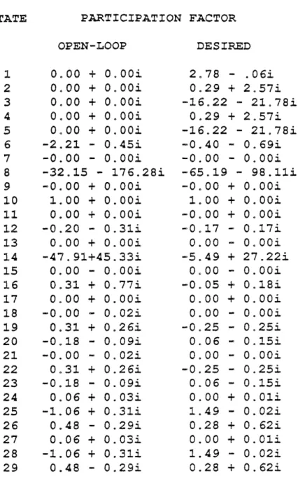
One can choose the desired closed-loop coning and airspeed participation factors to be equal to the open-loop values. The eigenvector which contains the desired coupling of the state variables is termed the "desired eigenvector". Table 4.1 compares the open-loop and desired short period eigenvectors for the tiltrotor in-plane loads reduction example. In reality, the physics of the system may make it impossible to use the available controls to achieve the form of the desired closed-loop eigenvector in an exact sense. An algorithm is described in the following sections which produces the controller which most closely approximates the desired eigenvector in a weighted least-squares sense.

4.3 Formulation of Closed-Loop Eigenvalue Problem

When a control of the form shown below is

u =

-Gx

+v (4.12)

used on the system of eqn. (4.1), the closed-loop state equations become:

EA -

G] x + y

(4.13)

PARTICIPATION FACTOR DES IRED OPEN-LOOP 0.,00 2 0 00 3 0.00 4 0.00 5 0,00 6 -2.21 7 -0.00 8 9 10 11 12 13 14 15 16 17 18 19 20 21 22 23 24 25 26 27 28 29 -32. 15 -0. 00 1. 00 0.00 -0.20 0.00 -47. 91 0. 00 0.31 0, 00 -0. 00 0,31 -0,18 -0. 00 0o31 -0.18

0.06

-1.06 0.48 0.06 -1. 06 0.48

+ 0.

00i

+ 0 . 00i + 0,OOi + 0o 00i + 0.OOi - 0.45i - 0.00i - 176.28i + 0.OOi + 0.OOi + 0.OOi - 0.31i

+ O.

00i

.+45.33i

-

000i

+ 0.77i

+ 0.OOi

- 0, 02i

+ 0.26i

- 0. 09i - 0 02i + 0.26i - 0.09i + 0.03i + 0.31i

- 0.29i

+ 0.03i + 0.31i - 0.29i 2.78 - .06i

0.29

+

257i

-16.22 - 21.78i 0.29 + 2,57i -16,22 - 21.78i

-0.40

- 0.69i

-0.00 - 0.OOi -65.19 - 98.11i -0.00 + 0.00i 1.00 + 0.OOi -0.00 + 0,OOi -0,17 - 0.17i

0.00 -

0.00i

-5.49 + 27.22i 0,00 - 0.OOi -0.05 + 0o18i 0,00 + 00OOi

0.00

- O.00i

-0.25 - 0,25i 0.06 - 0. 15i 0.00 - 0O. 0Oi -0.25 - 0.25i 006 - 0. 15i 0.00 + 0.01i

1.49 -

0.02i

0.28

+

0.62i

0.00

+ 0.01i

1.49 - 0.02i 0.28 + 0.62i

Table 4-I: Open-Loop and Desired Short Period

Eigenvectors for In-Plane Loads Reduction

[giI - A + BG pEi = 0

= - BG i

where i is the closed-loop pole location and Pi is the associated closed-loop eigenvector. Now make the substitution:

(4.16)

rI iI -A ] Ei _{= B i}

and note that if ki is an open-loop eigenvalue of the system one can write:

[ i I-A ] i = 0

_(4.17)

B i = 0

If the null space of B consists only of the zero vector, it is true that when the ith eigenvalue is invariant under feedback:

(4.18)

Si = 0

If g is not an open-loop eigenvalue of the system one can write:

pi

= [ i I - A -1 B i

Upon making the substitution:

Mi

= [ i I - A -1 B

one obtains:

or:

(4.14)

[ iI- A Pi

(4.15)

(4.19)

(4.20)

Pi

Mi i

(4.21)

4.4 Solving for the Achievable Eigenvectors

One would like to make the closed-loop eigenvector corresponding to the short period mode Pi equal to the desired eigenvector vi. One can express this desire in equation

form as:

Vi Mi qi

(4.22)

The equation will have a solution, which is not necessarily unique, only if:

rank MiJv i ] = rank [ Mi ]

For the tiltrotor aircraft and the chosen desired condition above is not satisfied. As a result, a minimize the difference between the desired eigenvectors [21]. Therefore minimize the terms:

eigenvalues and eigenvectors, the rank least-squares algorithm can be used to eigenvectors and the best achievable

I Y - Pi

(4.24)

[

i -

-

Mi

i

At this point, the eigenstructure assignment methodology used in this analysis departs from the methodology most often presented in the literature [15]. In the conventional approach, one partitions the state vector into two components. The first component consists of elements whose participation factors in the eigenvectors are specified, while the second component consists of elements whose participation factors remain unspecified during the

design process. Only the difference between the specified elements of the achievable eigenvector and the specified elements of the desired eigenvector is minimized. Generally, only m elements of the eigenvector are specified, where m is the number of independent control surfaces, in order to provide an exact achievement of the specified portion of the desired eigenvector. In the conventional eigenstructure assignment approach, the designer is left with an equal amount of control over matching the response of each of the specified states in the system and no control over the unspecified state responses. In the approach presented here, a weighted least-squares approach is used to exercise some degree of control over matching each component of the achievable and desired eigenvectors.

The weighted least-squares eigenstructure assignment approach has several advantages over the conventional vector partitioning approach. First, the weighted least-squares technique gives the designer the ability to place varying degrees of emphasis on achieving each of the specified components of the eigenvector. In the tiltrotor loads example, the engineer may want to specify the pitch rate and cyclic flapping components of the eigenvector without drastically altering the aircraft angle of attack characteristics of the short period response. Trade studies can be performed, wherein loads are minimized at the expense of changing the aircraft response, by varying the relative weightings on the specified components of the eigenvector. Secondly, the weighted least-squares approach can be used to place some emphasis on retaining the open-loop characteristics of the unspecified elements of the eigenvector. In assigning the specified components of the eigenvector as closely as possible to the desired eigenvector components, the unspecified components of the eigenvector may be changed significantly, thereby completely altering the modal characteristics of the response. Weighting the difference between the open-loop and closed-loop unspecified components of the eigenvector can ensure that a weakly coupled unspecified state, manifesting itself by a small relative participation factor in the open-loop eigenvector, is not used excessively to alter the specified participation factors in the controller design.

The component weightings used to place varying degrees of emphasis on minimizing the components of the vector of eqn. (4.24) are weightings of 100 on the pitch rate and longitudinal and lateral flapping angle and rate states, and weightings of unity on all other states in the system. The solution to the weighted least-squares problem is given by:

i

= (MiTWi Mi )-1 MiTWi.

(4.25)

where W_i are diagonal weighting matrices, corresponding to each mode in the system, which specify the relative emphasis placed upon achieving each component of the desired eigenvectors. Remembering eqn. (4.22), the best achievable eigenvectors are given by:

Ei

= M1i. _i (4.26)

Table 4.2 compares the desired and achievable short period eigenvectors for the tiltrotor loads minimization problem.

4.5 Finding the Feedback Gains

Remembering the definition of eqn. (4.16), one can construct the matrix equation:

Q = -GP

Q = [ l 12 q * * * ~] (4.27)

p E1 E2 En 1

The achievable closed-loop eigenvectors Pi are linearly independent, therefore one can solve for the gains from:

G = gp-1 _ P (4.28)