Mixing ratios and eddy covariance flux measurements of volatile organic compounds from an urban canopy (Manchester, UK)

(1)

HAL Id: hal-00303238

https://hal.archives-ouvertes.fr/hal-00303238

Submitted on 8 Jan 2008

HAL is a multi-disciplinary open access

archive for the deposit and dissemination of sci-entific research documents, whether they are pub-lished or not. The documents may come from teaching and research institutions in France or abroad, or from public or private research centers.

L’archive ouverte pluridisciplinaire HAL, est destinée au dépôt et à la diffusion de documents scientifiques de niveau recherche, publiés ou non, émanant des établissements d’enseignement et de recherche français ou étrangers, des laboratoires publics ou privés.

Mixing ratios and eddy covariance flux measurements of

volatile organic compounds from an urban canopy

(Manchester, UK)

B. Langford, B. Davison, E. Nemitz, C. N. Hewitt

To cite this version:

B. Langford, B. Davison, E. Nemitz, C. N. Hewitt. Mixing ratios and eddy covariance flux measure-ments of volatile organic compounds from an urban canopy (Manchester, UK). Atmospheric Chemistry and Physics Discussions, European Geosciences Union, 2008, 8 (1), pp.245-284. �hal-00303238�

(2)

ACPD

8, 245–284, 2008

Eddy covariance flux measurements of

VOC from a city B. Langford et al. Title Page Abstract Introduction Conclusions References Tables Figures ◭ ◮ ◭ ◮ Back Close

Full Screen / Esc

Printer-friendly Version Interactive Discussion Atmos. Chem. Phys. Discuss., 8, 245–284, 2008

www.atmos-chem-phys-discuss.net/8/245/2008/ © Author(s) 2008. This work is licensed

under a Creative Commons License.

Atmospheric Chemistry and Physics Discussions

Mixing ratios and eddy covariance flux

measurements of volatile organic

compounds from an urban canopy

(Manchester, UK)

B. Langford1, B. Davison1, E. Nemitz2, and C. N. Hewitt1 1

Lancaster Environment Centre, Lancaster University, Lancaster, LA1 4YQ, UK

2

Centre for Ecology & Hydrology (CEH) Edinburgh, Bush Estate, Penicuik, EH26 0QB, UK Received: 13 November 2007 – Accepted: 5 December 2007 – Published: 8 January 2008 Correspondence to: C. N. Hewitt (n.hewitt@lancaster.ac.uk)

(3)

ACPD

8, 245–284, 2008

Full Screen / Esc

Printer-friendly Version Interactive Discussion

EGU

Abstract

Concentrations and fluxes of six volatile organic compounds (VOC) were measured above the city of Manchester (UK) during the summer of 2006. A proton transfer reaction-mass spectrometer was used for the measurement of concentrations, and fluxes were calculated using both the disjunct and the virtual disjunct eddy covariance

5

techniques. The two flux systems, which operated in alternate half hours, showed reasonable agreement, withR2 values ranging between 0.2 and 0.8 for the individual analytes. On average, fluxes measured in the disjunct mode were lower than those measured in the virtual mode by approximately 19%, of which at least 8% can be attributed to the differing measurement frequencies of the two systems and the

subse-10

quent attenuation of high frequency flux contributions. Observed fluxes are thought to be largely controlled by anthropogenic sources, with vehicle emissions the major con-tributor. However both evaporative and biogenic emissions may account for a fraction of the isoprene present. Fluxes of the oxygenated compounds were highest on average, ranging between 60–89µg m−2h−1, whereas the fluxes of aromatic compounds were

15

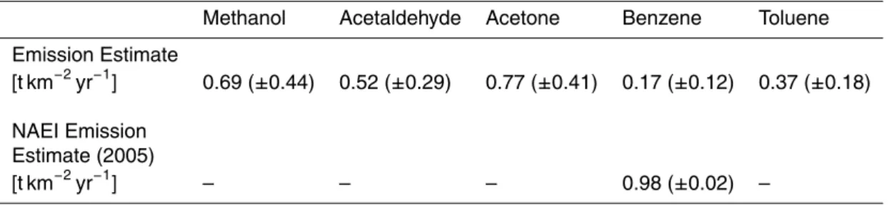
lower, between 19–42µg m−2h−1. The observed fluxes of benzene were up-scaled to give a city wide emission estimate which was found to be significantly lower than that of the National Atmospheric Emissions Inventory (NAEI).

1 Introduction

The compilation of spatially and temporally detailed inventories for the emission of

20

anthropogenic volatile organic compounds (VOCs) from urban areas is a necessary requirement for air quality regulatory purposes, effects assessment and research. Cur-rent emission estimates are associated with large degrees of uncertainty (Friedrich and Obermeier, 1999) which may limit their usefulness. Much of this uncertainty can be attributed to the large variety of different source categories which contribute to

ur-25

(4)

ACPD

8, 245–284, 2008

Full Screen / Esc

Printer-friendly Version Interactive Discussion taking a “bottom-up” inventory approach, an alternative is to make direct

micrometeo-rologically based measurements which can integrate observations of wind speed and scalar concentrations to give a city-wide flux estimate of pollutant emissions (Nemitz et al., 2002; Dorsey et al., 2002; Velasco et al., 2005).

Currently, the eddy covariance (EC) technique is considered the most direct

microm-5

eteorological method available for estimating surface / atmosphere exchange fluxes, as it measures the turbulent flux directly, without reliance on any empirical parameter-isations. This approach requires high frequency measurements (typically in the order of 5–20 Hz) of both vertical wind speed and concentration to resolve all eddies that contribute to vertical transport (Lenschow, 1995). Although this technique is now well

10

established for the measurement of some trace gases, such as CO₂and H₂O (Aubinet et al., 2001), its application to VOC fluxes has been restricted because of the slow response times of most VOC sensors.

A number of alternative micrometeorological approaches have been developed which relax the demands placed upon instrument response times. The technique

15

most commonly applied to VOCs is the relaxed eddy accumulation method (REA), a conditional sampling technique where samples of air are directed into an up or down draught reservoir according to the sign of the vertical wind velocity at the time of sam-pling (Businger and Oncley, 1990). Air from each reservoir is subsequently analysed off-line and a flux is calculated from the difference in concentration generated between

20

the two reservoirs. Unlike the eddy covariance method, REA is not a direct measure of the flux as it relies on empirical parameterisation. Furthermore, there is no scope for retrospective corrections to the coordinate frame (Bowling et al., 1998). Despite these drawbacks, the REA method has been successfully applied to a range of vegetation types including grass land (Olofsson et al., 2003) and forests (Greenberg et al., 2003;

25

Ciccioli et al., 2003; Friedrichs et al., 1999).

More recently a second technique, disjunct eddy covariance (DEC), has been de-veloped for “relaxed” flux measurement. Rather than measuring at high frequencies as in EC, in DEC the flux is calculated using a sub-set of a continuous time series. In

(5)

ACPD

8, 245–284, 2008

Full Screen / Esc

EGU

order to retain the flux contributions carried by small scale eddies, DEC utilises near instantaneous grab samples of air which are aspirated into a storage reservoir at reg-ular intervals. The “dead” time between the sampling periods is then used to analyse the air at a rate suitable for the gas analyser. Provided the interval between samples is kept to less than the integral time scale, then the discontinuous dataset can be used

5

to give high precision flux information, which is numerically similar to the EC approach, but with reduced statistics (Grabmer et al., 2006). The DEC approach is particularly useful for sensors with a response time of 1 to 20 s.

With the advent of quadrupole mass spectrometers (QMS) for the use of atmospheric composition measurements, a range of analysers is now becoming available that can

10

provide fast measurements (as determined by the dwell time on a givenm/z), which is

nevertheless discontinuous (as the QMS scans through a range ofm/z’s). One such

instrument is the proton transfer reaction-mass spectrometer (PTR-MS) which allows for the measurement of most VOCs with good sensitivity (10 ppt) and fast response times (10 Hz).

15

The quadrupole mass spectrometer in the PTR-MS can be programmed to scan over a small suite of masses in what is termed a duty cycle. Although in theory the instrument has a sufficient response time to be compatible with the eddy covariance method, in reality the quadrapole can only scan one mass at a time; therefore the data set returned on completion of each duty cycle is in effect disjunct.

20

To optimise flux measurement approaches for these kind of data, the DEC concept has been developed further to calculate fluxes from the discontinuous time-series at each m/z by pairing up each concentration measurement with the associated wind

measurement in software, a process known as virtual disjunct eddy covariance (vDEC) (Karl et al., 2001, 2002; Spirig et al., 2005; Lee et al., 2006; Ammann et al., 2006;

25

Brunner et al., 2007). The advantage of this technique is that air can be sampled directly into the instrument, as individual masses are measured at a sufficiently fast rate, therefore no additional sampling system is required. Furthermore, analysis times are shorter than in DEC, allowing more data to be collected during each averaging

(6)

ACPD

8, 245–284, 2008

Full Screen / Esc

Printer-friendly Version Interactive Discussion period; consequently the resultant flux estimates are statistically more robust.

The vDEC method has been successfully applied to give VOC flux estimates over vegetation canopies, including grassland (Karl et al., 2001; Ammann et al., 2006; Brun-ner et al., 2007), forests (Karl et al., 2002; Spirig et al., 2005; Lee et al., 2006), and over an urban environment (Velasco et al., 2005).

5

In the current study we deployed both the DEC and vDEC techniques for the mea-surement of a range of VOCs above the city of Manchester (UK). The recorded data were then used to calculate a city-wide emission flux, and in the case of benzene this was compared to the UK National Atmospheric Emission Inventory (NAEI) for Manch-ester (http://www.naei.org.uk/datachunk.php?f datachunk id=174).

10

The NAEI is compiled using a bottom-up approach, where combinations of reported and estimated emissions across numerous source sectors are used to provide a spa-tially disaggregated (1×1 km) emission inventory. The uncertainty associated with these estimates is dependant on the ratio of reported to estimated (modelled) data and hence for compounds such as VOCs, where reported emissions are limited and

15

uncertainty levels are high, micrometeorological methods offer a useful alternative.

2 Methods

2.1 Measurement site and general setup

The work presented here formed part of the UK CityFlux project, which aimed to (i) directly measure pollutant emissions from urban areas, (ii) investigate controls of these

20

emissions, (iii) derive emission factors relative to CO2 and CO and (iv) study

pollu-tant transformation by comparing fluxes at the plume, street canyon and urban canopy scale. During the summer of 2006, micrometeorological measurements of VOC emis-sions were made over the city of Manchester, together with measurements of fluxes and concentrations of VOCs, aerosols, O₃, CO₂and H₂O, as well as mobile

measure-25

(7)

ACPD

8, 245–284, 2008

Full Screen / Esc

EGU

aircraft-borne measurements. The VOC flux measurements were taken from the roof of Portland Tower (53◦28′41′′N; 2◦14′18′′W), an 80 m tall office block, which is located in central Manchester. The building is situated on Portland Street, which is approximately 600 m distance from the Arndale centre, (the city’s principal shopping district) 475 m from Piccadilly railway station, (the north-west’s busiest station), and 100 m from China

5

Town (a concentrated area of restaurants). The building is surrounded by trafficked streets on three sides and a multi-storey car park on the other.

The roof of Portland Tower is not uniformly flat but has three levels. On the lowest level a small shed was erected which housed the PTR-MS. The second level, 2 m above, contained a utility substation which was used to house the sonic anemometer

10

signal box. The roof of the substation was used as the foundation for a 15 m mast which was fitted with a sonic anemometer (Solent Research R3, Gill Instruments Ltd, Lymington, Hants, UK) and Teflon gas inlet line (1/2” OD). The mast was erected to get above the wake effects generated from both the edges of the building and the inhomogeneous roof surface and increased the effective measurement height to 95 m

15

above street level.

Fluxes were measured between the 5 and 20 June 2006. During the first few days of measurements (5th–10th) a high pressure system was centred over Northern Ireland which dominated the weather during this period, with mostly dry conditions, clear skies and temperatures between 16–30◦C. Between the 13th–16th a cold front slowly moved

20

across southern England and during this time temperatures at the measurement tower dropped to a maximum of 24◦C and a minimum of 14◦C on the 16th. For the later part of the campaign, temperatures slowly increased as a high pressure ridge moved in behind the cold front, increasing the average temperature to 21◦C. Throughout the campaign the wind direction shifted between SW and NNE, but also came from the

25

SEE at certain times. The wind speed ranged between 0.4 and 11.2 m s−1, with an average of 3.3 m s−1

(8)

ACPD

8, 245–284, 2008

Full Screen / Esc

Printer-friendly Version Interactive Discussion 2.2 The proton transfer reaction mass spectrometer (PTR-MS)

A standard PTR-MS instrument (Ionicon Analytik, Austria) was used for the measure-ment of VOC concentrations as it offered the desired sensitivity and response times required for both flux systems. Detailed descriptions of this instrument can be found elsewhere (Lindinger et al., 1998; Hayward et al., 2003; de Gouw and Warneke, 2007),

5

therefore only a brief account of the instrument setup will be given here.

The PTR-MS was optimised to an E/N ratio of 125 Td and programmed to sequen-tially scan a suite of six protonated target compounds: methanol (m/z 33),

acetalde-hyde (m/z 45), acetone (m/z 59), isoprene/furan (m/z 69), benzene (m/z 79) and

toluene (m/z 93). In addition to these compounds, the H3O+ primary ion count and 10

two reagent cluster ions were also recorded atm/z 21, m/z 39 and m/z 55,

respec-tively. A further mass,m/z 25, was used at the start of each measurement cycle as a

spacer to ensure the monitored air did not contain residues from the previous sample. The mass detection system of the PTR-MS can only record VOC (ion counts per second) in atomic mass units (amu); therefore it is difficult to attribute ion counts to

in-15

dividual VOC species. Interference from other ions at amu 33, 45, 79 and 93 has been shown to be insignificant in previous studies (de Gouw et al., 2007), but both acetone and propanal have been detected at amu 59. Although this can generate some un-certainty in the measurement of acetone, the signal of acetone is always dominant in ambient air (Kato et al., 2004), therefore ion counts recorded atm/z 59 were ascribed 20

solely to acetone in the present study. Similarly m/z 69 may be isoprene and/or

fu-ran, although the latter is normally present at very low concentrations in ambient air (Christian et al., 2004). Massm/z 69 was therefore solely attributed to isoprene.

The VOC concentrations were calculated using reaction rate constants (k) from Zaho

and Zhang (2004) and transmission numbers (the time taken for each mass to traverse

25

the drift tube) calculated usingt=L/vd, whereL is the length of the drift tube and vd is

(9)

ACPD

8, 245–284, 2008

Full Screen / Esc

EGU

2.3 Flux measurements

During the campaign, two flux measurement techniques (DEC and vDEC) were em-ployed to measure surface layer fluxes of VOCs from the urban canopy. As both tech-niques utilised a single PTR-MS instrument to give VOC concentrations, it was not possible to operate the systems simultaneously, and therefore fluxes were measured

5

by the two methods in alternate half hours. A Teflon 3-way solenoid valve (001-0017-900, Parker Hannifin) sat in line and enabled the PTR-MS to switch freely between the two systems. Flux measurements in each mode were averaged over a 25 min period and the remaining 5 min of each half hour were used to scan the entire mass spec-trum (m/z 21–146) to give basic ambient concentration information on a wide range of 10

VOCs. Figure 1 shows a typical PTR-MS operating sequence during 1 h of measure-ments and includes the PTR-MS duty cycles for each flux mode.

2.3.1 Virtual disjunct eddy covariance sampling system (vDEC)

During the first period of each hour, the 3-way solenoid valve was triggered to enable the PTR-MS to sub-sample directly from the main sample line in a virtual disjunct eddy

15

covariance mode. The quadrapole was set to scan each mass at a rate of 20 ms, allowing sample air to be purged directly into the instrument without the use of an additional sampling system. The inlet for the sample line was mounted a short distance below the sonic anemometer, as vertical displacement has been shown to result in the smallest flux losses (Kristensen et al., 1997). In order to maintain a turbulent flow

20

through the sample line, and thus avoid dampening of the VOC signal, a flow rate of 60 l min−1 was used. Upon the completion of each PTR-MS duty cycle, data were exported to a LabVIEW logging programme using the Microsoft Windows “dynamic data exchange” (DDE) protocol, which stored the data alongside those from the sonic anemometer.

(10)

ACPD

8, 245–284, 2008

Full Screen / Esc

Printer-friendly Version Interactive Discussion 2.3.2 Disjunct flux sampling system (DFS)

A disjunct flux sampling system was deployed on the roof of the building to monitor the VOC fluxes for the second period of each hour. The schematic and operating sequence of the DFS are depicted in Fig. 2. The sampler comprised two one litre stainless steel canisters, which act as intermediate storage reservoirs (ISR) for sampled air.

5

Fast switching high flow conductance valves (Lucifer E121K45) were mounted to the inlet of each canister, enabling the ISR to take a fast grab sample once activated. Each ISR was coiled with heater cable and insulated with aluminium foil to maintain an internal temperature of 40◦C. This, combined with the cylindrical shape of the canisters which reduced surface area, helped to minimise losses of VOC to walls, and minimised

10

condensation and the formation of liquid water, which can remove soluble compounds such as methanol.

Before grab samples of air were taken, each ISR was first evacuated to a pressure of 250 mbar. The time taken to evacuate the canister, 12 s, was the limiting factor in determining the length of time between sampling. By contrast, the time taken to fully

15

pressurise the ISRs, 0.5 s, proved to be the limiting factor in determining sampling times. Therefore the overall effective response time of the DFS setup is about 0.5 s, which is sufficient to resolve turbulent fluctuations of up to 2 Hz.

Grab samples of air acquired by the DFS were analysed for VOCs using the PTR-MS, which was connected to the DFS via a 4 m length of 1/8” PFA tubing. The rate

20

at which the PTR-MS draws air from the ISR is important as a vacuum is gradually generated as air is sampled. This back-pressure can affect the pressure in the drift tube, which can lead to small changes in theE/N ratio of the instrument. In order to

prevent this problem, the flow rate of the PTR-MS was reduced from 300 ml min−1 to 150 ml min−1.

25

The PTR-MS was housed some distance from the sonic anemometer. Thus the sampling line between ISRs and PTR-MS would have been too long for the DFS to be mounted on the anemometer mast. Instead it was located at the base of the tower,

(11)

ACPD

8, 245–284, 2008

Full Screen / Esc

EGU

with each sample valve connected via a “T-piece” into the1_/₂_{” OD sampling line. As a}

drawback of this setup, the sample line is subject to a pressure drop of approximately 200 mbar, caused by the high flow rates used. Consequently, upon activation of sam-ple valves each ISR could only pressurise to 800 mbar, increasing their effective carry-over between samples from 25% under normal operating conditions (at 1000 mbar) to

5

∼31%. The carryover was corrected using the following equation:

χcor= (χ × P1−χold×P2)/(P1−P2) (1)

whereχ is the VOC concentration within the ISR, χold is the previous concentration

of the same ISR,P1 is the ISR pressure when full and P2 is the ISR pressure after

evacuation.

10

The sequence of valve switching used to control both the sample and analysis phases of the DFS, which combined with valve switching, pressure recording, sonic anemometer and PTR-MS data recording, were all coordinated using LabVIEW soft-ware (National Instruments – v 6.1). The valves were controlled through a multifunction IO card (6071E, National Instruments), which also recorded the analogue signals from

15

the pressure sensors of the ISR (OMEGA, Stamford, Connecticut, PX137-015DV). 2.3.3 Flux calculations

In the eddy covariance technique, the flux of an atmospheric scalar is calculated using the covariance between continuous time series of vertical wind speed and scalar con-centration at a fixed point in space over a statistically representative time period. Since

20

the data generated by the disjunct flux systems are simply a sub-set of the continuous time series, the flux may be calculated in the same way; thus observations of vertical wind velocity (w) were paired with the corresponding PTR-MS data (χ ) to give a flux

as follows:

F χlag = w′χ′ (2)

(12)

ACPD

8, 245–284, 2008

Full Screen / Esc

Printer-friendly Version Interactive Discussion where primes indicate instantaneous fluctuations about the mean and over-bars

de-note time averaging (i.e.w′=w − w). The only difference between this and direct eddy covariance measurements is the reduced number of data points used for the flux cal-culation, which results in an increase in the statistical uncertainty of the measurement. Before the flux can be calculated it is first necessary to correct for the time lag that

5

exists between the two data sets, which occurs because of the ∼25 m separation be-tween the sonic anemometer and the PTR-MS. This time lag was calculated from the maximum value in a cross correlation function betweenw and χ within a 5 s time

win-dow. This value was then used to realign the time series ofw′andχ′and calculate the flux. Typically the peak in the cross correlation was noted between 3 and 5 s, which

10

compared closely with the theoretically calculated lag time of ∼3 s.

Standard rotations of the coordinate frame were applied to correct for tilting of the sonic anemometer. The vertical rotation angle showed a clear relationship with wind direction, with maximum values of up to 15◦. This is similar to other flux measure-ments in the urban environment (e.g. Nemitz et al., 2002) and suggests that, although

15

the mean airflow at the anemometer is affected by the building, the influence can be compensated by standard rotational corrections.

Calculated fluxes were subject to a post-processing algorithm which filtered and re-moved data that failed to meet specified quality controls. These included removal of large spikes in vertical wind speed or VOC concentration and the omission of data

20

where the average wind speed dropped below 1 m s−1. This latter QA procedure re-sulted in the loss of 7% of the flux data.

In addition, during post-processing of the data, it was found that the inlet pump was occasionally shut down by its thermal trip. The affected time periods were filtered and the spikes removed, affected averaging periods were not included in the final flux

25

analysis. This meant approximately 31% of measured flux data was deemed unusable and are not shown here.

(13)

ACPD

8, 245–284, 2008

Full Screen / Esc

EGU

3 Results and discussion

3.1 VOC concentrations

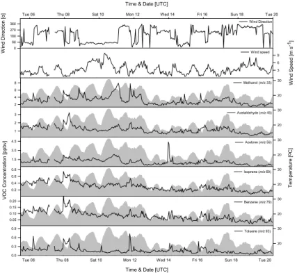
Concentrations of VOCs are summarised in Table 1 and the 25 min average values are plotted alongside temperature and wind direction in Fig. 3. The oxygenated com-pounds, methanol, acetone and acetaldehyde, were the most abundant (methanol 1.3–

5

8 ppbv; acetone 0.3–4.4 ppbv; acetaldehyde 0.44–3.2 ppbv). The larger concentrations of methanol compared with the other analytes are typical for urban VOC measurements and can be attributed to its relatively low photochemical reactivity (Atkinson, 2000) and the numerous anthropogenic/biogenic sources which contribute to its emissions both in and outside of the city (de Gouw et al., 2003). Comparisons of methanol

concen-10

trations with previous studies shows the values observed here to be within the lower range of concentrations measured in Barcelona (Filella and Penuelas, 2006) and within the range of values recorded in Innsbruck (Holzinger et al., 2001). The concentrations of the other two oxygenated compounds, acetone and acetaldehyde, both lie within the range of data reported from other major conurbations such as Rome (Possanzini et al.,

15

1996), Los Angeles (Grosjean et al., 1996) and Rio de Janiero (Grosjean et al., 2002). Concentrations of isoprene ranged between 0.07–0.75 ppbv, which is consistent with values obtained from the national air quality monitoring network (http://www.airquality.

co.uk/archive/reports/cat13/0602011042 q3 2005 rat rep issue1 v5.pdf) for other UK cities, including Bristol and London. The aromatic compounds, benzene and toluene,

20

were the least abundant of the VOCs measured, ranging between 0.02–0.2 and 0.03– 0.73 ppbv, respectively. These values also compared well with data obtained from the National network (www.airquality.co.uk) automatic monitoring station on Marylebone Road, London, although, on average, concentrations from the London site were higher, presumably due to the kerbside location of the sampler, compared with a sampling

25

height of 95 m for the concentrations reported here.

Strong linear relationships were observed between the concentrations of each of the measured VOCs, with R2 values ranging between 0.24 and 0.85, suggesting some

(14)

ACPD

8, 245–284, 2008

Full Screen / Esc

Printer-friendly Version Interactive Discussion commonality between the sources of emission for each of the compounds.

Clear day-night trends in mixing-ratios were not apparent, with maxima occasionally observed at night time (Thursday 8th, Saturday 11th), whereas on other days (Satur-day 17th–Tues(Satur-day 20th) they tended to peak during the late afternoon. Spikes were frequently observed in the concentration of methanol during the early morning. This

5

often corresponded to low temperatures and low wind speed in the early morning and is consistent with previous urban VOC studies which have attributed this increase to condensation processes (Fiella and Penuelas, 2006). The nocturnal increase in con-centrations for the other compounds is unclear, but is likely a combination of small night-time emissions accumulating in the shallow nocturnal boundary layer, the

dy-10

namics of which differed between the different nights. These emissions may include combustion and fugitive emissions from industrial activity outside the flux footprint, on the outskirts of the city.

Additional spikes in VOC concentrations can be observed in Fig. 3. While some of these can be ascribed to changes in wind direction, such as those observed inm/z 59 15

on the 14th, others, as seen inm/z 93 on the 16th cannot.

Figure 4 shows scatter plots of VOC mixing ratios measured during the vDEC mode between the 5 and 20 June. These plots are useful for the interpretation and source ap-portionment of data. For example, strong linear relationships, as seen in panel (I), may suggest a similar source contributing to the emission of the two compounds, whereas

20

in panel (K), where a bimodal distribution is evident, it is possible that there are two separate sources contributing to the observed VOC concentrations. Further informa-tion can be obtained from these plots by differentiating data points by a z axis, in this case temperature, which in some instances (panel (E)) can reveal what appears to be a temperature dependency in the measured concentration of the VOC. To help with

25

the further interpretation of the data shown in Fig. 4, Table 2 lists some of the known anthropogenic, biogenic and chemical sources of the measured compounds and also includes atmospheric lifetimes with respect to OH, NO3, O3and photolysis.

(15)

ACPD

8, 245–284, 2008

Full Screen / Esc

EGU

(m/z 79). Both these compounds are known constituents of petrol fuel (Borbon et al.,

2001), and consequently they are emitted to the atmosphere by the same two anthro-pogenic sources: direct emissions from vehicle exhausts and evaporative emissions from petroleum products, hence the strong linear relationship (R2=0.87 (p<0.0001)) observed between the two compounds during this study. Despite the apparent clarity

5

of this relationship, more detailed analysis of the data with respect to temperature, as shown in Fig. 5, indicates the observed isoprene concentrations to be strongly influ-enced by the ambient air temperature, with higher concentrations relative to those of benzene observed during warmer conditions. It is reasonable to presume that the com-position of vehicle exhaust is unlikely to vary significantly with changes in the observed

10

ambient air temperature (16–30◦C), therefore it must be assumed that this increase occurs either due to increased evaporative emissions, as isoprene is more volatile than benzene, or that there are emissions of isoprene from a third source, indepen-dent of that of benzene. Biogenic emissions of isoprene are an obvious candidate, as isoprene emission rates from plants have been shown to be both temperature and

15

light dependant (Guenther et al., 1995). Yet, analysis of an isoprene inventory for Great Britain (Stewart et al., 2003) shows few biogenic sources of isoprene within the city centre. Analysis of the meteorology during the period, when the ambient air temperature was at its highest, shows the average wind speed to be approximately 8 m s−1. Although isoprene has a short atmospheric lifetime in the daytime, typically

20

on the order of 1 h (Atkinson, 2000), due to reactions with the OH radical, at such wind speeds, air masses containing isoprene emitted from rural areas, outside of the city could have reached the tower before removal by OH. Consequently it is assumed that the temperature-dependent fraction of isoprene observed during this study was a com-bination of both evaporative and biogenic emissions. The percentage contribution of

25

temperature-dependent isoprene is shown in Fig. 6. This plot suggests that at 30◦C as much as 32% of the observed isoprene within the city centre could be due to a combination of evaporative and biogenic emissions. Separation of these two sources to obtain the biogenic fraction is not possible.

(16)

ACPD

8, 245–284, 2008

Full Screen / Esc

Printer-friendly Version Interactive Discussion Toluene was the least volatile of the compounds measured during this study and the

ratios of its concentration against those of benzene, isoprene, acetone, acetaldehyde and methanol did not vary with temperature (Fig. 4: panels (B), (C), (E), (H) and (K), respectively). However, in each of these plots, bimodal distributions were observed and each of the aforementioned compounds appeared to demonstrate some degree of

5

temperature dependency with respect to toluene, although this varied between com-pounds. Acetone appearing to be highly temperature dependant, whereas benzene showed only a slight variation with temperature. In the case of benzene, the observed temperature dependence may be coincidental and due to the prevailing wind direction and increased wind speeds which accompanied the elevated temperatures. This point

10

can be highlighted by investigation of the ratio of benzene to toluene concentrations in Fig. 7. As both of these compounds are known to be present in primary vehicle exhaust emissions (Jobson et al., 2005), and have differing atmospheric lifetimes with respect to the OH radical, analysis of the benzene to toluene ratio (B/T) can be used to gauge the age of an air mass (Warneke et al., 2001). Previous studies have shown the

15

B/T ratio in primary exhaust emissions to typically lie in the range of 0.41–0.83 (Heeb et al., 2000), but this ratio increases as toluene reacts with the OH radical faster than benzene and is preferentially removed over time in the atmosphere. In the present study the average B/T ratio was approximately 0.55 (Fig. 7), suggesting the observed concentrations were typically originating from sources close to the measurement site.

20

However, during the period of elevated temperatures (9–12 June), the ratio increased to approximately 0.67, which suggests slightly older, photochemically processed, air was being advected from outside of the city. In the days before this period (6–9 June), the wind direction was from the SW. As the temperatures increased between the 9th and 12th, the wind direction rotated 180◦and the air that had left the city in the days

pre-25

viously was transported back across Manchester. The atmospheric lifetime of toluene with respect to OH is approximately 2 days (Atkinson, 2000), which corresponds to an advection distance of ∼1300 km under the prevailing average wind speed. Taking this into account, the returning air mass would be depleted in toluene and therefore the

(17)

ACPD

8, 245–284, 2008

Full Screen / Esc

EGU

ratio of benzene to toluene in the air mass would increase, which can be seen occur-ring in Fig. 7. In addition, the removal rate of toluene may have been increased due to higher concentrations of the OH radical corresponding to the increase in temperature. Therefore it can be concluded that, although some temperature dependency may be observed due to increased evaporative emissions and OH concentrations, the bimodal

5

distributions observed in Fig. 4 panels (B), (C), (E), (H) and (K) are, in part, a result of an older air mass being advected back across the city, in which the toluene has been removed through reaction with the OH radical. Fig. 7 also demonstrates the diurnal cycle in the B/T ratio due to changes of OH concentrations over the day.

Acetone (m/z 59) appeared to show the greatest degree of temperature depen-10

dence out of all the measured VOCs. Like acetaldehyde, acetone can be formed in the atmosphere as a product of the photooxidation of hydrocarbons, including propane, isobutene and isopentane (Singh and Zimmerman, 1992). These are primary vehicle exhaust pollutants (Hwa, 2002; Chiang et al., 2007); however, the atmospheric lifetime of each is typically on the order of tens of days, therefore temperature-dependant

pho-15

tooxidation is unlikely to be a major source of acetone within the city. Both acetone and acetaldehyde are themselves found in vehicle exhaust emissions (Sigsby et al., 1987; Caplain et al., 2006), which accounts for the close relationship observed with benzene concentrations. Again, the apparent temperature dependency of these com-pounds, seen in Fig. 4 panels (D) and (G), could be related to the high volatilities of

20

these compounds, leading to fugitive evaporative emissions at higher temperatures. Al-though acetaldehyde is more volatile than acetone, and therefore should demonstrate the greatest tendency to evaporate at higher temperatures, acetone has a wider distri-bution of potential sources as it is not only found in petrol but also in a wide range of solvents and cleaning fluids (Table 2).

25

3.2 VOC fluxes

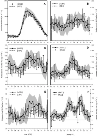
Averaged diurnal fluxes for the period 5–20 June 2006, as measured by both the DEC and vDEC techniques, are shown in Fig. 8. Despite some variability between the two

(18)

ACPD

8, 245–284, 2008

Full Screen / Esc

Printer-friendly Version Interactive Discussion systems, both techniques show VOC fluxes to have a clear diurnal trend, with fluxes at

their largest in the mid to late afternoon and lowest in the early hours of the morning. On average, fluxes were positive for most of the day, indicating the city to be acting as a net source of VOC to the atmosphere, although deposition was observed for short periods in the night. Typically, emissions rose sharply just after sunrise between

5

06.00 and 10.00 h, peaking at around midday for most compounds. This morning rise coincided with the peak in traffic counts which were taken on Oxford Road, a busy street adjacent to Portland Street, which provides a good proxy of the relative change of the diurnal traffic pattern in the area.

On average, fluxes of acetone were the largest (88µg m−2h−1) followed by methanol,

10

(79µg m−2h−1) and acetaldehyde, (60µg m−2h−1), whereas fluxes of the aromatic compounds benzene and toluene were lower (19µg m−2h−1 and 42µg m−2h−1, re-spectively). Isoprene fluxes were omitted from the final analysis, as significant dif-ferences were observed between the two techniques, indicating a possible source of contamination in one or other of the systems.

15

Panel B, Fig. 9, shows the average daily flux of methanol. Typically, fluxes of methanol started to increase at around 08:00, rising steadily until an early evening maximum between 17:00 and 19:00 h. At this time fluxes dropped off sharply before levelling and reaching a minimum during the early morning.

Panel C shows the flux of acetaldehyde, which tended to have two afternoon maxima,

20

the first and largest at around 13:00 h, and the second coinciding with that of methanol at 19:00 h. Similarly, both benzene (panel E) and toluene (panel F) demonstrated a two peak trend. In the case of benzene, the first peak, which occurred typically around 13:00 h was higher than the second, which occurred at 19:00 h. For toluene the reverse was true, with the second peak, again occurring at 19:00 h, being larger than the first

25

at 11:00 h. Acetone (panel D) did not follow the same pattern of emission; instead, it demonstrated a clear single peak (13:00 h) which was not dissimilar to that of the sensible heat flux shown in panel A. Unlike the other compounds, acetone had no peak at around 19:00 h, which may suggest a shift in emission sources at this time.

(19)

ACPD

8, 245–284, 2008

Full Screen / Esc

EGU

These diurnal trends suggest that toluene, benzene and acetaldehyde are primarily derived from direct traffic emissions as they follow the traffic pattern most closely. Ace-tone shows a different pattern which may be due to emission from other anthropogenic activities such as solvent use. Methanol emissions are broader over the day, consis-tent with a large contribution from fugitive sources that are coupled to a combination of

5

temperature and anthropogenic activity.

Despite the indirect nature of this comparison, the two flux measurement systems showed reasonable agreement, with measured fluxes falling within the range of the calculated uncertainty (standard error of hourly fluxes). The highest observed correla-tions between the DEC and vDEC techniques were observed in the fluxes of toluene

10

and acetone, which hadR2 values of 0.79 (_{p<0.0001; N=48) and 0.72 (p<0.0001),} respectively. Methanol (R2=0.2 p<0.0288) and acetaldehyde (R2=0.45 p<0.0003) compared less well, as did benzene (R20.36 p< 0.0001), which, during the mid to

late afternoon showed discrepancies between the two techniques. During this time the DEC system underestimated fluxes measured by the vDEC technique in a trend that

15

was noticeable in all measured fluxes with the exception of methanol.

On average fluxes recorded by the vDEC system were 19% (absolute error) larger than those measured by the DEC system, although this value varied significantly be-tween the individual masses, with no observed underestimation for methanol and ap-proximately 40% underestimation for benzene. The most likely cause of this

discrep-20

ancy is the difference in the effective response times of the two systems, as the vDEC system was able to resolve turbulent fluctuations of up to 20 Hz as opposed to 2 Hz for the DEC system. The slower sampling resolution of the DEC system meant high frequency flux contributions may have been attenuated and lost and therefore the total flux was underestimated.

25

The portion of the flux attenuated by the slower measurement resolution can be es-timated theoretically using wind and temperature data [20 Hz] to calculate the sensible heat flux. Extracting data points to correspond with the activation of DEC sampling valves generates a disjunct time series which can be compared to the original EC

(20)

ACPD

8, 245–284, 2008

Full Screen / Esc

Printer-friendly Version Interactive Discussion sensible heat flux. Reducing the effective sampling times of the data from 0.05 s to

0.5 s is achieved by simply extracting ten temperature measurements instead of one and using the average value for the flux calculation. When this technique was ap-plied to the sensible heat data (Fig. 9, panel A), the simulated DEC fluxes typically underestimated the EC fluxes by approximately 8%. This suggests that some of the

5

underestimation observed between the two systems is caused by the slower resolution of the DEC system but not all; therefore there are other sources of error which have yet to be quantified. One possible explanation is that the sampling response of the DFS is<2 Hz, possibly because of adsorption / desorption effects in the ISRs for more

“sticky” compounds. In addition, the differences between the two techniques seemed to

10

be inversely proportional to VOC concentrations, hence benzene, which was the least abundant compound measured, demonstrated the largest deviation between the two data sets. This suggests the measurements of benzene were close to the detection limit of the instrument. In future this could be improved by increasing the integration time of the vDEC measurement from a dwell time of 20 ms to 0.1 or 0.2 s.

15

3.3 Comparison of measured benzene fluxes with NAEI estimates

Measured fluxes of benzene were up-scaled and compared against the most recent (2005) emission estimate for Manchester taken from the National Atmospheric Emis-sion Inventory (http://www.naei.org.uk/datachunk.php?f datachunk id=174). The flux estimates from the vDEC system were used for the comparison as they did not

suf-20

fer from the attenuation of high frequency flux contributions. In order to compare the up-scaled fluxes with the inventory it was first necessary to calculate the flux foot print (surface area contributing to the flux) so that the appropriate NAEI grid(s) could be selected for comparison.

Footprints were calculated using a simple parameterisation model developed by

25

Kljun et al. (2004) which was run using typical urban meteorology to give footprints under stable, neutral and convectively unstable atmospheric conditions. This model is designed for dynamically homogenous terrain, therefore its application to the urban

(21)

ACPD

8, 245–284, 2008

Full Screen / Esc

EGU

environment is not ideal; however there are few if any operational footprint models de-signed for this type of environment. Therefore the flux footprints obtained are treated as a first-order estimate only. The following parameters were used in the model: stan-dard deviation of vertical wind velocity σ_w=0.3 m s−1; friction velocity u∗=0.3 m s−1; measurement heightzm=95 m; roughness length z0=0.4 m; and boundary layer height 5

h=250 m (stable), 1000 m (neutral) and 2000 m (unstable). The results are shown in

Fig. 9 and list the distance at which the maximum contribution to the flux can be ex-pected (X_max) and the distance at which 80% of the flux is contained (X_r).

In order to calculate an emission estimate for the city using these data, it was as-sumed that the observed average fluxes were representative of the benzene

emis-10

sion rates occurring throughout the year (although the emission rates of benzene are likely to show some seasonal variation, with increased vehicle use during the winter months causing higher direct emissions, this may be balanced by the increased fugi-tive emissions in the summer months). Therefore the measured average total daily flux of benzene (454µg m−2d−1) was extrapolated to give an annual emission estimate of

15

0.17 (±0.12) t km−2yr−1. This value is six times lower than that predicted by the NAEI (0.98 t km−2yr−1) for Manchester city centre in 2005.

Since the implementation of both the Geneva VOC (UN ECE, 1991) and the Gothen-burg multi-pollutant Protocols (UN ECE, 1999) annual average mean benzene concen-trations have declined in the UK at a rate of approximately −20% per year (Dollard et

20

al., 2007). This decrease has been brought about largely through the implementation of three way catalysts to control vehicle emissions and the use of canisters to control the evaporative emissions. Taking this decline into consideration and readjusting the 2005 NAEI emission estimate accordingly, a revised emission estimate of 0.78 t km−2yr−1 for 2006 is realised. However this figure is still significantly higher than the measured

25

fluxes. Reasons for this large discrepancy are uncertain, but are likely to involve either poorly characterised VOC sources and/or activity statistics within the NAEI, or, a sta-tistically unrepresentative measurement of benzene fluxes by the vDEC technique, or a combination of both.

(22)

ACPD

8, 245–284, 2008

Full Screen / Esc

Printer-friendly Version Interactive Discussion Measured flux estimates for the remaining five compounds are shown in Table 3,

but the NAEI does not explicitly estimate their emission rates, so further comparisons were not possible. Published VOC fluxes from the urban environment are limited, but fluxes have been measured above Mexico City using a vDEC approach as part of the Mexico City Metropolitan Area 2003 field campaign. Average fluxes of methanol

5

(1044µg m−2h−1), toluene (828µg m−2h−1) and acetone (396µg m−2h−1) were found between four and nineteen times higher than those observed in Manchester. This is unsurprising given the much older vehicle fleet, less dominance of catalytic converters and poorer fuel quality in Mexico City, where vehicle emissions are not regulated by the aforementioned protocols.

10

4 Conclusions

In the past the virtual and disjunct eddy covariance techniques have been successfully applied to give flux information from a range of vegetation canopies. In the present study we have shown that these techniques can be extended to the urban environment provided a measurement site with suitable elevation above street level can be found.

15

We have also demonstrated the effectiveness and limitations of each approach. The vDEC technique is thought to be more suited for urban flux work due to its relative simplicity and fast response time. However, the DEC technique has also been shown to be effective and, with improvements to the system design, such as increased mea-surement frequency and tower mounting capabilities, could become an important tool

20

in increasing our understanding of both anthropogenic and biogenic VOC emissions. Emission estimates derived using flux data from the vDEC technique demonstrate the potential of using VOC flux measurements in determining emission estimates on a city wide scale. Although emission estimates obtained in this study are based on a “snap shot” of the total yearly emission, they demonstrate the potential of the technique,

25

which, if deployed on a longer time scale such as a year could give very detailed information on urban-scale emissions, including both spatial and, more importantly,

(23)

ACPD

8, 245–284, 2008

Full Screen / Esc

EGU

temporal trends, which are currently not accounted for in the NAEI emission estimates. Finally, we have demonstrated that ambient air temperature plays an important role in the relative concentrations of VOCs in urban air. While some compounds are solely governed by their volatility and increased evaporation rates at higher temperatures, others such as isoprene, can also be influenced by increased biogenic emissions

oc-5

curring both in, and outside of the city.

Acknowledgements. We thank Bruntwood Estates Ltd for allowing access to Portland Tower and for the cooperation and support of their staff. The work was funded by the UK Natural Envi-ronmental Research Council through the “CityFlux” grant and an NCAS studentship and by the ESF VOCBAS programme. We thank I. Longley (Manchester University) who was responsible

10

for the organisation and logistics of the campaign, G. Phillips (CEH Edinburgh) for his help transporting the instrumentation and M. Possell (Lancaster University) for helpful discussion.

References

Ammann, C., Brunner, A., Spirig, C., and Neftel, A.: Technical note: Water vapour concentration and flux measurements with PTR-MS, Atmos. Chem. Phys., 6, 4643–4651, 2006,

15

http://www.atmos-chem-phys.net/6/4643/2006/.

Anderson, L. G., Lanning, J. A., Barrell, R., Miyagishima, J., Jones, R. H., and Wolfe, P.: Sources and sinks of formaldehyde and acetaldehyde: An analysis of Denver’s ambient concentration data, Atmos. Environ., 30, 2113–2123, 1996.

Atkinson, R.: Atmospheric chemistry of VOC and NOx, Atmos. Environ., 34, 2063-2101, 2000.

20

Aubinet, M., Chermanne, B., Vandenhaute, M., Longdoz, B., Yernaux, M., and Laitat, E.: Long term carbon dioxide exchange above a mixed forest in the Belgian Ardennes, Agr. Forest Meteorol., 108, 293–315, 2001.

Borbon, A., Fontaine, H., Veillerot, M., Locoge, N., Galloo, J. C., and Guillermo, R.: An inves-tigation into the traffic-related fraction of isoprene at an urban location, Atmos. Environ., 35,

25

3749–3760, 2001.

Bowling, D. R., Turnipseed, A. A., Delany, A. C., Baldocchi, D. D., Greenberg, J. P., and Monson, R. K.: The use of relaxed eddy accumulation to measure biosphere-atmosphere exchange of isoprene and of other biological trace gases, Oecologia, 116, 306–315, 1998.

(24)

ACPD

8, 245–284, 2008

Full Screen / Esc

Printer-friendly Version Interactive Discussion Brunner, A., Ammann, C., Neftel, A., and Spirig, C.: Methanol exchange between grassland

and the atmosphere, Biogeosciences, 4, 395–410, 2007, http://www.biogeosciences.net/4/395/2007/.

Businger, J. A. and Oncley, S. P.: Flux measurement with conditional sampling, J. Atmos. Ocean Tech., 7, 349–352, 1990.

5

Caplain, I., Cazier, F., Nouali, H., Mercier, A., Dechaux, J. C., Nollet, V., Journard, R., Andre, J. M., and Vidon, R.: Emissions of unregulated pollutants from European gasoline and diesel passenger cars, Atmos. Environ., 40, 5954–5966, 2006.

Chiang, H. L., Hwu, C. S., Chen, S. Y., Wu, M. C., Ma, S. Y., and Huang, Y. S.: Emission factors and characteristics of criteria pollutants and volatile organic compounds (VOCs) in a freeway

10

tunnel study, Sci. Total Environ., 381, 200–211, 2007.

Christian, T. J., Kleiss, B., Yokelson, R. J., Holzinger, R., Crutzen, P. J., Hao, W. M., Shirai, T., and Blake, D. R.: Comprehensive laboratory measurements of biomass-burning emissions: 2. First intercomparison of open-path FTIR, PTR-MS, and GC-MS/FID/ECD, J. Geophys. Res.-Atmos., 109, D02311, doi:10.1029/2003JD003874, 2004.

15

Ciccioli, P., Brancaleoni, E., Frattoni, M., Marta, S., Brachetti, A., Vitullo, M., Tirone, G., and Valentini, R.: Relaxed eddy accumulation, a new technique for measuring emission and deposition fluxes of volatile organic compounds by capillary gas chromatography and mass spectrometry, J. Chromatogr. A, 985, 283–296, 2003.

de Gouw, J. and Warneke, C.: Measurements of volatile organic compounds in the Earth’s

20

atmosphere using proton-transfer-reaction mass spectrometry, Mass. Spectrom. Rev., 26, 223–257, 2007.

de Gouw, J., Warneke, C., Karl, T., Eerdekens, G., van der Veen, C., and Fall, R.: Sensitivity and specificity of atmospheric trace gas detection by proton-transfer-reaction mass spectrometry, Int. J. Mass. Spectrom., 223, 365–382, 2003.

25

de Gouw, J. A., Howard, C. J., Custer, T. G., Baker, B. M., and Fall, R.: Proton-transfer chemical-ionization mass spectrometry allows real-time analysis of volatile organic compounds re-leased from cutting and drying of crops, Environ. Sci. Technol., 34, 2640–2648, 2000. Dollard, G. J., Dumitrean, P., Telling, S., Dixon, J., and Derwent, R. G.: Observed trends

in ambient concentrations of C-2-C-8 hydrocarbons in the United Kingdom over the period

30

from 1993 to 2004, Atmos. Environ., 41, 2559–2569, 2007.

Dorsey, J. R., Nemitz, E., Gallagher, M. W., Fowler, D., Williams, P. I., Bower, K. N., and Beswick, K. M.: Direct measurements and parameterisation of aerosol flux, concentration

(25)

ACPD

8, 245–284, 2008

Full Screen / Esc

EGU

and emission velocity above a city, Atmos. Environ., 36, 791–800, 2002.

Filella, I. and Penuelas, J.: Daily, weekly, and seasonal time courses of VOC concentrations in a semi-urban area near Barcelona, Atmos. Environ., 40, 7752–7769, 2006.

Friedrich, R. and Obermeier, A.: Anthropogenic Emissions of Volatile Organic Compounds, Reactive Hydrocarbons in the Atmosphere, Hewitt, C. N. Academic Press, California, 1–39,

5

1999.

Grabmer, W., Graus, M., Lindinger, C., Wisthaler, A., Rappengluck, B., Steinbrecher, R., and Hansel, A.: Disjunct eddy covariance measurements of monoterpene fluxes from a norway spruce forest using PTR-MS, International Journal of Mass Spectrometry, 239, 111–115, 2004.

10

Greenberg, J. P., Guenther, A., Harley, P., Otter, L., Veenendaal, E. M., Hewitt, C. N., James, A. E., and Owen, S. M.: Eddy flux and leaf-level measurements of biogenic VOC emis-sions from mopane woodland of Botswana, J. Geophys. Res.-Atmos., 108(D13), 8466, doi:10.1029/2002JD002317, 2003.

Grosjean, D., Grosjean, E., and Moreira, L. F. R.: Speciated ambient carbonyls in Rio de

15

Janeiro, Brazil, Environ. Sci. Technol., 36, 1389–1395, 2002.

Grosjean, E., Grosjean, D., Fraser, M. P., and Cass, G. R.: Air quality model evaluation data for organics .2. C-1-C-14 carbonyls in Los Angeles air, Environ. Sci. Technol., 30, 2687–2703, 1996.

Guenther, A., Geron, C., Pierce, T., Lamb, B., Harley, P., and Fall, R.: Natural emissions of

non-20

methane volatile organic compounds; carbon monoxide, and oxides of nitrogen from north america, Atmos. Environ., 34, 2205–2230, 2000.

Guenther, A., Hewitt, C. N., Erickson, D., Fall, R., Geron, C., Graedel, T., Harley, P., Klinger, L., Lerdau, M., McKay, W. A., Pierce, T., Scholes, B., Steinbrecher, R., Tallamraju, R., Taylor, J., and Zimmerman, P.: A global model of natural volatile organic-compound emissions, J.

25

Geophys. Res.-Atmos., 100, 8873–8892, 1995.

Hayward, S., Hewitt, C. N., Sartin, J. H., and Owen, S. M.: Performance characteristics and applications of a proton transfer reaction-mass spectrometer for measuring volatile organic compounds in ambient air, Environ. Sci. Technol., 36, 1554–1560, 2002.

Heeb, N. V., Forss, A. M., Bach, C., Reimann, S., Herzog, A., and Jackle, H. W.: A comparison

30

of benzene, toluene and C-2-benzenes mixing ratios in automotive exhaust and in the sub-urban atmosphere during the introduction of catalytic converter technology to the Swiss car fleet, Atmos. Environ., 34, 3103–3116, 2000.

(26)

ACPD

8, 245–284, 2008

Full Screen / Esc

Printer-friendly Version Interactive Discussion Holzinger, R., Jordan, A., Hansel, A., and Lindinger, W.: Methanol measurements in the lower

troposphere near Innsbruck (047◦16′N; 011◦24′E), Austria, Atmos. Environ., 35, 2525–2532, 2001.

Hurst, D. F., Griffith, D. W. T., and Cook, G. D.: Trace gas emissions from biomass burning in tropical Australian savannas, J. Geophys. Res.-Atmos., 99, 16 441–16 456, 1994.

5

Hwa, M. Y., Hsieh, C. C., Wu, T. C., and Chang, L. F. W.: Real-world vehicle emissions and VOCs profile in the Taipei tunnel located at Taiwan Taipei area, Atmos. Environ., 36, 1993– 2002, 2002.

Jobson, B. T., Alexander, M. L., Maupin, G. D., and Muntean, G. G.: On-line analysis of organic compounds in diesel exhaust using a proton transfer reaction mass spectrometer (PTR-MS),

10

Int. J. Mass. Spectrom., 245, 78–89, 2005.

Karl, T. G., Spirig, C., Rinne, J., Stroud, C., Prevost, P., Greenberg, J., Fall, R., and Guen-ther, A.: Virtual disjunct eddy covariance measurements of organic compound fluxes from a subalpine forest using proton transfer reaction mass spectrometry, Atmos. Chem. Phys., 2, 279–291, 2002,

15

Karl, T., Guenther, A., Lindinger, C., Jordan, A., Fall, R., and Lindinger, W.: Eddy covariance measurements of oxygenated volatile organic compound fluxes from crop harvesting using a redesigned proton-transfer-reaction mass spectrometer, J. Geophys. Res.-Atmos., 106, 24 157–24 167, 2001.

20

Kato, S., Miyakawa, Y., Kaneko, T., and Kajii, Y.: Urban air measurements using PTR-MS in Tokyo area and comparison with GC-FID measurements, Int. J. Mass. Spectrom., 235, 103–110, 2004.

Kljun, N., Calanca, P., Rotachhi, M. W., and Schmid, H. P.: A simple parameterisation for flux footprint predictions, Bound.-Lay. Meteorol., 112, 503–523, 2004.

25

Kreuzwieser, J., Scheerer, U., and Rennenberg, H.: Metabolic origin of acetaldehyde emitted by Poplar (Populus tremula x P-alba) trees, J. Exp. Bot., 50, 757–765, 1999.

Kristensen, L., Mann, J., Oncley, S. P., and Wyngaard, J. C.: How close is close enough when measuring scalar fluxes with displaced sensors?, J. Atmos. Ocean Tech., 14, 814– 821, 1997.

30

Lee, A., Schade, G. W., Holzinger, R., and Goldstein, A. H.: A comparison of new measure-ments of total monoterpene flux with improved measuremeasure-ments of speciated monoterpene flux, Atmos. Chem. Phys., 5, 505–513, 2005,

(27)

ACPD

8, 245–284, 2008

Full Screen / Esc

EGU

Lenschow, D. H.: Micrometeorological techniques for measuring biosphere-atmosphere trace gas exchange.[IN] Biogenic Trace Gases: Measuring Emissions from Soil & Water, P. A. Matson, London, Blackwell, 126–163, 1995.

Lindinger, W., Hansel, A., and Jordan, A.: Proton-transfer-reaction mass spectrometry

(PTR-5

MS): On-line monitoring of volatile organic compounds at pptv levels, Chem. Soc. Rev., 27, 347–354, 1998.

Lipari, F., Dasch, J. M., and Scruggs, W. F.: Aldehyde emissions from wood-burning fireplaces, Environ. Sci. Technol., 18, 326–330, 1984.

Nemitz, E., Hargreaves, K. J., McDonald, A. G., Dorsey, J. R., and Fowler, D.: Meteorological

10

measurements of the urban heat budget and CO₂ emissions on a city scale, Environ. Sci. Technol., 36, 3139–3146, 2002.

Olofsson, M., Ek-Olausson, B., Ljungstrom, E., and Langer, S.: Flux of organic compounds from grass measured by relaxed eddy accumulation technique, J. Environ. Monitor., 5, 963– 970, 2003.

15

Possanzini, M., Dipalo, V., Petricca, M., Fratarcangeli, R., and Brocco, D.: Measurements of lower carbonyls in Rome ambient air, Atmos. Environ., 30, 3757–3764, 1996.

Sigsby, J. E., Tejada, S., Ray, W., Lang, J. M., and Duncan, J. W.: Volatile organic-compound emissions from 46 in-use passenger cars, Environ. Sci. Technol., 21, 466–475, 1987. Singh, H. B., Ohara, D., Herlth, D., Sachse, W., Blake, D. R., Bradshaw, J. D., Kanakidou, M.,

20

and Crutzen, P. J.: Acetone in the atmosphere - distribution, sources, and sinks, J. Geophys. Res.-Atmos., 99, 1805–1819, 1994.

Spirig, C., Neftel, A., Ammann, C., Dommen, J., Grabmer, W., Thielmann, A., Schaub, A., Beauchamp, J., Wisthaler, A., and Hansel, A.: Eddy covariance flux measurements of bio-genic VOCs during Echo 2003 using proton transfer reaction mass spectrometry, Atmos.

25

Chem. Phys., 5, 465–481, 2005,

Stewart, H. E., Hewitt, C. N., Bunce, R. G. H., Steinbrecher, R., Smiatek, G., and Schoen-emeyer, T.: A highly spatially and temporally resolved inventory for biogenic isoprene and monoterpene emissions: Model description and application to Great Britain, J. Geophys.

30

Res.-Atmos., 108(D20), 4644, doi:10.1029/2002JD002694, 2003.

Velasco, E., Lamb, B., Pressley, S., Allwine, E., Westberg, H., Jobson, B. T., Alexander, M., Prazeller, P., Molina, L., and Molina, M.: Flux measurements of volatile organic compounds

(28)

ACPD

8, 245–284, 2008

Full Screen / Esc

Printer-friendly Version Interactive Discussion from an urban landscape, Geophys. Res. Lett., 32, L20802, doi:10.1029/2005GL023356,

2005.

Warneke, C., van der Veen, C., Luxembourg, S., de Gouw, J. A., and Kok, A.: Measurements of benzene and toluene in ambient air using proton-transfer-reaction mass spectrometry: Calibration, humidity dependence, and field intercomparison, Int. J. Mass. Spectrom., 207,

5

167–182, 2001.

Warneke, C., Karl, T., Judmaier, H., Hansel, A., Jordan, A., Lindinger, W., and Crutzen, P. J.: Acetone, methanol, and other partially oxidized volatile organic emissions from dead plant matter by abiological processes: Significance for atmospheric HO_x chemistry, Global Biogeochem. Cy., 13, 9–17, 1999.

10

UN ECE: Protocol to the 1979 Convention on Long-Range Transboundary Air Pollution Con-cerning the Control of Emissions of Volatile Organic Compounds on their Transbound-ary Fluxes. ECE/EB.AIR/30. United Nations Economic Commission for Europe, Geneva, Switzerland, 1991.

UN ECE: Protocol to the 1979 Convention on Long-range Transboundary Air Pollution to Abate

15

Acidification, Eutrophication and Ground-level Ozone. United Nations Economic Commission for Europe, Geneva, Switzerland, 1999.

Zhao, J. and Zhang, R. Y.: Proton transfer reaction rate constants between hydronium ion (H₃O (+)) and volatile organic compounds, Atmos. Environ., 38, 2177–2185, 2004.

(29)

ACPD

8, 245–284, 2008

Full Screen / Esc

EGU

Table 1. Summary of VOC concentration and flux measurements between the 5 and 20 June 2006, in Manchester (U.K).

Concentrations Methanol Acetaldehyde Acetone Isoprene Benzene Toluene [ppb] (m/z 33) (m/z 45) (m/z 59) (m/z 69) (m/z 79) (m/z 93) Mean 3.10 1.20 1.10 0.30 0.10 0.20 Median 2.92 1.14 1.00 0.29 0.08 0.14 Range - 5th 1.77 0.63 0.52 0.13 0.03 0.06 - 95th 5.25 1.83 1.94 0.50 0.14 0.35 SD 1.15 0.41 0.48 0.12 0.04 0.10 Geo SD 1.40 1.40 1.50 1.60 – 1.70 N 354 354 354 353 353 354 Fluxes [µg m−2h−1] Mean 78.8 59.6 87.8 – 18.9 42.4 Median 80.3 49.5 63.1 - 16.3 39.2 Range - 5th −143.6 −85.1 −111.7 – −47.0 −67.3 - 95th 327.8 241.3 356.5 – 89.3 160.6 SD 159.8 105.6 152.1 – 42.8 67.8 N 200 200 195 – 186 200