HAL Id: hal-02924308
https://hal.archives-ouvertes.fr/hal-02924308v2
Submitted on 12 Nov 2020
HAL is a multi-disciplinary open access
archive for the deposit and dissemination of
sci-entific research documents, whether they are
pub-lished or not. The documents may come from
teaching and research institutions in France or
abroad, or from public or private research centers.
L’archive ouverte pluridisciplinaire HAL, est
destinée au dépôt et à la diffusion de documents
scientifiques de niveau recherche, publiés ou non,
émanant des établissements d’enseignement et de
recherche français ou étrangers, des laboratoires
publics ou privés.
Body-fitted topology optimization of 2D and 3D
fluid-to-fluid heat exchangers
Florian Feppon, Grégoire Allaire, Charles Dapogny, Pierre Jolivet
To cite this version:
Florian Feppon, Grégoire Allaire, Charles Dapogny, Pierre Jolivet. Body-fitted topology optimization
of 2D and 3D fluid-to-fluid heat exchangers. Computer Methods in Applied Mechanics and
Engineer-ing, Elsevier, 2021, 376, pp.113638. �10.1016/j.cma.2020.113638�. �hal-02924308v2�
BODY-FITTED TOPOLOGY OPTIMIZATION OF 2D AND 3D FLUID-TO-FLUID HEAT EXCHANGERS F. FEPPON12 , G. ALLAIRE1 , C. DAPOGNY3 , P. JOLIVET4
1 Centre de Math´ematiques Appliqu´ees, ´Ecole Polytechnique, Palaiseau, France 2 Safran Tech, Magny-les-Hameaux, France
3 Univ. Grenoble Alpes, CNRS, Grenoble INP1, LJK, 38000 Grenoble, France
4 IRIT, CNRS, Toulouse, France
Abstract. We present a topology optimization approach for the design of fluid-to-fluid heat exchangers which rests on an explicit meshed discretization of the phases at stake, at every iteration of the optimization process. The considered physical situations involve a weak coupling between the Navier–Stokes equations for the velocity and the pressure in the fluid, and the convection–diffusion equation for the temperature field. The proposed framework combines several recent techniques from the field of shape and topology optimization, and notably a level-set based mesh evolution algorithm for tracking shapes and their defor-mations, an efficient optimization algorithm for constrained shape optimization problems, and a numerical method to handle a wide variety of geometric constraints such as thickness constraints and non-penetration constraints. Our strategy is applied to the optimization of various types of heat exchangers. At first, we consider a simplified 2D cross-flow model where the optimized boundary is the section of the hot fluid phase flowing in the transverse direction, which is naturally composed of multiple holes. A minimum thickness constraint is imposed on the cross-section so as to account for manufacturing and maximum pressure drop constraints. In a second part, we optimize the design of 2D and 3D heat exchangers composed of two types of fluid channels (hot and cold), which are separated by a solid body. A non-mixing constraint between the fluid components containing the hot and cold phases is enforced by prescribing a minimum distance between them. Numerical results are presented on a variety of test cases, demonstrating the efficiency of our approach in generating new, realistic, and unconventional heat exchanger designs.
Keywords. Shape and topology optimization, heat exchangers, non-mixing constraint, convective heat transfer, geometric constraints.
AMS Subject classifications. 74P10, 76B75, 35Q79.
Contents
1. Introduction 2
2. Body-fitted topology optimization of thermal-fluid systems with null space gradient
flows and geometric constraints 4
2.1. General setting 4
2.2. Shape optimization with Hadamard method 5
2.3. Null space gradient flows for constrained optimization 6
2.4. Geometric constraints based on the signed distance function and their shape derivatives 6
2.5. Topology optimization using a level-set based mesh evolution method 8
2.6. The complete algorithmic procedure 9
3. Topology optimization of a 2D air–oil heat exchanger 10
3.1. Setting of the study 10
3.2. Formulation of the shape optimization problem 12
3.3. Numerical results 13
4. Design optimization of 2D two-tubes heat exchangers involving a non-mixing
constraint 19
4.1. Description of the physical setting 21
4.2. Definition of the objective functional and of the pressure drop constraint 22
Corresponding author. Email: florian.feppon@polytechnique.edu. 1Institute of Engineering Univ. Grenoble Alpes
4.3. The non-mixing constraint between the fluid channels Ωf,hot and Ωf,cold 23
4.4. Numerical results 24
5. Shape and topology optimization of a 3D fluid-to-fluid heat exchanger involving a
non-mixing constraint 25
5.1. Formulation of the optimization problem 29
5.2. Selection of an initial design 29
5.3. Numerical solution of the topology optimization problem 30
5.4. Three-dimensional numerical results 31
6. Conclusion and perspectives 32
References 33
1. Introduction
Although most of the effort of the topology optimization community has been focused on the design of mechanical structures till the 2010s, there has been recently a growing enthusiasm for multiphysics systems [85, 29,35, 34, 90,91, 70, 40]. This is in part attributable to the recent advances in additive manufactur-ing techniques, which have significantly broadened the range of manufacturable designs in the aeronautic industry, including those generated by topology optimization algorithms. Another possible explanation for this observation is the development of efficient numerical techniques enabling to consider large-scale three-dimensional systems, close to actual industrial interests [1,3,19,67,13,66,56].
The optimization of heat exchangers is one such recent challenge, drawing more and more attention from industrial designers. These are multiphysics devices used to cool down or to heat up fluids by conveying them in the vicinity of another refrigerating or heating gas, liquid, or solid, see [55]. Industrial heat exchangers are usually composed of multiple tubes and fins shaped in order to maximize the exchange surface between the hot and cold phases. They naturally have to comply with various design constraints, such as the need for controlling the loss of pressure induced by the system on the input fluid, or the mechanical resistance of the whole device to the high thermal loads at play [22,84,60].
Until recently, industrial heat exchangers have been designed with the assistance of computer-aided de-sign (CAD) based geometry optimization software [18,14], which are compatible with all the stages of the design workflow from physical simulations relying on commercial codes to the automated manufacturing process. Unfortunately, these methods heavily rely on the choice of a parameterization for the geometry of the optimized shape, so that they usually yield very small modifications of the initially proposed geometry [49,23,38,36,69]. These already allow for substantial gains in performance in most industrial applications. On the contrary, modern topology optimization algorithms are tailored to explore a much wider range of shapes, and one would naturally expect that the integration of these techniques in the engineering process could help in finding new and original designs with greater efficiency.
This motivation gave rise to a number of investigations concerned with the topology optimization for convective heat transfer involving one single fluid phase [31,59,64,65,3,25,29,57,78,53], see also [2] for a review. A quite smaller amount of works have considered the optimal design of two-fluid heat exchangers, featuring channels conveying two types of fluids which must not interpenetrate. The topology optimization of such systems proves quite challenging, in part due to the modelling and the implementation of a non-mixing constraint between different input channels. It has been an active research issue since the seminal MSc thesis [76], see notably the recent works [80,48,81,79,87,58] and the introduction in [54] for an overview.
Although these studies show promising results, they are all conducted in the framework of density-based topology optimization, which poses at least two major challenges. On the one hand, these methods are intrusive, that is, they may require modifications inside the numerical solver. Since they do not feature an explicit discretization of the various phases at play (solid, fluid), the physical equations describing the true “black-and-white” solid–fluid system must be replaced by approximate counterparts, defined on a fixed computational mesh in order to account for the presence of the “grayscale” transitions between different phases, which are represented by intermediate densities [20]. This delicate issue also involves the choice of interpolation parameters and suitable filters, so that a proper, “black-and-white” design be obtained at
convergence, even though a post-processing of the final design is often required to achieve this. On the other hand, the formulation of a non-mixing constraint between different fluid phases, which is quite specific to the heat exchanger context, turns out to be particularly uneasy within density-based topology optimization frameworks: it is indeed awkward to distinguish which fluid properties should govern the approximate physics at play in the intermediate, grayscale regions. Several approaches have been proposed in the aforementioned works to circumvent this drawback, e.g.: the use of a fluid-tracking model in [76, 87], that of a suitable interpolation scheme in [58], or of a filter enforcing a solid coating around each fluid phase [48, 54]. One of the common difficulties of this class of methods is the selection of appropriate metaparameters which penalize sufficiently the porous interfaces between the two fluids but which also ensure that the inlets are indeed connected to the outlets [54].
In this article, we propose a body-fitted topology optimization methodology for heat exchangers which is based on the framework of Hadamard’s method [51,86]. When it comes to the numerical representation of designs and their updates, we do not rely on a density-based method, but rather on the level-set based mesh evolution method introduced in [5, 6] and used in our previous works [42,45]. The latter features an exact mesh of the interface between the solid material and the fluid component(s) at every iteration of the optimization process. This interface is iteratively updated according to a suitable deformation field. This strategy combines the versatility of the level-set method [72] which allows to account for complex topological changes [11,89], with the benefits of a body-fitted approach, which keeps a neat, meshed representation of the geometry of the fluid and solid subdomains. As a result, our framework does not require any modification of the original equations describing the physical phenomena at play. Hence, any black-box software could in principle be used to achieve their numerical solution. Furthermore, all the needed geometric information about the various phases at play, such as their volume, thickness, or perimeter, are readily available from their meshed representations. In our applications to heat exchangers, this makes it possible to formulate and enforce accurately the non-mixing constraint between two fluid phases, which, as we shall see below, amounts to prescribe a minimum distance between the two fluid phases. We believe that this feature of our approach, whereby the fluid and solid subdomains are meshed explicitly at every iteration of the optimization process is one of the main advantages of our algorithm.
The other key ingredients of our numerical framework borrow from the material developed in our previous works concerned with topology optimization of multiphysics systems, involving conjugate heat transfer. The shape derivatives of quite arbitrary functionals of the domain are computed thanks to the mathematical for-mulas established in [42]. The considered inequality and equality constrained shape optimization problems are solved with the null space algorithm proposed and analyzed in [43]. Our three-dimensional implementa-tion involves the soluimplementa-tion of moderately large-scale finite element systems, computaimplementa-tional meshes considered feature 1 to 2 million tetrahedra, which are performed thanks to domain decomposition and preconditioning techniques described in [45]. Finally, the variational method of [44] allows us to enforce conveniently our non-penetration and minimum thickness constraints.
The above numerical strategy is applied on two different heat exchanger models:
(i) our first case study is introduced insection 3: we optimize the shape of the cross-sections of oil pipes cooled down by air. We rely for this purpose on a simplified 2D physical model featuring a thermostatic boundary condition about the temperature of the optimized interface. The oil pipes are assumed to flow transversally to the air flow, which is very convenient to reduce the original 3D problem to a two-dimensional one. As we shall see, since no pressure drop constraint is enforced on the oil phase, the optimization problem favors the apparition of very thin and elongated structures. Therefore, a minimum thickness constraint is added to the formulation of the problem, so that the optimized designs be at the same time more relevant from a physical viewpoint and easier to fabricate. A variety of shapes are computed for various sets of physical parameters and initial shapes;
(ii) the next two test cases are concerned with the optimization of respectively 2D and 3D two-tube heat exchangers. The 2D test case is detailed insection 4. We consider a fluid-to-fluid heat exchanger, where the two fluid channels, separated by a solid phase, should exchange their heat as efficiently as possible without interpenetrating. This raises the need to add a non-mixing constraint between both fluid components, or alternatively, a constraint whereby the minimum distance between them be positive. It is formulated as an averaged constraint functional involving the signed distance functions to both
fluid subdomains, whose shape derivatives are efficiently evaluated thanks to the variational method of [44]. Let us emphasize that the implementation of this variational method is rather straightforward in both 2D and 3D. This allows to circumvent the need for computing integrals along the normal rays to the optimized interface and its principal curvatures involved in the classic expression of the shape derivatives of geometric constraints, a task which is notoriously delicate to implement [10, 4, 62, 61]. Our numerical results show that our method allows to enforce a wall with minimum thickness as low as a few mesh elements between two phases.
Finally, a fully three-dimensional test case is treated in section 5, where we consider the topology optimization of a two-tube heat exchanger involving the non-mixing condition. Although the physical setting and the mathematical methodology are identical to those of the previous 2D test case, the implementation is much more involved. In order to achieve affordable computational times, several non-trivial adaptations are indeed necessary to make the crucial stages of the framework parallel. The remainder of this article is organized as follows. In section 2, we overview the main numerical ingredients of the proposed shape and topology optimization framework. We then turn insection 3to the study of our first concrete case, namely the optimization of heat exchangers made of a collection of oil tubes, whose two-dimensional cross-section is the optimized variable. Insection 4, we consider the optimal design of heat exchangers made of two categories of pipes, one containing a hot fluid and the other containing a cold one, in two space dimensions. We then turn insection 5to the three-dimensional counterpart situation, where we focus on the main implementation differences with the former 2D case. The article ends with a series of concluding remarks and leads for future research insection 6.
2. Body-fitted topology optimization of thermal-fluid systems with null space gradient flows and geometric constraints
In this section, we briefly present the main ingredients of our numerical framework for the optimal design of heat exchangers, referring to the PhD thesis [40] and the references therein for further details. Each of the three situations tackled insections 3to 5 has its own distinctive particularities that shall be described in due time, but the common, abstract physical setting of this article is presented in section 2.1. The notion of Hadamard’s shape derivative is recalled in section 2.2. The null space algorithm used to solve our constrained optimization problems is depicted in section 2.3. The variational method dedicated to the numerical computation of the shape derivatives of geometric constraint functionals is reviewed insection 2.4. The principles of the level-set based mesh evolution method which makes it possible to update body-fitted meshes while handling topological changes are recalled insection 2.5. Eventually, our complete algorithmic procedure is summarized insection 2.6.
2.1. General setting
As we have mentioned, we shall consider different physical configurations throughout this article. We in-troduce the common notation in the present section, referring to sections 3.1, 4.1 and5 for further details about each individual situation.
Let D = Ωf∪ Ωsbe a “hold-all” domain, composed of two disjoint subdomains Ωf and Ωs, separated by
the interface Γ = Ωf∩ Ωs, as inFigure 1. For commodity, we refer to Ωf as the “fluid subdomain”, and to
Ωsas the “solid subdomain”, although in the particular instance ofsection 3, Ωs is also filled with a fluid.
The velocity and pressure describing the motion of the fluid in Ωf are denoted by v and p, respectively.
These are characterized as the solutions to the incompressible steady-state Navier–Stokes equations. The temperature field T inside D is then influenced by convection effects according to the velocity v in the fluid domain Ωf, and by diffusion in the whole domain D. Again, seesections 3.1and4.1for the precise statement
of the corresponding equations. In all the numerical examples of this work, the state and adjoint equations characterizing v, p and T are solved by using the finite element method. In our practical implementation, these operations as well as all other finite element based computations (such as those of shape derivatives) are achieved using the open-source FreeFEM environment [50]. The reader is referred to [45] for more details on the implementation.
We aim to optimize the geometry of the partition of D into the fluid and solid phases Ωf and Ωs. This
leads us to consider generic minimization problems, that we formulate without loss of generality in terms of
Ωs
Ωf
D
Ωf
Figure 1. Schematic and notations for the fluid-thermal systems D = Ωs∪ Ωf considered insection 2.1.
the fluid phase Ωf:
min Ωf⊂D J(Ωf, v(Ωf), p(Ωf), T (Ωf)) s.t. ( gi(Ωf, v(Ωf), p(Ωf), T (Ωf)) = 0 for 1 ≤ i ≤ k hj(Ωf, v(Ωf), p(Ωf), T (Ωf)) ≤ 0 for 1 ≤ j ≤ l, (2.1)
where J, (gi)1≤i≤k, and (hj)1≤j≤l are respectively the objective function, k equality constraints, and l
inequality constraints.
2.2. Shape optimization with Hadamard method
Similarly to most optimization algorithms, our numerical solution of (2.1) is based on the knowledge of the derivatives of the objective and constraint functionals with respect to the optimization variable: the geometry of the fluid domain Ωf in the present case. This calls for a notion of differentiation with respect
to the domain, for which we rely on Hadamard’s boundary variation method [71,51,86]. In a nutshell, variations of Ωf are considered in the form of
(Id + θ)(Ωf), where θ ∈ W1,∞(D, Rd), ||θ||W1,∞(D,Rd)< 1. (2.2) The shape derivative of a functional Ωf 7→ F (Ωf) is then defined as the Fr´echet derivative DF (Ωf) :
W1,∞(D, Rd) → R of the mapping θ 7→ F ((Id + θ)(Ω
f)) at θ = 0, so that the following first-order expansion
holds:
F ((Id + θ)(Ωf)) = F (Ωf) + DF (Ωf)(θ) + o(θ), where
|o(θ)| ||θ||W1,∞(D,Rd)
θ→0
−−−→ 0. (2.3)
In practice, one often uses more regular vector fields θ in(2.2)and(2.3), which additionally satisfy θ · n = 0 on ∂D, so that D is unaltered by the mapping (Id + θ). Furthermore, the shape derivative DF (Ωf)(θ) is
often identified to an associated shape gradient θF, that is, a vector field satisfying:
∀ξ ∈ V, a(θF, ξ) = DF (Ωf)(ξ), (2.4)
where V is a Hilbert space of vector fields over D, and a(·, ·) is an associated inner product. A usual choice is the use of a H1regularization,
V = H1(D)d, with a(θ, ξ) :=
Z
D
(θ · ξ + ∇θ : ∇ξ) dx, (2.5)
leading to a system(2.4)and(2.5)which is easily solved by the finite element method. We refer to [21,30] for further details about this identification and regularization process of shape derivatives, and to the survey [7] for a comprehensive presentation.
In the physical context of the fluid-thermal systems described in section 2.1, the shape derivative of an arbitrary functional F (Ωf), involving the solutions (v, p) and T of the coupled Navier–Stokes and convection–
diffusion equations, has been calculated in [42]. We rely on the formulas provided by the Propositions 3 and 4 therein.
Finally, let us mention some important facts about the structure of shape derivatives. Common computa-tions yield shape derivatives θ 7→ DF (Ωf)(θ) written in the “volume” form of an integral on D, depending
on θ and ∇θ, e.g.:
DF (Ωf)(θ) =
Z
D
(θ · S(Ωf) + ∇θ : T (Ωf)) dx,
where the vector and matrix fields S(Ωf) : D → Rd and T (Ωf) : D → Rd×d depend on v, p, T , and on the
functional F (Ωf) via suitable adjoint states. Under mild regularity assumptions, it admits the equivalent
“surface” expression:
DF (Ωf)(θ) =
Z
Γ
vF(Ωf)θ · n ds, (2.6)
where n is the normal vector to the interface Γ, pointing outward Ωf, and vF(Ωf) : Γ → R.
In the implementation of the present work, we exclusively rely on the volume form of the shape derivative, which proves to be more robust numerically. We refer to [52, 47] for discussions and comparisons on this matter. The existence of the surface form, however, plays a particular role in the variational method we use to handle geometric constraint, seesection 2.4below.
2.3. Null space gradient flows for constrained optimization
The constrained optimization problem(2.1)is solved with the help of the null space gradient flow algorithm introduced in our previous work [43], see also Section 3.1 in [45] for a brief introduction.
Briefly, this algorithm solves nonlinear constrained optimization problems featuring a moderate number of equality and inequality constraints. In the context of a shape optimization problem such as (2.1), it calculates at each iteration n = 0, 1, 2, . . . a deformation direction θn of the form
θn = − αnJθnJ+ k X i=1 λniθgni+ l X j=1 µnjθhnj .
The vector field θn
J (resp. θngi and θ
n
hj) is a shape gradient associated to the shape derivative DJ(Ω
n f)(θ)
(resp. Dgi(Ωnf)(θ) and Dhj(Ωnf)(θ)) via(2.4). The coefficients αJn, λni, and µnj are automatically computed
as the solution to a dual quadratic optimization subproblem which allows to identify the subset of inequality constraints which must remain saturated (or “active”, that is meeting their respective upper bound) in the course of the optimization process. This yields an “optimal” descent displacement field θn, in the sense that
update steps (Id + θn)(Ω
f) tend to decrease the objective function J while reducing gradually the violation
of the constraints gi and hj.
2.4. Geometric constraints based on the signed distance function and their shape derivatives As advocated in [68, 10], a wide variety of geometric constraints on a shape Ω ⊂ D can be formulated as averaged criteria depending on the signed distance function dΩ to Ω. As such, minimum and maximum
thickness constraints were considered in this way in [68, 10] and we shall rely on a similar approach in
section 3.2.2. Moreover, we shall express the non-mixing constraint between the hot and cold phases of a
two-fluid heat exchanger in this framework insection 4.3.
In this section, Ω ⊂⊂ D is a smooth shape, which stands for either the whole fluid domain Ωfin the context
ofsection 3, or for either the hot or the cold fluid component Ωf,hot or Ωf,cold⊂ Ωf in the configuration of
two-fluid heat exchangers considered insections 4and5.
The signed distance function dΩto Ω is defined for all x ∈ D by
dΩ(x) = −d(x, ∂Ω) if x ∈ Ω 0 if x ∈ ∂Ω d(x, ∂Ω) if x ∈ D\Ω, (2.7) where d(x, ∂Ω) is the Euclidean distance from the point x to the boundary ∂Ω:
d(x, ∂Ω) := inf
p∈∂Ω|x − p|. (2.8)
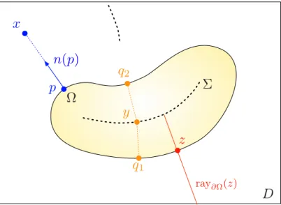
Let us recall a few useful notions and facts related to the signed distance function, see alsoFigure 2:
Σ
<latexit sha1_base64="yjGgDcLCn5bn4lwtIWx04UxiAGk=">AAACyXicjVHLSsNAFD2Nr1pfVZdugkVwVZIqqLuCG8FNRfuAtkgyndaxeZlMxFpc+QNu9cfEP9C/8M4YQS2iE5KcOfeeM3PvdSNPJNKyXnLG1PTM7Fx+vrCwuLS8UlxdayRhGjNeZ6EXxi3XSbgnAl6XQnq8FcXc8V2PN93hoYo3r3mciDA4k6OId31nEIi+YI4kqtE5FQPfOS+WrLKllzkJ7AyUkK1aWHxGBz2EYEjhgyOAJOzBQUJPGzYsRMR1MSYuJiR0nOMOBdKmlMUpwyF2SN8B7doZG9BeeSZazegUj96YlCa2SBNSXkxYnWbqeKqdFfub91h7qruN6O9mXj6xEhfE/qX7zPyvTtUi0ce+rkFQTZFmVHUsc0l1V9TNzS9VSXKIiFO4R/GYMNPKzz6bWpPo2lVvHR1/1ZmKVXuW5aZ4U7ekAds/xzkJGpWyvVOunOyWqgfZqPPYwCa2aZ57qOIINdTJ+xIPeMSTcWxcGTfG7Ueqkcs06/i2jPt3hkKRfw==</latexit>D
<latexit sha1_base64="goRwTPpypAxgaDqCMmIv3G2okJI=">AAACxHicjVHLSsNAFD2Nr1pfVZdugkVwVZIqqLuCIi5bsK1QiyTTaQ3Ni8lEKEV/wK1+m/gH+hfeGaegFtEJSc6ce8+Zuff6aRhk0nFeC9bc/MLiUnG5tLK6tr5R3txqZ0kuGG+xJEzEle9lPAxi3pKBDPlVKrgX+SHv+KNTFe/ccZEFSXwpxynvRd4wDgYB8yRRzbObcsWpOnrZs8A1oAKzGkn5BdfoIwFDjggcMSThEB4yerpw4SAlrocJcYJQoOMc9yiRNqcsThkesSP6DmnXNWxMe+WZaTWjU0J6BSlt7JEmoTxBWJ1m63iunRX7m/dEe6q7jenvG6+IWIlbYv/STTP/q1O1SAxwrGsIqKZUM6o6Zlxy3RV1c/tLVZIcUuIU7lNcEGZaOe2zrTWZrl311tPxN52pWLVnJjfHu7olDdj9Oc5Z0K5V3YNqrXlYqZ+YURexg13s0zyPUMcFGmhp70c84dk6t0Irs/LPVKtgNNv4tqyHD+4mj0Q=</latexit>Ω
<latexit sha1_base64="OhBWeFN0+AzER+eMtTFkKHOH7JA=">AAACyXicjVHLSsNAFD2Nr1pfVZdugkVwVZIqqLuCG8GFFewD2iKTdFpj83IyEWtx5Q+41R8T/0D/wjtjBLWITkhy5tx7zsy914l9L5GW9ZIzpqZnZufy84WFxaXlleLqWiOJUuHyuhv5kWg5LOG+F/K69KTPW7HgLHB83nSGhyrevOYi8aLwTI5i3g3YIPT6nsskUY3OScAH7LxYssqWXuYksDNQQrZqUfEZHfQQwUWKABwhJGEfDAk9bdiwEBPXxZg4QcjTcY47FEibUhanDEbskL4D2rUzNqS98ky02qVTfHoFKU1skSaiPEFYnWbqeKqdFfub91h7qruN6O9kXgGxEhfE/qX7zPyvTtUi0ce+rsGjmmLNqOrczCXVXVE3N79UJckhJk7hHsUFYVcrP/tsak2ia1e9ZTr+qjMVq/ZulpviTd2SBmz/HOckaFTK9k65crpbqh5ko85jA5vYpnnuoYoj1FAn70s84BFPxrFxZdwYtx+pRi7TrOPbMu7fAXM0kXc=</latexit> • <latexit sha1_base64="pXkActCnptZX5e3i8T2Zzct4Moo=">AAACynicjVHLSsNAFD2Nr1pfVZdugkVwFZIq6LLgxoWLCvYBtkgyndbQyYPJRCjFnT/gVj9M/AP9C++MKahFdEKSM+eec2fuvUEqwky57mvJWlhcWl4pr1bW1jc2t6rbO+0sySXjLZaIRHYDP+MijHlLhUrwbiq5HwWCd4LxmY537rjMwiS+UpOU9yN/FIfDkPmKqE4vyIXg6qZacx3XLHseeAWooVjNpPqCHgZIwJAjAkcMRVjAR0bPNTy4SInrY0qcJBSaOMc9KuTNScVJ4RM7pu+IdtcFG9Ne58yMm9Epgl5JThsH5ElIJwnr02wTz01mzf6We2py6rtN6B8UuSJiFW6J/cs3U/7Xp2tRGOLU1BBSTalhdHWsyJKbruib21+qUpQhJU7jAcUlYWacsz7bxpOZ2nVvfRN/M0rN6j0rtDne9S1pwN7Pcc6Ddt3xjpz65XGt4RSjLmMP+zikeZ6ggXM00TJVPuIJz9aFJa2JNf2UWqXCs4tvy3r4ABJUkhU=</latexit>z
<latexit sha1_base64="gU4nxfnueWdCoCbCKL7RHo6KEEY=">AAACxHicjVHLSsNAFD2Nr1pfVZdugkVwFSatre2uIIjLFuwDapEkndbQvEgmQi36A27128Q/0L/wzpiCLopOSHLn3HPOzL3Xjjw3EYy957SV1bX1jfxmYWt7Z3evuH/QTcI0dnjHCb0w7ttWwj034B3hCo/3o5hbvu3xnj29kPnePY8TNwyuxSziQ9+aBO7YdSxBUPvhtlhiRqNerTKmM8M0K6xao4CVG7W6qZsGU6uEbLXC4htuMEIIByl8cAQQFHuwkNAzgAmGiLAh5oTFFLkqz/GIAmlTYnFiWIRO6Tuh3SBDA9pLz0SpHTrFozcmpY4T0oTEiymWp+kqnypniS7znitPebcZ/e3MyydU4I7Qv3QL5n91shaBMeqqBpdqihQiq3Myl1R1Rd5c/1GVIIeIMBmPKB9T7Cjlos+60iSqdtlbS+U/FFOicu9k3BSf8pY04MUU9eVBt2yYFaPcPis1G9mo8zjCMU5pnudo4gotdJT3M17wql1qnpZo6TdVy2WaQ/xa2tMXDb2Pvw==</latexit>•
<latexit sha1_base64="Ybys71TCatAMG0HJ1FLJQlWpDlA=">AAACynicjVHLTsJAFD3UF+ILdemmkZi4aqYoCjsTNy5cYCJCAsa0ZcCGoW2mUxNC3PkDbvXDjH+gf+GdsSS6IDpN2zvnnnNm7r1+IsJUMfZesBYWl5ZXiqultfWNza3y9s5NGmcy4K0gFrHs+F7KRRjxlgqV4J1Ecm/sC972R+c6337gMg3j6FpNEn479oZROAgDTxHU7vmZEFzdlSvMadRrNcZs5rjuEaudUMCqjZO6a7sOM6uCfDXj8ht66CNGgAxjcERQFAt4SOnpwgVDQtgtpoRJikKT53hEibQZsTgxPEJH9B3SrpujEe21Z2rUAZ0i6JWktHFAmph4kmJ9mm3ymXHW6DzvqfHUd5vQ38+9xoQq3BP6l27G/K9O16IwQN3UEFJNiUF0dUHukpmu6JvbP6pS5JAQpuM+5SXFgVHO+mwbTWpq1731TP7DMDWq90HOzfCpb0kDnk3Rnh/cVB33yKleHVfOGvmoi9jDPg5pnqc4wwWaaJkqn/GCV+vSktbEmn5TrUKu2cWvZT19AbTckmU=</latexit> ray∂Ω(z) <latexit sha1_base64="N6YNXHQlMWZ7s30FDFn2DUtYddk=">AAAC43icjVFNT9tAEH24FFJoIbTHSpXVqBK9WOtAILlF6qU3UolApCSK1s6SrvCX1mtEiHLrrbeqV/4A1/JfEP8A/gWziyO1B1TWsj375r23OzNBFslcM3a75LxYfrmyWnm1tv76zcZmdevtUZ4WKhTdMI1S1Qt4LiKZiK6WOhK9TAkeB5E4Dk6/mPzxmVC5TJNDPc3EMOaTRJ7IkGuCRtUPAy3O9Uzx6Xw0G2RcacmjwUEsJny+ffF5VK0xr9VsNBhzmef7O6yxRwGrt/aavut7zK4aytVJqzcYYIwUIQrEEEigKY7AkdPThw+GjLAhZoQpiqTNC8yxRtqCWIIYnNBT+k5o1y/RhPbGM7fqkE6J6FWkdPGJNCnxFMXmNNfmC+ts0Ke8Z9bT3G1K/6D0ignV+E7o/3QL5nN1phaNEzRtDZJqyixiqgtLl8J2xdzc/asqTQ4ZYSYeU15RHFrlos+u1eS2dtNbbvN3lmlQsw9LboF7c0sa8GKK7tPBUd3zd7z6t91ae7ccdQXv8RHbNM99tPEVHXTJ+weu8AfXjnB+Or+c349UZ6nUvMM/y7l8ADQ3nKg=</latexit>•
<latexit sha1_base64="lMdOa9TD5ljLWmTIU72zqtpj1pg=">AAACynicjVHLSsNAFD2Nr1pfVZdugkVwVZJaaLMruHHhooJ9QFskSac1dPJgMhFKcecPuNUPE/9A/8I7Ywq6KDohyZlzz7kz914v4UEqLeu9YKytb2xuFbdLO7t7+wflw6NuGmfCZx0/5rHoe27KeBCxjgwkZ/1EMDf0OOt5s0sV7z0wkQZxdCvnCRuF7jQKJoHvSqJ6Qy/jnMm7csWqWnqZBJy67dQIOE7DbjqmnYcqyFc7Lr9hiDFi+MgQgiGCJMzhIqVnABsWEuJGWBAnCAU6zvCIEnkzUjFSuMTO6Dul3SBnI9qrnKl2+3QKp1eQ08QZeWLSCcLqNFPHM51ZsatyL3ROdbc5/b08V0isxD2xf/mWyv/6VC0SEzR1DQHVlGhGVefnWTLdFXVz80dVkjIkxCk8prgg7Gvnss+m9qS6dtVbV8c/tFKxau/n2gyf6pY04OUUzdWgW6vaF9XaTb3ScvJRF3GCU5zTPBto4QptdHSVz3jBq3FtCGNuLL6lRiH3HOPXMp6+ALD7kmQ=</latexit>x
<latexit sha1_base64="AA0ptFJ+phTxfBEAgfCwuf6EHqM=">AAACxHicjVHLSsNAFD2Nr1pfVZdugkVwVZJaaLMrCOKyBdsKtUiSTuvQvJhMxFL0B9zqt4l/oH/hnTEFXRSdkOTMufecmXuvlwQ8lZb1XjBWVtfWN4qbpa3tnd298v5BL40z4bOuHwexuPbclAU8Yl3JZcCuE8Hc0AtY35ueq3j/nomUx9GVnCVsGLqTiI+570qiOg+35YpVtfQyCTh126kRcJyG3XRMOw9VkK92XH7DDUaI4SNDCIYIknAAFyk9A9iwkBA3xJw4QYjrOMMjSqTNKItRhkvslL4T2g1yNqK98ky12qdTAnoFKU2ckCamPEFYnWbqeKadFbvMe6491d1m9Pdyr5BYiTti/9ItMv+rU7VIjNHUNXCqKdGMqs7PXTLdFXVz80dVkhwS4hQeUVwQ9rVy0WdTa1Jdu+qtq+MfOlOxau/nuRk+1S1pwIspmstBr1a1z6q1Tr3ScvJRF3GEY5zSPBto4RJtdLX3M17walwYgZEa2XeqUcg1h/i1jKcvBRyPvA==</latexit>•
<latexit sha1_base64="lMdOa9TD5ljLWmTIU72zqtpj1pg=">AAACynicjVHLSsNAFD2Nr1pfVZdugkVwVZJaaLMruHHhooJ9QFskSac1dPJgMhFKcecPuNUPE/9A/8I7Ywq6KDohyZlzz7kz914v4UEqLeu9YKytb2xuFbdLO7t7+wflw6NuGmfCZx0/5rHoe27KeBCxjgwkZ/1EMDf0OOt5s0sV7z0wkQZxdCvnCRuF7jQKJoHvSqJ6Qy/jnMm7csWqWnqZBJy67dQIOE7DbjqmnYcqyFc7Lr9hiDFi+MgQgiGCJMzhIqVnABsWEuJGWBAnCAU6zvCIEnkzUjFSuMTO6Dul3SBnI9qrnKl2+3QKp1eQ08QZeWLSCcLqNFPHM51ZsatyL3ROdbc5/b08V0isxD2xf/mWyv/6VC0SEzR1DQHVlGhGVefnWTLdFXVz80dVkjIkxCk8prgg7Gvnss+m9qS6dtVbV8c/tFKxau/n2gyf6pY04OUUzdWgW6vaF9XaTb3ScvJRF3GCU5zTPBto4QptdHSVz3jBq3FtCGNuLL6lRiH3HOPXMp6+ALD7kmQ=</latexit>p
<latexit sha1_base64="fOdhaLZPeXOdXS7LIzL/z4GodAk=">AAACxHicjVHLSsNAFD2Nr1pfVZdugkVwVZJaaLMrCOKyBfuAWiRJpzU0LyYToRT9Abf6beIf6F94Z5yCLopOSHLm3HvOzL3XS8MgE5b1XjDW1jc2t4rbpZ3dvf2D8uFRL0ty7rOun4QJH3huxsIgZl0RiJANUs7cyAtZ35tdynj/gfEsSOIbMU/ZKHKncTAJfFcQ1UnvyhWraqllEnDqtlMj4DgNu+mYtg5VoFc7Kb/hFmMk8JEjAkMMQTiEi4yeIWxYSIkbYUEcJxSoOMMjSqTNKYtRhkvsjL5T2g01G9NeemZK7dMpIb2clCbOSJNQHicsTzNVPFfOkl3lvVCe8m5z+nvaKyJW4J7Yv3TLzP/qZC0CEzRVDQHVlCpGVudrl1x1Rd7c/FGVIIeUOInHFOeEfaVc9tlUmkzVLnvrqviHypSs3Ps6N8envCUNeDlFczXo1ar2RbXWqVdajh51ESc4xTnNs4EWrtFGV3k/4wWvxpURGpmRf6caBa05xq9lPH0B8g2PtA==</latexit>•
<latexit sha1_base64="AL4iABsBFbCZJVa7IaUMdgDlfD8=">AAACynicjVHLSsNAFD3Gd31VXboJFsFVmNhWm13BjQsXCrYVtEiSTjU4eTCZCKW48wfc6oeJf6B/4Z0xBV0UnZDkzrnnnJl7b5CJKFeMvc9Ys3PzC4tLy5WV1bX1jermVjdPCxnyTpiKVF4Gfs5FlPCOipTgl5nkfhwI3gvuj3W+98BlHqXJhRplvB/7t0k0jEJfEdS7DgohuLqp1pjjeazeatjMaR7WG8yjgDVdt+XarsPMqqFcZ2n1DdcYIEWIAjE4EiiKBXzk9FzBBUNGWB9jwiRFkclzPKJC2oJYnBg+off0vaXdVYkmtNeeuVGHdIqgV5LSxh5pUuJJivVptskXxlmj07zHxlPfbUT/oPSKCVW4I/Qv3YT5X52uRWGIlqkhopoyg+jqwtKlMF3RN7d/VKXIISNMxwPKS4pDo5z02Taa3NSue+ub/IdhalTvw5Jb4FPfkgY8maI9PegeOG7dOThv1NpeOeol7GAX+zTPI7RxgjN0TJXPeMGrdWpJa2SNv6nWTKnZxq9lPX0BxY6SbA==</latexit>y
<latexit sha1_base64="Mtlk/T/DNxtBw780OgjpTRrskik=">AAACxHicjVHLSsNAFD2Nr1pfVZdugkVwFSZ9aLMrCOKyBfuAWiRJpzWYF8lEKEV/wK1+m/gH+hfeGVPQRdEJSe6ce86Zufc6se+lgrH3grayura+UdwsbW3v7O6V9w96aZQlLu+6kR8lA8dOue+FvCs84fNBnHA7cHzed+4vZL7/wJPUi8JrMYv5KLCnoTfxXFsQ1JndlivMsCxWa9Z1ZjTOanVmUcAaptk0ddNgalWQr3ZUfsMNxojgIkMAjhCCYh82UnqGMMEQEzbCnLCEIk/lOR5RIm1GLE4Mm9B7+k5pN8zRkPbSM1Vql07x6U1IqeOENBHxEorlabrKZ8pZosu858pT3m1Gfyf3CggVuCP0L92C+V+drEVggqaqwaOaYoXI6tzcJVNdkTfXf1QlyCEmTMZjyicUu0q56LOuNKmqXfbWVvkPxZSo3Ls5N8OnvCUNeDFFfXnQqxpmzah26pWWlY+6iCMc45TmeY4WrtBGV3k/4wWv2qXma6mWfVO1Qq45xK+lPX0BHA+PxQ==</latexit>q
1 <latexit sha1_base64="CEXJbdZXb6jX4xKHzQ8d237mhhw=">AAACxnicjVHLTsJAFD3UF+ILdemmkZi4aqY8FHYkblhilEeChLRlwIbS1naqIcTEH3Crn2b8A/0L74wl0QXRadreOfecM3PvtUPPjQVj7xltZXVtfSO7mdva3tndy+8ftOMgiRzecgIviLq2FXPP9XlLuMLj3TDi1tT2eMeeXMh8555HsRv412IW8v7UGvvuyHUsQdDV3cAc5AvMqNVYqVrWmVE5K5VZjQJWMc2qqZsGU6uAdDWD/BtuMEQABwmm4PAhKPZgIaanBxMMIWF9zAmLKHJVnuMROdImxOLEsAid0HdMu16K+rSXnrFSO3SKR29ESh0npAmIF1EsT9NVPlHOEl3mPVee8m4z+tup15RQgVtC/9ItmP/VyVoERqiqGlyqKVSIrM5JXRLVFXlz/UdVghxCwmQ8pHxEsaOUiz7rShOr2mVvLZX/UEyJyr2TchN8ylvSgBdT1JcH7aJhloziZblQr6WjzuIIxzileZ6jjgaaaJH3GM94wavW0Hwt0R6+qVom1Rzi19KevgCr4ZBh</latexit>q
2 <latexit sha1_base64="EETOElUI8pJrV+RL+sfRhxPdOy0=">AAACxnicjVHLTsJAFD3UF+ILdemmkZi4aqY8FHYkblhilEeChLRlwIbS1naqIcTEH3Crn2b8A/0L74wl0QXRadreOfecM3PvtUPPjQVj7xltZXVtfSO7mdva3tndy+8ftOMgiRzecgIviLq2FXPP9XlLuMLj3TDi1tT2eMeeXMh8555HsRv412IW8v7UGvvuyHUsQdDV3aA4yBeYUauxUrWsM6NyViqzGgWsYppVUzcNplYB6WoG+TfcYIgADhJMweFDUOzBQkxPDyYYQsL6mBMWUeSqPMcjcqRNiMWJYRE6oe+Ydr0U9WkvPWOldugUj96IlDpOSBMQL6JYnqarfKKcJbrMe6485d1m9LdTrymhAreE/qVbMP+rk7UIjFBVNbhUU6gQWZ2TuiSqK/Lm+o+qBDmEhMl4SPmIYkcpF33WlSZWtcveWir/oZgSlXsn5Sb4lLekAS+mqC8P2kXDLBnFy3KhXktHncURjnFK8zxHHQ000SLvMZ7xgletoflaoj18U7VMqjnEr6U9fQGuQZBi</latexit>•
<latexit sha1_base64="AL4iABsBFbCZJVa7IaUMdgDlfD8=">AAACynicjVHLSsNAFD3Gd31VXboJFsFVmNhWm13BjQsXCrYVtEiSTjU4eTCZCKW48wfc6oeJf6B/4Z0xBV0UnZDkzrnnnJl7b5CJKFeMvc9Ys3PzC4tLy5WV1bX1jermVjdPCxnyTpiKVF4Gfs5FlPCOipTgl5nkfhwI3gvuj3W+98BlHqXJhRplvB/7t0k0jEJfEdS7DgohuLqp1pjjeazeatjMaR7WG8yjgDVdt+XarsPMqqFcZ2n1DdcYIEWIAjE4EiiKBXzk9FzBBUNGWB9jwiRFkclzPKJC2oJYnBg+off0vaXdVYkmtNeeuVGHdIqgV5LSxh5pUuJJivVptskXxlmj07zHxlPfbUT/oPSKCVW4I/Qv3YT5X52uRWGIlqkhopoyg+jqwtKlMF3RN7d/VKXIISNMxwPKS4pDo5z02Taa3NSue+ub/IdhalTvw5Jb4FPfkgY8maI9PegeOG7dOThv1NpeOeol7GAX+zTPI7RxgjN0TJXPeMGrdWpJa2SNv6nWTKnZxq9lPX0BxY6SbA==</latexit>•
<latexit sha1_base64="AL4iABsBFbCZJVa7IaUMdgDlfD8=">AAACynicjVHLSsNAFD3Gd31VXboJFsFVmNhWm13BjQsXCrYVtEiSTjU4eTCZCKW48wfc6oeJf6B/4Z0xBV0UnZDkzrnnnJl7b5CJKFeMvc9Ys3PzC4tLy5WV1bX1jermVjdPCxnyTpiKVF4Gfs5FlPCOipTgl5nkfhwI3gvuj3W+98BlHqXJhRplvB/7t0k0jEJfEdS7DgohuLqp1pjjeazeatjMaR7WG8yjgDVdt+XarsPMqqFcZ2n1DdcYIEWIAjE4EiiKBXzk9FzBBUNGWB9jwiRFkclzPKJC2oJYnBg+off0vaXdVYkmtNeeuVGHdIqgV5LSxh5pUuJJivVptskXxlmj07zHxlPfbUT/oPSKCVW4I/Qv3YT5X52uRWGIlqkhopoyg+jqwtKlMF3RN7d/VKXIISNMxwPKS4pDo5z02Taa3NSue+ub/IdhalTvw5Jb4FPfkgY8maI9PegeOG7dOThv1NpeOeol7GAX+zTPI7RxgjN0TJXPeMGrdWpJa2SNv6nWTKnZxq9lPX0BxY6SbA==</latexit>n(p)
<latexit sha1_base64="buK7exuRoc7uCjqY2dP9Pi6tEZc=">AAACx3icjVHLTsJAFD3UF+ILdemmkZjghrRoIuxI3OgOE3kkSExbBpjQV6ZTIiEu/AG3+mfGP9C/8M5YEl0QnabtnXPPOTP3Xjf2eSIt6z1nrKyurW/kNwtb2zu7e8X9g3YSpcJjLS/yI9F1nYT5PGQtyaXPurFgTuD6rONOLlW+M2Ui4VF4K2cx6wfOKORD7jlSQWE5Pr0vlqyKpZf5I6jXa1XLNu0MKSFbzaj4hjsMEMFDigAMISTFPhwk9PRgw0JMWB9zwgRFXOcZHlEgbUosRgyH0Al9R7TrZWhIe+WZaLVHp/j0ClKaOCFNRDxBsTrN1PlUOyt0mfdce6q7zejvZl4BoRJjQv/SLZj/1alaJIao6Ro41RRrRFXnZS6p7oq6ufmjKkkOMWEqHlBeUOxp5aLPptYkunbVW0fnPzRToWrvZdwUn+qWNODFFM3lQbtasc8q1ZvzUqOejTqPIxyjTPO8QANXaKJF3mM84wWvxrURGVPj4Ztq5DLNIX4t4+kL0ceQag==</latexit>Figure 2. Illustration of the main objects attached to the signed distance function. The point x∈ D \ Σ has p ∈ ∂Ω as unique projection point, while y ∈ Σ has q1 and q2 for projections onto
∂Ω.
(i) the set of points p where the infimum is realized in(2.8)is the set of projections of x onto ∂Ω. When there exists a unique such point, it is called the projection of x onto ∂Ω, and it is denoted by p∂Ω(x);
(ii) the set of points x ∈ D having at least two distinct projections onto ∂Ω is called the skeleton (or sometimes, the medial axis) Σ of Ω. It is a set with null Lebesgue measure, and since Ω is smooth, so is the closure Σ, see [33,63];
(iii) the set of points x ∈ D \ Σ sharing the same projection point z ∈ ∂Ω is called the normal ray of z:
ray∂Ω(z) = {x ∈ D \ Σ, p∂Ω(x) = z} ; (2.9)
(iv) the signed distance function is differentiable at every point x ∈ D \ Σ, and its derivative reads: ∇dΩ(x) = n(p∂Ω(x)).
The signed distance function dΩ conveniently encodes most of the geometric features of the domain Ω.
We refer to [33] for an extensive discussion of this notion, and to Section 1.3 in [40] for an introduction. The geometric constraints of interest in this work assume the form:
P (Ω) ≤ 0 where P (Ω) := Z
D
j(dΩ(x))dx, (2.10)
for a given smooth function j : R → R; see sections 3.2.2 and 4.3 for several instances of such geometric constraints.
As we have seen insections 2.2and2.3, the solution of the optimization program(2.1)relies on the shape derivative DP (Ω) of P . The numerical computation of the shape derivative of functions P (Ω) of the form
(2.10), depending on the signed distance function dΩ, requires a special treatment which we now summarize,
referring to [4,68,10] for details. The shape derivative of P (Ω) reads: DP (Ω)(θ) =
Z
D
j′(dΩ(x))d′Ω(θ)(x)dx. (2.11)
In the above expression, d′
Ω(θ) is the “Eulerian derivative” of the signed distance function in the direction
θ∈ W1,∞(D, Rd), that is, for a.e. x ∈ D, d′
Ω(θ)(x) is the Fr´echet derivative of the mapping θ 7→ dΩ(θ)(x)
at θ = 0. This function satisfies the following boundary-value problem: (∇d′
Ω(θ) · ∇dΩ= 0 in D\Σ
d′Ω(θ) = −θ · n on ∂Ω,
(2.12)
where n denotes the normal vector to ∂Ω, pointing outward Ω. The first line of (2.12) expresses that the values of d′
Ω(θ) are constant along the rays(2.9)of ∂Ω, while the second line actually specifies these values
on ∂Ω.
The expression(2.11)is uneasy to handle in practice, since the derivative d′Ω(θ) depends in a non-trivial
way on θ. Owing to the coarea formula,(2.11)can be rewritten in the following surface form: DP (Ω)(θ) =
Z
∂Ω
vP(Ω)θ · n ds; (2.13)
see [4, 10, 44]. Unfortunately, the analytical expression of the scalar field vP(Ω) : Γ → R (which is not
reported here for brevity) involves integrals along the normal rays to ∂Ω, as well as the principal curvatures of ∂Ω. These quantities are well-known to be difficult to compute in a robust way on unstructured meshes. These issues can be overcome thanks to the variational method from our previous work [44]: instead of evaluating the analytic formula for the function vP(Ω), we actually compute it numerically as the solution
to a variational problem. More precisely, we consider the problem find v ∈ Vωsuch that for any w ∈ Vω,
Z ∂Ω vw ds + Z D\Σ ω(∇dΩ· ∇v)(∇dΩ· ∇w) dx = − Z D j′(dΩ)w dx, (2.14)
which is easily solved numerically by means of standard piecewise linear finite elements. In the above formulation, the function ω is a positive weight which is continuous on D\Σ, while Vωis a weighted Hilbert
space, whose precise definition and mathematical properties are described in Section 2 of [44].
The space Vω contains functions w which are constant along the sets ray∂Ω(z), z ∈ ∂Ω, and possibly
discontinuous across Σ. Recalling(2.12), one may then insert d′
Ω(θ) as test function in(2.14), and it follows
from the expression(2.12)that the trace of the solution v ∈ Vω to (2.14)on Γ is exactly the desired scalar
field vP(Ωf).
The weight ω can be chosen rather arbitrarily. In theory, from [44], it should only be continuous and positive on D\Σ and satisfy a few additional monotonicity assumptions. It is however numerically desirable that ω vanish on the skeleton Σ of Ω so that the discontinuities of test functions w ∈ Vωacross Σ are better
captured with piecewise linear finite elements, thus enhancing the accuracy of the calculation of vP(Ωf). In
all the situations addressed in this work, following the recommendation in [44] (section 3.3.1) we use the weight
ω = 2
1 + 100|dΩ∆dΩ|3.5
,
a choice which is motivated by the large values of the discretized version of ∆dΩ near Σ. The constants 100
or 3.5 have been selected empirically to achieve universally satisfactory performance even when the distance of ∂Ω to the skeleton Σ is small. In most cases, the use of different constants works equally well.
2.5. Topology optimization using a level-set based mesh evolution method
Among the multiple available approaches, see [7] for an overview, we rely on the level-set based mesh evolution algorithm from our previous works [5, 6, 42, 45] for the numerical representation of shapes and their deformations, see also [77] for earlier related ideas. The salient feature of this approach is that it enjoys an explicit, meshed representation of the tracked subdomains Ωf and Ωs at any stage of the optimization
process, while still allowing for topological changes. This is possible thanks to the combination of two complementary numerical representations of the partition D = Ωf∪ Ωs:
(i) a meshed description: a conforming simplicial mesh T , i.e., composed of triangles in 2D and tetrahedra in 3D, of the total domain D is available, in which the interface Γ is meshed explicitly. This repre-sentation is well-suited when it comes to solving the physical state equations with the finite element method on their associated meshed subdomains Ωf and Ωs, see, e.g.,Figs. 5,12and23din the results
below;
(ii) a level-set description: following the pioneering work [73], see also [82] for an overview and [12,89,83,74] for the seminal applications in shape and topology optimization, Ωf and Ωsare represented by means
of a scalar function φ : D → R, in practice discretized at the vertices of a mesh of D, such that: φ(x) < 0 if x ∈ Ωf φ(x) = 0 if x ∈ Γ φ(x) > 0 if x ∈ Ωs.
This representation allows to account for large deformations of the configuration D = Ωf∪Ωsaccording
to a given velocity field θ and a pseudo-time step τ > 0. One solves to this end the following linearized version of the level-set advection equation:
∂ψ ∂t(t, x) + θ(x) · ∇ψ(t, x) = 0 (t, x) ∈ (0, τ ) × D ψ(0, x) = φ(x) x ∈ D, (2.15)
which yields an updated level-set function ψ(τ, ·) associated to the partition D = (Ωf)τ θ∪ (Ωs)τ θ,
where (Ωf)τ θ is the negative subdomain of φ(τ, ·) and (Ωs)τ θ := D\(Ωf)τ θ.
Dedicated numerical algorithms allow to switch from one of these descriptions to the other. On the one hand, a level-set function φ associated to a configuration D = Ωf ∪ Ωs under meshed description is
generated as the signed distance function to Ωf by using the open-source software Mshdist [28]. Conversely,
a conforming mesh of D where both subdomains Ωf and Ωs are explicitly discretized is generated from the
datum of an associated level-set function φ : D → R thanks to the remeshing library Mmg [27, 26], see also the aforementioned works [5, 6,42,45] for illustrations and details.
2.6. The complete algorithmic procedure
The shape and topology optimization algorithm derived from the previous considerations is summarized in
algorithm 1 below. Note that we refer to our method as a “shape and topology optimization algorithm”
(although we rely solely on shape derivatives) because the boundaries of the design domain are allowed to move freely and topological changes occurring in the course of the optimization are captured. Our approach is therefore substantially different from the many works concerned with parametric shape optimization of fluid systems [49,39,23,38], whereby very small updates of the design shape are sought.
Algorithm 1 Body-fitted topology optimization algorithm ofsection 2. input: conforming initial mesh T0of D, where Ω0
f and Ω0sappear explicitly as meshed subdomains
for n = 0, 1, 2, . . . until convergence do
(1) generate the signed distance function φn to Ωn
f on the whole mesh Tn;
(2) compute the physical states v(Ωn
f), p(Ωnf), and T (Ωnf) as well as the corresponding adjoint
states by solving the coupled Navier–Stokes and convection–diffusion equations on Tn, taking
advantage of the associated submeshes for Ωn
f and Ωns;
(3) compute a deformation field θnwhich decreases the value of J and the violation of the constraints
gi and hj thanks to the optimization algorithm insection 2.3.
(4) solve the level-set advection equation (2.15) on Tn, for a suitably small time period [0, τn]: a
level-set function for the new partition D = Ωn+1f ∪ Ωn+1s is obtained as φn+1:= ψ(τn, ·);
(5) construct a new conforming mesh Tn+1 of D in which both subdomains Ωn+1
f and Ωn+1s are
explicitly discretized. end for
return optimized partition D = Ωn f ∪ Ωns.
3. Topology optimization of a 2D air–oil heat exchanger
In this section, we deal with the optimization of the 2D cross-section of a three-dimensional air–oil heat exchanger. The setting of this problem is described in section 3.1. The two phases Ωf and Ωs are filled
with air and oil, respectively. The physical phenomena of interest solely take place in Ωf: the velocity and
pressure (v, p) of the fluid are governed by the 2D incompressible steady-state Navier–Stokes equations, and the temperature T inside Ωf is subject to diffusion and convection by the fluid, with a thermostatic boundary
condition on the interface Γ. The optimization problem is formulated in section 3.2, where we define the considered shape functionals, and notably a minimum thickness constraint imposed on the oil phase Ωs.
Section 3.3 presents a variety of numerical results, obtained by applying algorithm 1 with different initial
designs and sets of physical parameters.
Remark 1. Here and in the sequel, physical units are omitted when it comes to the numerical values used in our test cases. For simplicity, we prefer to work with nondimensional quantities, and we do not claim that all values are completely relevant from the physical point of view. In particular, because of computational limitations, our choices of Reynolds and P´eclet numbers (which are nondimensional in the first place) are quite restricted to moderate values. Nevertheless, one can think that the physical units are SI units as follows. All lengths are understood in meters (m), velocities in m s−1, temperatures in Kelvin (K) or degree Celsius
in the next sections, fluid density in kg m−3, fluid thermal capacity in J K−1kg−1, thermal conductivity in
J K−1m−1s−1, and fluid viscosity in kg m−1s−1.
3.1. Setting of the study
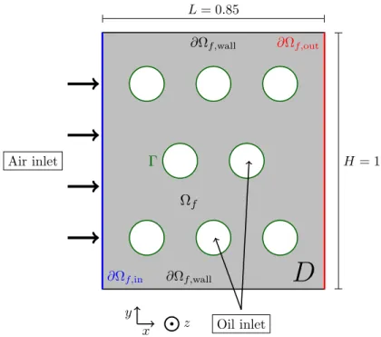
Our purpose is to optimize the shape and the topology of a 2D air–oil heat exchanger. The situation is that depicted onFigure 3: the hold-all domain D = (0, L) × (0, H) is a rectangle with width L = 0.85 and height H = 1. It contains a fluid, air, which occupies a subdomain Ωf ⊂ D to be optimized. The complementary
subdomain Ωs= D \ Ωf is filled with oil. The fluid boundary
∂Ωf = ∂Ωf,in∪ ∂Ωf,out∪ ∂Ωf,wall∪ Γ,
is composed of the following regions:
• ∂Ωf,in is the inlet boundary, where the fluid is entering the device with a parabolic velocity v0 with
maximum norm ||v0||∞;
• ∂Ωf,out is the outlet boundary, where the fluid is exiting the device with zero normal stress;
• ∂Ωf,wallis the remaining part of the device D, which bears a no-slip boundary condition for the fluid
and an adiabatic boundary condition for the temperature;
• Γ = Ωf ∩ Ωs is the interface between the air and oil phases. The oil inside Ωs has a much higher
thermal conductivity than that of air, and so the temperature takes the uniform value T = Toilin Ωs.
Moreover, the interface Γ is sufficiently thin and conductive so that T = Toilon Γ.
From a physical point of view, after 3D extrusion in the z-direction, this system can be interpreted as a heat exchanger featuring air flowing in the x-direction and cooling down infinitely long oil channels flowing in the transverse z-direction.
H = 1 L = 0.85
D
Ω
f Air inlet Oil inlet ∂Ωf,in ∂Ωf,outΓ
∂Ωf,wall ∂Ωf,wall x y zFigure 3. Setting of the air–oil heat exchanger ofsection 3.
Mathematically, the fluid, air, is characterized by its velocity v and pressure p in Ωf, which are the
solutions to the incompressible steady-state Navier–Stokes equations: −div(σf(v, p)) + ρ∇v v = 0 in Ωf div(v) = 0 in Ωf v = v0 on ∂Ωf,in σf(v, p)n = 0 on ∂Ωf,out v = 0 on ∂Ωf,wall v = 0 on Γ. (3.1)
Here, ρ is the fluid density, and the fluid stress tensor σf(v, p) is given by Newton’s law:
σf(v, p) = 2νe(v) − pI, (3.2)
in which e(v) = 1
2(∇v + ∇vT) is the rate of strain tensor, ν is the dynamic viscosity of the fluid, and I is
the identity 2 × 2 matrix. The temperature field T inside the air phase Ωf is then determined in terms of
the velocity v through the following convection–diffusion equation: −div(kf∇T ) + ρcpv· ∇T = 0 in Ωf T = Tin on ∂Ωf,in −kf ∂T ∂n = 0 on ∂Ωf\∂Ωf,in T = Toil on Γ, (3.3)
where kf and cp are the thermal conductivity and the thermal capacity of the fluid, respectively. Let us
emphasize that, thanks to the thermostatic boundary condition T = Toilimposed on the interface Γ, no model
is needed for describing the motion of the oil phase in Ωs, and the coupled system of physical equations(3.1)
and(3.3)is posed solely on Ωf.
In our application, the “cold” air flow is entering the domain D on the left-hand side with a temperature Tin= 310. The temperature on the interface Γ is set to Toil= 400. The density and the capacity coefficients
of the fluid are ρ = 1 and cp = 1. Since we do not rely on a turbulence model in the Navier–Stokes equations 11
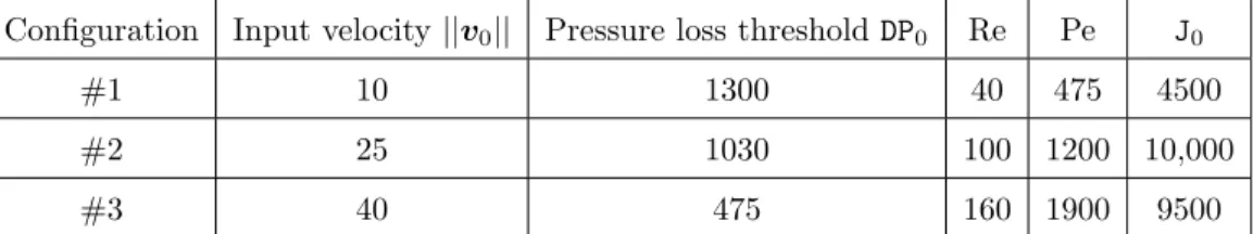
Configuration Input velocity ||v0|| Pressure loss threshold DP0 Re Pe J0
#1 10 1300 40 475 4500
#2 25 1030 100 1200 10,000
#3 40 475 160 1900 9500
Table 1. Configurations considered for the input velocity and pressure constraint values.
(3.1)for the determination of the fluid velocity and pressure (v, p), our study is restricted to moderate values
of Reynolds and P´eclet numbers Re and Pe. The viscosity and conductivity coefficients ν and kf are set so
that the values
Re :=ρ||v0||∞H
ν Pe :=
ρcp||v0||∞H
kf
, are those associated to the three different configurations described inTable 1. 3.2. Formulation of the shape optimization problem
3.2.1. Definition of the objective and constraint functions
In this first physical setting, the heat exchanged between the air, Ωf, and the oil, Ωs, phases is maximized,
while imposing an upper bound DP0 on the static pressure drop between the inlet and the outlet of the
device. The considered shape and topology optimization problem(2.1)reads in this case: min Ωf⊂D J(Ωf) := − Z Ωf ρcpv· ∇T dx s.t. DP(Ωf) := Z ∂Ωf,in pds − Z ∂Ωf,out pds ≤ DP0. (3.4)
Upon integration by parts, the objective function J(Ωf) rewrites exactly as the difference between the heat
entering from the inlet ∂Ωf,in and that exiting from ∂Ωf,out:
J(Ωf) = − Z ∂Ωf,in ρcpT v · nds + Z ∂Ωf,out ρcpT v · nds ! ,
where we recall that the normal vector n is pointing outward D. The first term in the above right-hand side is constant since v = v0 on ∂Ωf,in, so that minimizing J(Ωf) is equivalent to maximizing the heat leaving
the device through ∂Ωf,out, which is also the heat extracted from the oil channels Ωs.
Remark 2. Strictly speaking, sufficient regularity is expected for the pressure p, which is only a priori an element of L2(Ω
f), to have a trace on the inlet and outlet boundaries. The shape derivative of DP(Ωf)
is computed with the formulas of [40], which requires the solution to a fluid adjoint system involving the linearized transpose of the Navier–Stokes operator and a boundary integral involving a pressure test variable as a right-hand side.
3.2.2. Minimum thickness constraint for the oil phase cross-section Ωs
As evidenced by the results of section 3.3 below, the solution of the optimization problem (3.4) tends to produce very thin and elongated patterns for the oil cross-section Ωs. From a physical point of view, these
would induce an important pressure drop in the transverse oil channels of the underlying three-dimensional device, making the overall design impractical. Furthermore, such thin and elongated components are nu-merically instable. Indeed, patterns of the design smaller than the prescribed mesh size tend to disappear in the course of the remeshing steps due to smoothing. This calls for the addition of a constraint on the minimum thickness dminof the oil channels Ωsin the shape optimization problem(3.4), which also improves
the manufacturability of the optimized device. Our modeling of this constraint follows the strategy proposed in [68]: we replace the shape and topology optimization problem(3.4)with a variant where the performance of the system J(Ωf) is constrained to be at least as good as a threshold value J0. The minimized function
E(Ωf) favors areas of D\Ωf thicker than dmin, and its shape derivative vanishes in those regions which are
already thicker than dmin:
min Ωf⊂D E(Ωf) := − Z D\Ωf d2Ωfmax(−dΩf + dmin/2, 0) 2dx s.t. ( DP(Ωf) ≤ DP0 J(Ωf) ≥ J0. (3.5)
In the present setting, the minimum thickness value is set to dmin:= 0.027. As already mentioned, the shape
derivatives of the “mechanical” functionals J(Ωf) and DP(Ωf), depending on Ωf via the solutions v(Ωf),
p(Ωf), and T (Ωf) to the physical equations(3.1)and(3.3), have been calculated in our previous work [42],
and their expressions are omitted for brevity. The shape derivative of the functional E(Ωf), of the form
(2.10), is evaluated numerically with the variational method ofsection 2.4. The threshold J0 measuring the
performance of the heat exchanger is determined empirically from the values obtained from the solution of the original problem (3.4)without the minimum thickness constraint. This value is set depending on the configuration considered according toTable 1.
3.3. Numerical results
We optimize the design of the considered heat exchangers without and with the minimum thickness constraint
ofsection 3.2.2. Namely, we solve both optimization problems(3.4)and(3.5), for the three sets of parameters
of Table 1. In order to further illustrate the strong dependence of optimized designs on the corresponding
initializations, we propose a set of 24 exploratory results, corresponding to 4 different initial topologies and 3 sets of imposed velocities and allowed pressure drops (plus the 2 cases with or without thickness constraint). These are reported inTable 2below where the final temperature and kinetic energy fields are also displayed. Let us note that the existence of different (local) minima which can be obtained by using as many different initializations is often seen as a drawback in mathematical optimization; the present numerical experiment shows, however, that it is rather an advantage from an engineering perspective since it leaves the room for many possible designs which can accommodate other practical constraints, not yet taken into account.
As is visible on Table 2, the maximum pressure drop constraint is not saturated in all the situations where ||v0||∞= 10. In test cases #3, #5, thin structures have been removed due to remeshing in the course
of the optimization process. For some of the other test cases, the topology changes due to the elongation of the oil phase which creates additional connected components (e.g. in #19 and #20 where the number of oil components increases from 5 to 7). Last, in the configurations featuring the minimum thickness constraint formulated as (3.5), the prescribed threshold values J0 and DP0 are often too ambitious. As a
result these constraints are slightly violated by the final design because the optimization algorithm had to find a compromise between the two. This is visible for instance on #24, where the pressure drop DPfinal
is much worse as in the corresponding case #23 where the thickness constraint is not imposed, but which features also a much better heat exchanged Jfinal.
Since the heating of the air flow is due to a Dirichlet boundary condition on the oil channels, the optimiza-tion algorithm has a tendency to increase the length of the oil/air interface, which simultaneously increases the amount of heat exchanged between oil and air. For large velocities, the oil channels are elongated with an aerodynamic profile in order to meet the pressure drop limit. Note that the volume of the oil channels is not constrained and thus varies a lot from one case to another. In some cases, such as #8, #10, #14, #19, #20, #22 and #24, the initial topology is a collection of oil “islands” and it is transformed, after optimization, into a kind of oil “matrix” perforated by air channels. This is a feature of topology optimization algorithms which cannot be achieved in practice by parametric optimization algorithms, even if the geometry of the shape can be modified by moving the mesh. The key point is here the use of a remeshing algorithm which allows for very large mesh deformations.
Remarkably, the optimization algorithm generates recirculating fluid patterns opposed to the direct flow, e.g., on cases #8–#12 and #20–#24, which increase the amount of exchanged heat by widening the surface contact area between the hot oil phase and the incoming flow. Note that [78] has also reported the benefit of recirculating patterns, such as counter-rotating vortices, when it comes to heat exchange. Furthermore, the conducted numerical procedure has selected aerodynamic designs for the transverse oil channels so as to
limit the output pressure loss. Finally, the effect of the minimum thickness constraint in(3.5)is particularly significant on the configurations where the input velocity is maximum, ||v0||∞ = 40, which are also those
favoring the most elongated structures.
A few intermediate shapes illustrating the shape optimization process in some of these experiments are reported inFigs. 4ato4c. Finally, all these results were produced with a rather fine mesh resolution for the bounding box D: the minimum edge size was of the order of hmin = 0.003, which corresponds to meshes
with approximately 30,000 vertices. The whole optimization process of a single test case involves about 400 iterations which took about 12 hours without the use of parallel computing. As an illustration the mesh of the final shape is displayed onFigure 5for one of the 24 situations considered.
Test case T (initial design) T (optimized design) ||v||2 (optimized design) #1 ||v0||∞= 10 DP0= 1300 Jfinal= 4350 DPfinal= 1113 Without min. thickness constraint #2 ||v0||∞= 10 DP0= 1300 Jfinal= 4346 DPfinal= 1217 With min. thickness constraint #3 ||v0||∞= 25 DP0= 1030 Jfinal= 8089 DPfinal= 983 Without min. thickness constraint #4 ||v0||∞= 25 DP0= 1030 Jfinal= 9742 DPfinal= 1030 With min. thickness constraint #5 ||v0||∞= 40 DP0= 475 Jfinal= 3472 DPfinal= 392 Without min. thickness constraint 15
Test case T (initial design) T (optimized design) ||v||2 (optimized design) #6 ||v0||∞= 40 DP0= 475 Jfinal= 7285 DPfinal= 520 With min. thickness constraint #7 ||v0||∞= 10 DP0= 1300 Jfinal= 4086 DPfinal= 1308 Without min. thickness constraint #8 ||v0||∞= 10 DP0= 1300 Jfinal= 4168 DPfinal= 1188 With min. thickness constraint #9 ||v0||∞= 25 DP0= 1030 Jfinal= 7667 DPfinal= 968 Without min. thickness constraint #10 ||v0||∞= 25 DP0= 1030 Jfinal= 7508 DPfinal= 1112 With min. thickness constraint 16
Test case T (initial design) T (optimized design) ||v||2 (optimized design) #11 ||v0||∞= 40 DP0= 475 Jfinal= 5731 DPfinal= 479 Without min. thickness constraint #12 ||v0||∞= 40 DP0= 475 Jfinal= 6847 DPfinal= 524 With min. thickness constraint #13 ||v0||∞= 10 DP0= 1300 Jfinal= 4208 DPfinal= 1140 Without min. thickness constraint #14 ||v0||∞= 10 DP0= 1300 Jfinal= 4252 DPfinal= 1157 With min. thickness constraint #15 ||v0||∞= 25 DP0= 1030 Jfinal= 7785 DPfinal= 1022 Without min. thickness constraint 17
Test case T (initial design) T (optimized design) ||v||2 (optimized design) #16 ||v0||∞= 25 DP0= 1030 Jfinal= 8711 DPfinal= 1106 With min. thickness constraint #17 ||v0||∞= 40 DP0= 475 Jfinal= 6236 DPfinal= 470 Without min. thickness constraint #18 ||v0||∞= 40 DP0= 475 Jfinal= 7822 DPfinal= 498 With min. thickness constraint #19 ||v0||∞= 10 DP0= 1300 Jfinal= 3361 DPfinal= 1149 Without min. thickness constraint #20 ||v0||∞= 10 DP0= 1300 Jfinal= 3582 DPfinal= 1064 With min. thickness constraint 18
Test case T (initial design) T (optimized design) ||v||2 (optimized design) #21 ||v0||∞= 25 DP0= 1030 Jfinal= 2972 DPfinal= 986 Without min. thickness constraint #22 ||v0||∞= 25 DP0= 1030 Jfinal= 5330 DPfinal= 1589 With min. thickness constraint #23 ||v0||∞= 40 DP0= 475 Jfinal= 2847 DPfinal= 476 Without min. thickness constraint #24 ||v0||∞= 40 DP0= 475 Jfinal= 4925 DPfinal= 1051 With min. thickness constraint
Table 2. Topology optimization results for the air–oil heat exchanger case study of section 3
associated to various sets of parameters and initial designs.
4. Design optimization of 2D two-tubes heat exchangers involving a non-mixing constraint This section and the next section 5are devoted to the optimization of a different type of heat exchangers. These are composed of two tubes, containing two different fluids that are separated by a solid phase and must not interpenetrate. The present section is devoted to the 2D case, and the considered physical setting is described insection 4.1. The mathematical formulation of the optimization problem is outlined insection 4.2.
(a) Test case 8, ||v0||∞= 25.
(b) Test case 10, ||v0||∞= 10.
(c) Test case 12, ||v0||∞= 40.
Figure 4. Iterations 0, 10, 20, 100, 200, and 400 of the optimal design process of the 2D air–oil heat exchanger ofsection 3, for several test cases.
Figure 5. Mesh of the final shape in test case 10 of the air–oil heat exchanger optimization example ofsection 3. The diameter of the black circle on the right-hand side corresponds to the prescribed minimum thickness dmin= 0.027.
∂ΩNf
∂ΩN f
d(Ωf,hot,Ωf,cold) ≥ dmin:= 0.15
Ωf,cold Ωf,hot D Ωs Γ ∂ΩD f, Thot ∂ΩD f, Tcold 4 1 2 2 1 10 ∂T ∂n= 0
(a) Counter-current exchange test case: A hot fluid phase Ωf,hot ⊂ D is entering from the upper left side of D with
a temperature Thot, and a cold fluid phase Ωf,coldis entering
in the reverse direction from the lower right inlet.
d(Ωf,hot,Ωf,cold) ≥ dmin:= 0.05 Ωf,cold Γ Ωf,hot D Ωs Tcold Tho t 10 0.5 0.5 1 1 7 10
(b) Co-current exchange test case: a hot fluid phase Ωf,hot⊂ D
is entering from the upper left side of D with a temperature Thot,
and a cold fluid phase Ωf,coldis entering in the same direction
at the lower left inlet (boundary conditions not represented).
Figure 6. Settings of the two test cases considered in the design optimization of the heat exchangers ofsection 4featuring the non-mixing condition d(Ωf,hot,Ωf,cold) ≥ dmin.
The non-penetration constraint between the fluid channels is modeled in section 4.3. Finally, numerical results are presented insection 4.4. 3D results are treated in the next dedicatedsection 5.
4.1. Description of the physical setting
In the present context, the hold-all domain is the square D = (0, 10)2= Ω
s∪ Ωf, which is composed of the
two disjoint fluid and solid phases Ωf and Ωs, respectively. These are separated by the interface Γ = Ωs∩Ωf,
where the fluid satisfies the no-slip boundary condition v = 0. The fluid phase Ωf = Ωf,hot∪ Ωf,cold itself
consists of two distinct channels Ωf,hotand Ωf,coldwhose shapes are to be optimized and kept separated. The
boundary ∂D of the total device D contains the reunion ∂ΩD
f of the inlets of both channels, and the reunion
∂ΩN
f of the outlets. The hot (resp. cold) fluid is entering D through ∂ΩDf ∩ ∂Ωf,hot (resp. ∂ΩDf ∩ ∂Ωf,cold)
with the temperature Thot = 100 (resp. Tcold = 0) and a parabolic velocity profile v0. Both fluids exit D
with vanishing normal stress. The remaining part ∂ΩN := ∂D \ ∂ΩD
f of the boundary of D is adiabatic,
bearing homogeneous Neumann condition ∂T
∂n = 0 for the temperature field T . Both fluids share the same
physical properties: their thermal conductivity kf, thermal capacity cp, kinematic viscosity ν, and density ρ
are equal.
We consider two configurations regarding the location of the inlets, seeFigure 6for an illustration: (i) counter-current exchange test case (Figure 6a): the two liquid phases enter D from opposite sides.
The inlet and outlet cross-sections share a common size a = 2. The initial design is depicted onFigure 7
(left);
(ii) co-current exchange test case (Figure 6b): the two liquid phases enter from the same side of D and the inlet and outlet cross-sections have a smaller common size a = 1. The initial design is that on
Figure 7(right).
The physics involved in this problem are those considered in [42]: the velocity and the pressure (v, p) of the fluid obey the incompressible steady-state Navier–Stokes equations in the total fluid domain Ωf =
Ωf,cold∪ Ωf,hot:
(a) Counter-current exchange test case. (b) Co-current exchange test case.
Figure 7. Initial distribution of the fluid domain Ω0
f (in white) in both test cases considered insection 4.
−div(σf(v, p)) + ρ∇v v = 0 in Ωf div(v) = 0 in Ωf v= v0 on ∂ΩDf σf(v, p)n = 0 on ∂ΩNf v= 0 on Γ, (4.1)
where the viscous stress tensor σf(v, p) is defined by(3.2). The temperature field T is determined by the
equations of convection–diffusion in the reunion of the solid and liquid phases Ωs and Ωf:
−div(kf∇Tf) + ρcpv· ∇Tf = 0 in Ωf −div(ks∇Ts) = 0 in Ωs T = 100 on ∂ΩD f ∩ ∂Ωf,hot T = 0 on ∂ΩDf ∩ ∂Ωf,cold −kf ∂Tf ∂n = 0 on ∂Ω N ∩ ∂Ω f −ks ∂Ts ∂n = 0 on ∂Ω N ∩ ∂Ω s Tf = Ts on Γ −kf ∂Tf ∂n = −ks ∂Ts ∂n on Γ, (4.2)
where Tsand Tf denote the restrictions of T to respectively the solid and the fluid subdomains Ωsand Ωf.
As far as numerical values are concerned, in both test cases, the common density of the fluids is ρ = 1, and their thermal conductivity is kf = 10. The maximum norm of the inlet velocity reads ||v0||∞= 1. The
viscosity ν is computed by the formula ν := ρa||v0||∞/Re where the Reynolds number is set to Re = 60.
Likewise, the capacity coefficient of the fluids is calculated by cp := kfPe/(νRe), where the value of the
P´eclet number is prescribed to Pe = 500. The thermal conductivity of the solid Ωsis chosen to be about ten
times larger than that of the fluids: ks= 110.
4.2. Definition of the objective functional and of the pressure drop constraint
The aim of the optimal design problem is to find the shapes of the “hot” and “cold” components Ωf,hot and
Ωf,coldof the fluid phase Ωf that maximize the heat exchanged between both components. Two constraints
are added on the design: one is about the maximum allowed pressure drop between the inlets and the outlets of the two channels, while the other imposes that Ωf,coldand Ωf,hot do not interpenetrate. The latter
geometric constraint is discussed more thoroughly in the nextsection 4.3.