Publisher’s version / Version de l'éditeur:
Vous avez des questions? Nous pouvons vous aider. Pour communiquer directement avec un auteur, consultez la première page de la revue dans laquelle son article a été publié afin de trouver ses coordonnées. Si vous n’arrivez pas à les repérer, communiquez avec nous à [email protected].
Questions? Contact the NRC Publications Archive team at
[email protected]. If you wish to email the authors directly, please see the first page of the publication for their contact information.
https://publications-cnrc.canada.ca/fra/droits
L’accès à ce site Web et l’utilisation de son contenu sont assujettis aux conditions présentées dans le site LISEZ CES CONDITIONS ATTENTIVEMENT AVANT D’UTILISER CE SITE WEB.
Proceedings of the 2007 IEEE International Joint Conference on Neural Networks
(IJCNN 2007), 2007
READ THESE TERMS AND CONDITIONS CAREFULLY BEFORE USING THIS WEBSITE.
https://nrc-publications.canada.ca/eng/copyright
NRC Publications Archive Record / Notice des Archives des publications du CNRC :
https://nrc-publications.canada.ca/eng/view/object/?id=d13fea8c-4241-487f-9c39-ea80f4dee29b
https://publications-cnrc.canada.ca/fra/voir/objet/?id=d13fea8c-4241-487f-9c39-ea80f4dee29b
NRC Publications Archive
Archives des publications du CNRC
This publication could be one of several versions: author’s original, accepted manuscript or the publisher’s version. / La version de cette publication peut être l’une des suivantes : la version prépublication de l’auteur, la version acceptée du manuscrit ou la version de l’éditeur.
Access and use of this website and the material on it are subject to the Terms and Conditions set forth at
Greenland temperatures and solar activity: a computational intelligence
approach
Greenland Temperatures and Solar Activity:
A Computational Intelligence Approach*
Valdés, J., and Pou, A.
August 12-17, 2007
* Proceedings: 2007 IEEE International Joint Conference on Neural Networks. Orlando, Florida, USA. August 12-17, 2007. NRC 49298.
Copyright 2007 by
National Research Council of Canada
Permission is granted to quote short excerpts and to reproduce figures and tables from this report, provided that the source of such material is fully acknowledged.
Greenland Temperatures and Solar Activity: A Computational
Intelligence Approach
Julio J. Vald´es and Antonio Pou
Abstract— The complexity of the earth’s climate and its rela-tionship with solar activity are here approached by means of two computational intelligence techniques: Multivariate Time Series Model Mining (MVTSMM) and Genetic Programming (GP). They were applied to a temperature record (Delta O18/16), obtained from an ice core in Central Greenland, representative of the climate variations in the North Atlantic regions, and the International Sunspot Number series, as a proxy of solar activity, both covering the period from 1721 to 1983. Several experiments were conducted using these records jointly and separately with the purpose of characterize and reveal their time dependencies.
Preliminary results show this mining approach is a valid and promising research line. The time-lag spectra obtained with MVTSMM seem to point out to time stamps of some of the most important Earth-climate and solar variations, as well as the contribution of solar activity and sunspot solar cycles along time. The GP provided equations which approximate the relative contribution of particular solar time-lags. Although suggestive, this research is at an early stage and the results are preliminary, emphasizing methodological aspects.
I. INTRODUCTION
A large number of studies have focused on the relationship between the solar activity and climate. The presence of a correlation with climate has been widely acknowledged but, due to the large number of intervening processes acting at different spatial and temporal scales, it is extremely difficult to determine a cause-effect relationship. In the present debate on global warming and future climate scenarios, it is of the utmost interest to determine the relative contributions of external forcing mechanisms and anthropogenic changes.
There are inherent difficulties in dealing with external climate forcing mechanisms. The possible physical processes relating them to climate are still obscure and their contribu-tion is part of an ongoing debate. They are extremely difficult to predict and are outside of our control capabilities. So, it is not surprising that most simulation models stay away from them and instead they put the accent on well known climate-related processes [4]. However, solar physicists have been pointing to the extraordinary activity of magnetic solar ejections for the last half century. Some say the activity is without precedent in the last ten thousand years [19] [14], but others disagree [10]. The general consensus is that the Sun is responsible for some general climatic trends, but the
Julio J. Vald´es is with the National Research Council Canada, Insti-tute for Information Technology, 1200 Montreal Rd. Bldg M50, Ottawa, ON K1A 0R6, Canada (phone: 613-993-0887; fax: 613-993-0215; email: [email protected]).
Antonio Pou is with the Department of Ecology, Faculty of Sciences, Au-tonomous University of Madrid, 28049-Madrid, Spain (phone: (34)(91)497-8194; fax: (34)(91)497-8001; email: [email protected]).
abnormal climatic situations we are experiencing, for the last thirty years or so, are believed to be a consequence of anthropogenic activities. Apparently, the solar activity has reached a peak and perhaps has already passed its maximum. This paper explores the use of computational intelligence techniques for time series analysis and model discovery of analytic functions. The purpose is to mine relationships between temperatures on earth and solar activity via two of their proxies: isotope ice core data from Greenland and sunspot numbers.
II. DATA
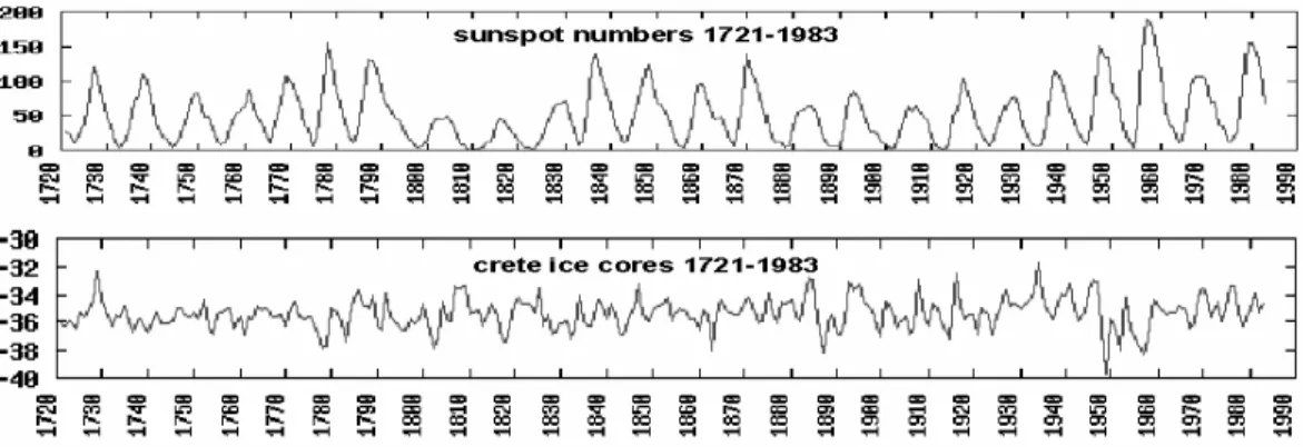
The temperature records are Delta O18/16 values obtained from an ice core drilled at Crete Site-E (71.12 N - 37.32 W), in the center of Greenland. Drilled in 1985, the series covers from 1721 to 1983 (National Climatic Data Center). (Fig.1) The area gets an annual snow accumulation rate of about 20 − 30 g · cm−2. Each year, the accumulation of
winter snow buries the much darker and thinner summer layer, as the warmer temperatures tend to evaporate part of the snow, making more visible the dust particles fallen from long distance winds in late winter/early spring. The layered structure of alternating light and dark bands remains visible even when the weight of the accumulated snow turns it into ice. These bands can be counted by eye. With records a few centuries long and high quality sampling, as with Crete Site-E ice core (eight samples per year), the dating accuracy for yearly data is considered reliable.
The water vapor which becomes snow flakes in Greenland comes from equatorial latitudes. During the long travel, the heavier Oxygen 18 isotope is more easily incorporated into water droplets than the Oxygen 16, a process called Rayleigh fractionation, resulting in a relative increase of the lighter one when reaching the high latitudes. Thus, the Oxygen 18/16 ratio varies as latitude increases, depending also on temperature, cloudiness, and distance to the sea. For a certain location, if general atmospheric circulation conditions remain more or less constant, ground observations show a direct correlation, even if with a small seasonal variability, between the decreasing O18/16 ratio and diminishing air temperatures.
The O18/16 ratio of the ice, expressed as Delta values, is thus a proxy for the air temperatures at the time the snow fell. However, detailed observations show decadal variations on recent data [9] something which points out to the many uncertainties when dealing with climate temperature from ancient times, as the patterns of the general circulation system could have been very different. However, in the case
Fig. 1. Sunspot numbers and Delta O18/16 for the Crete ice core samples in the 1721-1983 time range.
of the data for this paper, such an effect may not have had a strong relevance, as the analyzed time span is relatively short and, also, because our interest is mainly focused on the time-series inner structure and its variations, not on its absolute temperature values.
These temperature data have been analyzed in relationship with the solar activity as expressed by the International Sunspot Number during the same period of time (Fig.1). These, obtained from the Solar Influences Data Analysis Center in Belgium, use present observations and historical records derived from the procedures laid out by Rudolf Wolf in 1849. Sunspot numbers are considered a good proxy of solar activity. Easy to observe, they appear in variable cycles of, roughly, 11 years, or in 22 year cycles if the north-south magnetic polar shift is taken into account. The average lifetime of sunspots is six days, but many last about two days, with the largest ones being visible for weeks and even months. As the Sun makes one rotation at the equator every 25.6 days (but for poles it takes about 36 days), and as we are witnessing only half of the solar surface, the real daily total sunspot number is invisible to us (however, it can now be guessed by Helioseismic Holography, but that information is still not used when counting Sunspot numbers).
III. MULTIVARIATETIMESERIESMODELMINING
The purpose of model mining in complex data coming from heterogeneous, multivariate, time varying processes [16], [17], [18] is to discover dependency models. A model expresses the relationship between values of a previously se-lected time series (the target), and a subset of the past values of the entire set of series. Different classes of functional models could be considered, in particular, a generalized non-linear auto-regressive (AR) model
ST(t) =
F
S1(t − τ1,1), ··· ,S1(t − τ1,p1), S2(t − τ2,1), ··· ,S2(t − τ2,p2), . . . Sn(t − τn,1), ··· ,Sn(t − τn,pn) (1)where ST(t) is the target signal at time t, Siis the i-th time
series, n is the total number of signals, pi is the number of
time lag terms from signal i influencing ST(t), τi,k is the k-th
lag term corresponding to signal i (k ∈ [1, pi]), and
F
is theunknown function describing the process.
The classical approaches in time series consider mostly univariate, homogeneous (real-valued) time series without missing values [1], [13], [12]. Conventional multivariate approaches are complex and have difficulties in handling heterogeneity, imprecision and incompleteness. A hybrid soft-computing algorithm for this kind of problems using heterogeneous neural networks and genetic algorithms was introduced in [16], in the spirit of [11]. It requires the simultaneous determination of: (i) the number of required lags for each series, (ii) the particular lags within each series carrying the dependency information, and (iii) the prediction function. A requirement on function
F
is to minimize a suitable prediction error measure. The procedure is based on: (a) exploration of a subset of the model space with a genetic algorithm, and (b) use of a similarity-based neuro-fuzzy system representation for the unknown prediction functionF
. The process implies a search in the space of neuro-fuzzy networks (Fig.2).Fig. 2. Multivariate Time Series Model Miner System (MVTSMM). The arc (left) is a parallel genetic algorithm evolving populations of similarity-based hybrid neural networks. The binary strings encode dependency patterns for the target signal. For each, a hybrid neural network is constructed and trained with a fast algorithm. The network represents the prediction function, and is applied to an independent test set. The best models are collected.
that an exploration of the structure of the multivariate series can be made, using the mined models as indicator of internal changes within the process. One way of describing the results is by computing the weighted lag importance function whose general form is
L
w(t, τp,q) =∑ card( ˆM) i=1 µ(τp,q, ˆM
i(t)) · f ( ˆM
i(t)) ∑card( ˆi=1 M)f( ˆM
i)(t) (2)where
M
ˆ is the set of discovered models for a given window, card( ˆM
) is its cardinality, ˆM
i(t) ∈ ˆM
is the i-th model found at time t, µ(τp,q, ˆM
i(t)) is the booleanmembership function of lag τp,q ( from Eq.1 ) with respect
to ˆ
M
i(t), and f ( ˆM
i(t)) is a strictly positive model quality measure (fitness) on ˆM
.IV. GENETICPROGRAMMING
Analytic functions are among the most important building blocks for modeling, and are a classical way of expressing knowledge and a long history of usage in science. From a data mining perspective, direct discovery of general analytic functions poses enormous challenges because of the (in principle) infinite size of the search space.
Within computational intelligence, genetic programming techniques aim at evolving computer programs, which ulti-mately are functions. Genetic Programming (GP) introduced in [5] and further elaborated in [6], [7] and [8], is an extension of the Genetic Algorithm. The algorithm starts with a set of randomly created computer programs. This initial population goes through a domain-independent breeding pro-cess over a series of generations. It employs the Darwinian principle of survival of the fittest with operations similar to those occurring naturally, like sexual recombination of entities (crossover), occasional mutation, duplication and gene deletion. A computer program is understood as an entity that receives inputs, performs computations which transform these inputs and produces some output in a finite amount of time. The operations include arithmetic computa-tion (possibly involving many other funccomputa-tions), condicomputa-tionals, iterations, recursions, code reuse and other kinds of informa-tion processing organized into a hierarchy. GP combines the expressive high level symbolic representations of computer programs with the search efficiency of the genetic algorithm. For a given problem, this process often results in a computer program which solves it exactly, or if not, at least provides a fairly good approximation.
There are many approaches to GP leading to a plethora of variants (and implementations) and a discussion about their relative merits, drawbacks and properties is beyond the scope of this paper. One of these GP techniques is the so-called Gene Expression Programming (GEP) [2], [3]. GEP individuals are nonlinear entities of different sizes and shapes (expression trees) encoded as strings of fixed length. For the interplay of the GEP chromosomes and the expression trees (ET), GEP uses an unambiguous translation system to transfer the language of chromosomes into the language of
expression trees and vise versa. The structural organization of GEP chromosomes allows a functional genotype/phenotype relationship, as any modification made in the genome always results in a syntactically correct ET or program. The set of genetic operators applied to GEP chromosomes always produces valid ETs.
The chromosomes in GEP itself are composed of genes structurally organized in a head and a tail [2]. The head contains symbols that represent both functions (elements from a function set F) and terminals (elements from a terminal set T), whereas the tail contains only terminals. Therefore, two different alphabets occur at different regions within a gene. For each problem, the length of the head h is chosen, whereas the length of the tail t is a function of h, and the number of arguments of the function with the largest arity. The length of the tail is evaluated given by t= h(n − 1) + 1. As an evolutionary algorithm GEP defines its own set of crossover, mutation and other operators [3].
V. EXPERIMENTALSETTINGS
The experiments for exploring the bivariate series com-posed of the z-scores (zero-mean, unit-variance) of both the Delta O18 and the Sunspot numbers with the MVTSMM algorithm were made with the parameters shown in Table.V. The series spans the 1721 − 1983 time range (the sampling interval is one year), with a length of 163 points. The number of sliding windows runs was 489 as networks with 3, 4 and 5 number of responsive neurons were explored. The experiments were performed in a distributed computer environment using the Condor system (http://www.cs. wisc.edu/condor/).
TABLE I
SETTINGS FOR THE EXPERIMENTS WITH THEMVTSMMALGORITHM.
General parameters Genetic parameters
maximum lag/series 25 population size 1000
number of number of
responsive neurons 3, 4, 5 generations 50
similarity measure based on
euclidean selection operator tournament distance
model quality RMSE crossover operator single-point
sliding window size 101 crossover prob. 0.6
training set 75% mutation operator bit reversal
validation set 25% mutation prob. 0.01
reproduction prob. 0.1 number of best
chromosomes 300
retained
Three time windows were used for the exploration of local models with Genetic Programming, placed at the beginning, middle and final points of the time-series (mid-window point years of 1795, 1863 and 1933). Some of them cannot reflect the recent climatic anomalies usually associated with human influence. These windows covered the following time ranges: first window: 1746-1845, middle window: 1814-1913, last window: 1884-1983. Within each window, 75% of the ob-servations were used for training and the remaining 25% for
testing the model. Two sets of experiments composed of 500 independent runs each were conducted for all of the three windows previously described, with the genetic programming algorithm parameters shown in Table. V.
TABLE II
GENETIC PROGRAMMING SETTINGS AND GENETIC OPERATORS FOR THE EXPERIMENTS PERFORMED ON THE THREE TIME WINDOWS.
General parameters Genetic parameters
Chromosomes 50 Mutation Rate 0.044
Genes 5 Inversion Rate 0.1
Head Size 15 IS Transposition Rate 0.1
Tail Size 16 RIS Transposition Rate 0.1
Linking Function Addition One-Point
Recombination Rate 0.3
Two-Point
Recombination Rate 0.3
Gene Recombination Rate 0.1 Gene Transposition Rate 0.1
Exp-1 was performed with Root Relative Squared Er-ror (RRSE), whereas Exp-2 used the classical Root Mean Squared Error (RMSE). They are given by
RMSE= r ∑ni=1(Pi− Ti)2 n , RRSE = s ∑ni=1(Pi− Ti)2 ∑ni=1(Ti− T )2 (3) where Piand Tiare the predicted and target values for the
i-th observation respectively. T is the mean of the observed values.
Partially overlapping function sets were chosen for the two rounds of GP experiments in order to change slightly the number and complexity of the functional building blocks for the models. For each rounds 500 GP runs were made, changing the initial population at random. The results were ranked according to their training and test fitness, derived from the corresponding error measures as f itness= 1000 ∗ (1/(1 + error)) (Table.V.).
TABLE III
ERROR MEASURES ANDFUNCTION SETS FOR THE TWO ROUNDS OFGP
EXPERIMENTS.
Exp-1 Exp-3
Error measure RRSE RMSE
+, −,∗,/,x2, x3, +, −,∗,/,xy, ex, ln,
Function Set √,√,e3 x, ln, sin, cos, asin, acos, sin, cos, atan asinh, acosh
VI. RESULTS
A. Multivariate Time Series Model Mining
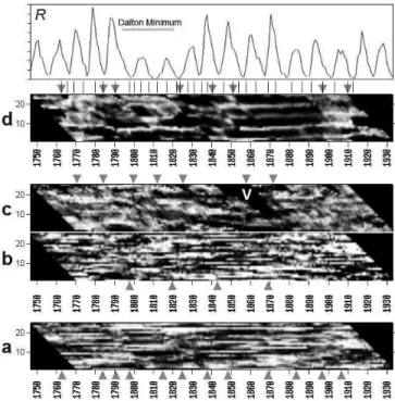
Three independent runs were done (Fig.3): the ice core temperature series (a), the Sunspot series (d), and a join analysis of both of them (b, c), using the temperatures as the target. The image in (c) is the contribution of Sunspot activity to the explanation of the ice core temperature record. Image (b) is what is left of the internal structure of the ice core record when the solar influence is discounted. The horizontal axis is time in years. The vertical axis is time-lags (25, for
this exercise) for each one of the years, visualized by its importance spectra. These have been progressively displaced to the left in order to be placed at the right time.
Fig. 3. Lag importance spectra (Lw(t, τ
p,q) functions) (sheared). Horizontal
axis is time in years, vertical axis is the lag with respect to the current time position: (a): Delta O18/16 Crete (univariate), (b)(c): the bivariate series Delta O18/16 Crete (b) and Sunspot numbers (c). (d): Sunspot numbers (univariate). Top, plot of the International Sunspot Number series for the period. The spectra were sheared 45 degrees to the left in order to get vertical lines as Isochrones.
A common feature of the images is the persistence of particular time-lags running continuously for a number of years. Frequently several bands are interrupted, or begin, at the same time, suggesting packages of years with similar characteristics or behavior. These discontinuities are marked with a gray triangle. Five of the twelve discontinuities in (a) are also exactly present at (d), clearly pointing out to a common timing of the temperature records in Greenland with the solar activity. Comparing (d) and (c) a number of differences can be observed, showing clearly that only part of the Sunspot activity has an influence on temperatures and that it doesn’t follow necessarily the same pattern. The letter V marks a period of time around 1880 with almost no solar influence, in accordance with the low registered solar irradiance for that period.
In (d), apart from the inverted triangles signaling the main blocks of the image, there are also a number of other minor divisions marked by vertical segments. Some of them could perhaps be artifacts due the parameters chosen for the analysis or to poor data quality, as it may be the case for the interruption at 1792, inside a period from 1790-1794 with few observations [15], but most of the rest seem to be related to particular features of the International Sunspot Number (top). A very clear feature of the image is the presence of the Dalton Minimum (1793-1820), a shorter
period than the Maunder Minimum (1645-1715) responsible for the Little Ice Age. The temperatures (a) also register the event, but beginning in 1795-1797 and lasting till 1816, where another event may perhaps be masking the signal: the 1815 eruption of the Tambora (island of Sumbawa, Indonesia) which produced the so known ”Year Without a Summer.”
In Fig.4 each point is the mean of the 300 best networks found. It shows that the fitness is large at the beginning and end of the series, and low in the middle. Since the search strategy is the same in all cases, this behavior suggests the existence of three time intervals along the process with dif-ferent properties (also suggested by the
L
w(t, τp,q)-spectra).
Fig. 4. Mean model quality expressed as f itness= (1000/(1+RMSError)) over the best 300 models computed for each year.
B. Genetic Programming Results
The analytical models corresponding to the 1746-1845 window are given by Eqs.4, for Exp-1 run 099 (RRSE) and Eqs.5, for Exp-3 run120 (RMSE):
δt = sin(k1∗ δt−19) + cos(atan2(e(SSNt−13+(k2∗√SSNt−21)) − SSNt−11)) + sin(sin(sin(k3∗ δt−19))) + δt−19 + sin2(SSNt−23) (4)
where δ is the isotope ratio Delta O18/16, SSN is the sunspot number, the subscript t − i for i ∈ [1, 25] represents the i-th time lag and k1= 0.99888, k2= −4.216797, k3= 0.99522
are constants. δt= asinh(sin(asinh(sin(e(δt−1−(SSNt−11+δt−7))))) ∗ SSN t−1) +cos(cos(asinh((SSNt−10− ((SSNt−11− (k1∗ SSNt−22)) ∗k2)) − SSNt−21) − SSNt−10)) +k3
+asinh(sin(δt−10/k4) + e(sin(SSNt−24)−ln(asinh(SSNt−12+k5))))
+asin(cos(δt−16)) + δt−16
(5) the notation is the same as in Eq.4, and k1= 9.134369,
k2= 8.423248, k3= −6.08489 10−4, k4= 2.236908, k5=
5.55658 are constants.
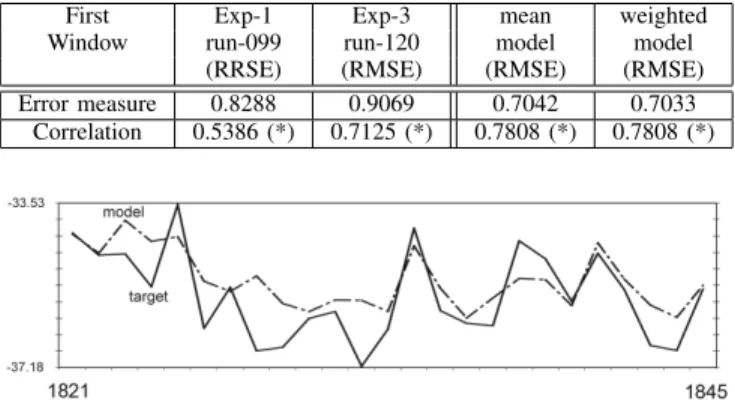
From the individual best models found, two committees of experts (ensemble models) were computed based on: i) their mean, ii) their weighted mean using the fitness derived from their error measures as weights. The main results for the 1746-1845 window are shown in Table.VI-B. The ensemble models improved the individual ones from the point of view of both error and correlation quality (Table.VI-B, Fig.5).
TABLE IV
GENETIC PROGRAMMING MODELS FOR THE1746-1845TIME WINDOW. TEST SET DATA CORRESPONDING TO YEARS1821-1845. SIGNIFICANCE
AT0.05%CONFIDENCE IS INDICATED WITH(*)IN ALL TABLES.
First Exp-1 Exp-3 mean weighted
Window run-099 run-120 model model
(RRSE) (RMSE) (RMSE) (RMSE)
Error measure 0.8288 0.9069 0.7042 0.7033
Correlation 0.5386 (*) 0.7125 (*) 0.7808 (*) 0.7808 (*)
Fig. 5. GP results for the first window: Observed Delta O18/16 series and test set predictions according to the weighted ensemble model.
For the same window, the corresponding analytic models are given by Eqs.4,5. Although these models contain highly nonlinear dependencies, it is interesting to observe that: i) they involve only a small number of variables (6 out of the potential 50) and ii) the three solar sunspot terms are arround those of the solar cycle (11 and 22 years) (Table.VI-B).
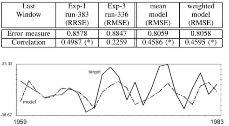
The GP results for the 1814 − 1913 (middle) and the 1884 − 1983 (last) windows are shown in Tables VI-B, VI-B, VI-B and in Figs. 6, 7 respectively. In both cases the behavior and the properties of the ensemble models are similar to those of the 1746 − 1845 window in terms of: i) approximation of the observed Delta O18/16 data, ii) improvement of the model error and correlation measures, iii) sensitivity to only a small number of flagged terms and iv) systematic influence of the solar sunspot events arround the solar cycle (neighborhood of lags 11 and 22).
TABLE V
GENETIC PROGRAMMING MODELS FOR THE1814-1913TIME WINDOW. TEST SET DATA CORRESPONDING TO YEARS1889-1913.
Middle Exp-1 Exp-3 mean weighted
Window run-291 run-319 model model
(RRSE) (RMSE) (RMSE) (RMSE)
Error measure 1.0077 1.0055 0.9577 0.9577
Correlation 0.5253 (*) 0.5447 (*) 0.6107 (*) 0.6107 (*)
Fig. 6. GP results for the middle window: Observed Delta O18/16 series and test set predictions according to the weighted ensemble model..
TABLE VI
GENETIC PROGRAMMING MODELS FOR THE1884-1983TIME WINDOW. TEST SET DATA CORRESPONDING TO YEARS1959-1983.
Last Exp-1 Exp-3 mean weighted
Window run-383 run-336 model model
(RRSE) (RMSE) (RMSE) (RMSE)
Error measure 0.8578 0.8847 0.8059 0.8058
Correlation 0.4987 (*) 0.2259 0.4586 (*) 0.4595 (*)
Fig. 7. GP results for the last window: Observed Delta O18/16 series and test set predictions according to the weighted ensemble model.
VII. CONCLUSIONS
These are very preliminary results emerging from data mining of a very complex problem, which requires further investigation. Although suggestive, the connection of the results with real physical processes remains uncertain in spite of their very promising character. The models obtained are only function approximations which seem to be valid exploration tools for orienting further work. The use of these and other computational techniques on different suspected process-related data (with cross-checking), could provide new and interesting momenta in the global warming issue. The results cannot be used to prove or disprove the possible physical mechanisms behind global warming.
ACKNOWLEDGMENT
The authors would like to thank Robert Orchard from the National Research Council Canada (Institute for Information Technology) for making this research possible.
REFERENCES
[1] G. Box and G. Jenkins, Time Series Analysis, Forecasting and Control, Prentice Hall, 1976.
[2] Ferreira C, “Gene Expression Programming: A New Adaptive Algo-rithm for Problem Solving,” Journal of Complex Systems vol. 13, 2, pp. 87–129, 2001.
[3] Ferreira C, Gene Expression Programming: Mathematical Modeling by an Artificial Intelligence. Springer Verlag, 2006.
[4] IPCC Third Assessment Report. Working Group I: The Scientific Basis. Intergovernmental Panel on Climate Change. WMO, UNEP, 2001. [5] Koza, J. Hierarchical genetic algorithms operating on populations of
computer programs. In Proceedings of the 11th International Joint Con-ference on Artificial Intelligence. San Mateo, CA: Morgan Kaufmann. Vol. I. pp 768–774. 1989
[6] Koza, J. Genetic programming: On the programming of computers by means of natural selection. MIT Press, 1992.
[7] Koza, J. Genetic programming ii: Automatic discovery of reusable programs. MIT Press, 1994.
[8] Koza, J., Andre D., Keane M. Genetic programming III: Darwinian invention and problem solving. Morgan Kaufmann, 1999.
[9] McKenzie, J.A., Anderson, W. T., Teranes, J. L., Bernasconi, S. M. Has the relationship between the oxygen isotopic composition of pre-cipitation and air temperature remained constant over the last century? An example from central Europe. American Geophysical Union, Fall Meeting 2002, abstract #PP52A-0318.
TABLE VII
LAGS CORRESPONDING TO THE VARIABLES COMPOSING THE TWOGP
MODELS OBTAINED FOR THEFIRST WINDOW(1746-1845) (TEST SET).
Delta O18/16 Sunspot Number Lag
Lag Exp-1 Exp-3 Total Exp-1 Exp-3 Total Total
m 099 m 120 m 099 m 120 1 0 1 1 0 1 1 2 2 0 0 0 0 0 0 0 3 0 0 0 0 0 0 0 4 0 0 0 0 0 0 0 5 0 0 0 0 0 0 0 6 0 0 0 0 0 0 0 7 0 7 1 0 0 0 1 8 0 0 0 0 0 0 0 9 0 0 0 0 0 0 0 10 0 10 1 0 10 (2) 2 3 11 0 0 0 11 11 (2) 3 3 12 0 0 0 0 12 1 1 13 0 0 0 13 0 1 1 14 0 0 0 0 0 0 0 15 0 0 0 0 0 0 0 16 0 16 (2) 2 0 0 0 2 17 0 0 0 0 0 0 0 18 0 0 0 0 0 0 0 19 19 (3) 0 3 0 0 0 3 20 0 0 0 0 0 0 0 21 0 0 0 0 21 1 1 22 0 0 0 0 22 1 1 23 0 0 0 23 0 1 1 24 0 0 0 0 24 1 1 25 0 0 0 0 0 0 0 3 5 8 3 9 12 20
[10] Muscheler R., Joosb F., Beer J., Mu¨ller S. A., Vonmoos M., Snowball I. Solar activity during the last 1000 yr inferred from radionuclide records. Quaternary Science Reviews, volume 26, Issues 1-2, pp. 82-97, 2007. [11] V. Petridis and A. Kehagias, Predictive Neural Networks. Applications
to Time Series. Kluver 1998.
[12] A. Pole, M. West, J. Harrison, Applied Bayesian Forecasting and Time Series Analysis., CRC Press, 1994.
[13] G. C.. Reinsel, Elements of Multivariate Time Series Analysis., Springer Verlag, 1993.
[14] Solanki S.K. ,Usoskin I.G., Kromer B., Sch¨ussler M., Beer J. Unusual activity of the Sun during recent decades compared to the previous 11,000 years. Nature, vol. 431, pp. 1084-1087, 2004.
[15] Usoskin I. G., Mursula K. , Kovaltsov G. A. Lost sunspot cycle in the beginning of Dalton minimum: New evidence and consequences. Geophysical Research Letters, vol. 29, 24, pp 2183, 2002.
[16] Vald´es J. J., Time series models discovery with similarity-based neuro-fuzzy networks and evolutionary algorithms. Proceedings of the IEEE world Congress on Computational IntelligenceWCCI2002, vol. 12(5) pp. 2345-2350, 2002.
[17] Vald´es, Barton, A. J. Mining multivariate time series models with soft-computing techniques: A coarse-grained parallel soft-computing approach. Lecture Notes in Computer Science, vol. 2668 LNCS, pp. 259-268. Springer-Verlag, 2003.
[18] Vald´es J. J., Bonham-Carter G., “Time dependent neural network mod-els for detecting changes of state in complex processes: Applications in earth sciences and astronomy.” Neural Networks, 19, pp–196207. 2006 [19] van Dorland R. Scientific Assessment of Solar Induced Climate Change. Report 500102001. The Royal Netherlands Meteorological Institute (KNMI), The Royal Netherlands Institute for Sea Research (NIOZ), 2006.