HAL Id: hal-00409481
https://hal.archives-ouvertes.fr/hal-00409481
Submitted on 8 Jan 2016
HAL is a multi-disciplinary open access
archive for the deposit and dissemination of
sci-entific research documents, whether they are
pub-lished or not. The documents may come from
teaching and research institutions in France or
abroad, or from public or private research centers.
L’archive ouverte pluridisciplinaire HAL, est
destinée au dépôt et à la diffusion de documents
scientifiques de niveau recherche, publiés ou non,
émanant des établissements d’enseignement et de
recherche français ou étrangers, des laboratoires
publics ou privés.
Chemistry Experiment (ACE)
E. Dupuy, K.A. Walker, J. Kar, C.D. Boone, C.T. Mcelroy, P.F. Bernath, J.R.
Drummond, R. Skelton, S.D. Mcleod, R.C. Hughes, et al.
To cite this version:
E. Dupuy, K.A. Walker, J. Kar, C.D. Boone, C.T. Mcelroy, et al.. Validation of ozone measurements
from the Atmospheric Chemistry Experiment (ACE). Atmospheric Chemistry and Physics, European
Geosciences Union, 2009, 9 (2), pp.287-343. �10.5194/acp-9-287-2009�. �hal-00409481�
www.atmos-chem-phys.net/9/287/2009/
© Author(s) 2009. This work is distributed under the Creative Commons Attribution 3.0 License.
Chemistry
and Physics
Validation of ozone measurements from the Atmospheric Chemistry
Experiment (ACE)
E. Dupuy1, K. A. Walker1,2, J. Kar2, C. D. Boone1, C. T. McElroy2,3, P. F. Bernath1,4, J. R. Drummond2,5, R. Skelton1, S. D. McLeod1, R. C. Hughes1, C. R. Nowlan2, D. G. Dufour6, J. Zou2, F. Nichitiu2, K. Strong2, P. Baron7,
R. M. Bevilacqua8, T. Blumenstock9, G. E. Bodeker10, T. Borsdorff11, A. E. Bourassa12, H. Bovensmann13, I. S. Boyd14, A. Bracher13, C. Brogniez15, J. P. Burrows13, V. Catoire16, S. Ceccherini17, S. Chabrillat18, T. Christensen19, M. T. Coffey20, U. Cortesi17, J. Davies3, C. De Clercq18, D. A. Degenstein12, M. De Mazi`ere18, P. Demoulin21, J. Dodion18, B. Firanski22, H. Fischer9, G. Forbes23, L. Froidevaux24, D. Fussen18, P. Gerard18, S. Godin-Beekmann25, F. Goutail26, J. Granville18, D. Griffith27, C. S. Haley28, J. W. Hannigan20, M. H¨opfner9, J. J. Jin29, A. Jones30, N. B. Jones27, K. Jucks31, A. Kagawa7,32, Y. Kasai7, T. E. Kerzenmacher2, A. Kleinb¨ohl13,24, A. R. Klekociuk33, I. Kramer9, H. K ¨ullmann13, J. Kuttippurath13,25, E. Kyr¨ol¨a34, J.-C. Lambert18, N. J. Livesey24, E. J. Llewellyn12, N. D. Lloyd12, E. Mahieu21, G. L. Manney24,35, B. T. Marshall36, J. C. McConnell29,
M. P. McCormick37, I. S. McDermid38, M. McHugh36, C. A. McLinden3, J. Mellqvist30, K. Mizutani7, Y. Murayama7, D. P. Murtagh30, H. Oelhaf9, A. Parrish39, S. V. Petelina12,40, C. Piccolo41, J.-P. Pommereau26, C. E. Randall42,
C. Robert16, C. Roth12, M. Schneider9, C. Senten18, T. Steck9, A. Strandberg30, K. B. Strawbridge22, R. Sussmann11, D. P. J. Swart43, D. W. Tarasick3, J. R. Taylor2, C. T´etard15, L. W. Thomason37, A. M. Thompson44, M. B. Tully45, J. Urban30, F. Vanhellemont18, C. Vigouroux18, T. von Clarmann9, P. von der Gathen46, C. von Savigny13,
J. W. Waters24, J. C. Witte47,48, M. Wolff2, and J. M. Zawodny37
1Department of Chemistry, University of Waterloo, Waterloo, ON, Canada
2Department of Physics, University of Toronto, Toronto, ON, Canada
3Environment Canada, Downsview, ON, Canada
4Department of Chemistry, University of York, Heslington, York, UK
5Department of Physics and Atmospheric Science, Dalhousie University, Halifax, Canada
6Picomole Instruments Inc., Edmonton, AB, Canada
7National Institute of Information and Communications Technology (NICT), Koganei, Tokyo, Japan
8Naval Research Laboratory, Washington, D.C., USA
9Institut f¨ur Meteorologie und Klimaforschung (IMK), Forschungszentrum Karlsruhe (FZK) and Universit¨at Karlsruhe,
Karlsruhe, Germany
10National Institute of Water and Atmospheric Research, Lauder, New Zealand
11Institut f¨ur Meteorologie und Klimaforschung Atmosph¨arische Umweltforschung (IMK-IFU), Forschungszentrum
Karlsruhe, Garmisch-Partenkirchen, Germany
12Institute of Space and Atmospheric Studies, University of Saskatchewan, Saskatoon, SK, Canada
13Institut f¨ur Umweltphysik (IUP), Universit¨at Bremen, Bremen, Germany
14NIWA - Environmental Research Institute, University of Massachusetts, Amherst, MA, USA
15Laboratoire d’Optique Atmosph´erique, CNRS – Universit´e des sciences et technologies de Lille, Villeneuve d’Ascq, France
16Laboratoire de Physique et Chimie de l’Environnement, CNRS – Universit´e d’Orl´eans, Orl´eans, France
17Instituto di Fisica Applicata “N. Carrara” (IFAC) del Consiglio Nazionale delle Ricerche (CNR), Sesto Fiorentino, Italy
18Institut d’A´eronomie Spatiale de Belgique (BIRA-IASB), Bruxelles, Belgium
Correspondence to: K. A. Walker
19Danish Climate Centre, Danish Meteorological Institute, Copenhagen, Denmark
20Earth and Sun Systems Laboratory (ESSL), National Center for Atmospheric Research (NCAR),
Boulder, CO, USA
21Institut d’Astrophysique et de G´eophysique, Universit´e de Li`ege, Li`ege, Belgium
22Science and Technology Branch, Environment Canada, Centre For Atmospheric Research Experiments,
Egbert, ON, Canada
23Environment Canada Sable Island, Dartmouth, Canada
24Jet Propulsion Laboratory (JPL), California Institute of Technology, Pasadena, CA, USA
25CNRS – Service d’A´eronomie (SA), Universit´e Pierre et Marie Curie (UPMC) Paris VI, Paris, France
26CNRS – Service d’A´eronomie (SA), Verri`eres-le-Buisson, France
27School of Chemistry, University of Wollongong, Wollongong, Australia
28Centre for Research in Earth and Space Science, York University, Toronto, ON, Canada
29Department of Earth and Space Science and Engineering, York University, Toronto, ON, Canada
30Department of Radio and Space Science, Chalmers University of Technology, G¨oteborg, Sweden
31Harvard-Smithsonian Center for Astrophysics, Cambridge, MA, USA
32Fujitsu FIP Corporation, Koto, Tokyo, Japan
33Ice, Ocean, Atmosphere and Climate (IOAC) Program, Australian Antarctic Division, Kingston, Australia
34Earth Observation, Finnish Meteorological Institute, Helsinki, Finland
35New Mexico Institute of Mining and Technology, Socorro, NM, USA
36GATS, Inc., Newport News, VA, USA
37NASA Langley Research Center, Atmospheric Sciences Division, Hampton, VA, USA
38Jet Propulsion Laboratory, Table Mountain Facility, Wrightwood, CA, USA
39Department of Astronomy, University of Massachusetts, Amherst, MA, USA
40Department of Physics, La Trobe University, Victoria, Australia
41Atmospheric, Oceanic and Planetary Physics, Oxford University, UK
42Laboratory for Atmospheric and Space Physics, University of Colorado, Boulder, CO, USA
43National Institute for Public Health and the Environment (RIVM), Bilthoven, The Netherlands
44Department of Meteorology, Pennsylvania State University, University Park, PA, USA
45Atmosphere Watch Section, Bureau of Meteorology, Melboune, Vic, Australia
46Alfred Wegener Institute for Polar and Marine Research, Research Unit Potsdam, Germany
47Science Systems and Applications, Inc., Lanham, MD, USA
48NASA Goddard Space Flight Center (GSFC), Greenbelt, MD, USA
Received: 1 November 2007 – Published in Atmos. Chem. Phys. Discuss.: 8 February 2008 Revised: 20 November 2008 – Accepted: 20 November 2008 – Published: 16 January 2009
Abstract. This paper presents extensive bias determina-tion analyses of ozone observadetermina-tions from the Atmospheric Chemistry Experiment (ACE) satellite instruments: the ACE Fourier Transform Spectrometer (ACE-FTS) and the Mea-surement of Aerosol Extinction in the Stratosphere and Tro-posphere Retrieved by Occultation (ACE-MAESTRO) in-strument. Here we compare the latest ozone data products from ACE-FTS and ACE-MAESTRO with coincident ob-servations from nearly 20 satellite-borne, airborne, balloon-borne and ground-based instruments, by analysing volume mixing ratio profiles and partial column densities. The ACE-FTS version 2.2 Ozone Update product reports more ozone than most correlative measurements from the upper tropo-sphere to the lower mesotropo-sphere. At altitude levels from 16 to 44 km, the average values of the mean relative differences are nearly all within +1 to +8%. At higher altitudes (45– 60 km), the ACE-FTS ozone amounts are significantly larger than those of the comparison instruments, with mean rela-tive differences of up to +40% (about +20% on average). For the ACE-MAESTRO version 1.2 ozone data product, mean relative differences are within ±10% (average values within
±6%) between 18 and 40 km for both the sunrise and
sun-set measurements. At higher altitudes (∼35–55 km), sys-tematic biases of opposite sign are found between the ACE-MAESTRO sunrise and sunset observations. While ozone amounts derived from the ACE-MAESTRO sunrise occulta-tion data are often smaller than the coincident observaocculta-tions (with mean relative differences down to −10%), the sunset occultation profiles for ACE-MAESTRO show results that are qualitatively similar to ACE-FTS, indicating a large pos-itive bias (mean relative differences within +10 to +30%) in the 45–55 km altitude range. In contrast, there is no signif-icant systematic difference in bias found for the ACE-FTS sunrise and sunset measurements.
1 Introduction
Ozone is a key molecule in the middle atmosphere because it absorbs solar ultraviolet (UV) radiation and contributes to the radiative balance of the stratosphere. Understanding changes occurring in the distribution of ozone in the atmo-sphere is, therefore, important for studying ozone recovery, climate change and the coupling between these processes (WMO, 2007). To this end, it is important to have continuous high quality measurements of ozone in the stratosphere. Pro-file measurements from satellite-borne instruments provide height-resolved information that can be used to understand changes in ozone concentrations occurring at different alti-tudes. For the past two decades, one of the primary sources for ozone profile information has been satellite-borne instru-ments making solar occultation measureinstru-ments. The solar oc-cultation technique provides self-calibrating measurements of atmospheric absorption spectra with a high signal-to-noise
ratio and good vertical resolution. Thus, to extend this time series of measurements in a consistent way, it is crucial to conduct validation studies that compare the results from new instruments with those from older and more established in-struments.
The newest satellite for solar occultation studies is the At-mospheric Chemistry Experiment (ACE). This Canadian-led satellite mission, also known as SCISAT, was launched on 12 August 2003 (Bernath et al., 2005). There are two instru-ments on-board the spacecraft that provide vertical profiles of ozone and a range of trace gas constituents, as well as temperature and atmospheric extinction due to aerosols. The ACE Fourier Transform Spectrometer (ACE-FTS) (Bernath et al., 2005) measures in the infrared (IR) region of the spectrum and the Measurement of Aerosol Extinction in the Stratosphere and Troposphere Retrieved by Occultation (ACE-MAESTRO) (McElroy et al., 2007) operates in the UV/visible/near-IR. The main objective of the ACE mis-sion is to understand the global-scale chemical and dynam-ical processes which govern the abundance of ozone from the upper troposphere to the lower mesosphere, with an em-phasis on chemistry and dynamics in the Arctic. SCISAT, the platform carrying the ACE-FTS and ACE-MAESTRO, is in a circular low-Earth orbit, with a 74◦ inclination and an altitude of 650 km (Bernath et al., 2005). From this or-bit, the instruments measure up to 15 sunrise (hereinafter SR) and 15 sunset (hereinafter SS) occultations each day. Global coverage of the tropical, mid-latitude and polar re-gions (with the highest sampling in the Arctic and Antarc-tic) is achieved over the course of one year and the ACE measurement latitude pattern repeats each year. When ACE was launched, there were several solar occultation satellite-borne instruments in operation: Stratospheric Aerosol and Gas Experiment (SAGE) II (Mauldin et al., 1985), SAGE III (SAGE ATBD Team, 2002a), HALogen Occultation Exper-iment (HALOE) (Russell et al., 1993), Polar Ozone and Aerosol Measurement (POAM) III (Lucke et al., 1999) and SCanning Imaging Absorption spectroMeter for Atmo-spheric CHartographY (SCIAMACHY) (Bovensmann et al., 1999). The first four instruments only make occultation mea-surements while SCIAMACHY operates in nadir, limb and occultation modes. Between August and December 2005, the SAGE II, SAGE III, HALOE, and POAM III measure-ments ended. Currently, ACE-FTS and ACE-MAESTRO are the only satellite-borne instruments operating exclusively in solar occultation mode, while SCIAMACHY provides oc-cultation measurements in addition to its limb and nadir ob-servations. To be able to extend the long-standing record of observations from the SAGE II, SAGE III, POAM III and HALOE instruments, it is important that the ozone measure-ments provided by ACE-FTS and ACE-MAESTRO be well characterized and their quality thoroughly assessed.
In this paper, we present extensive studies focusing on bias determination for the most recent ozone data products from ACE-FTS (version 2.2 Ozone Update) and ACE-MAESTRO
(version 1.2). The current ozone data are here compared with measurements from satellite-borne instruments as well as ozonesondes and balloon-borne, airborne and ground-based instruments employing different observation tech-niques. Section 2 describes the ACE satellite mission, instru-ments, and the ozone data products. The coincidence crite-ria and the validation methodology are described in Sects. 3 and 4, respectively. The comparisons are organized by in-strument platform in the following two sections, Sect. 5 for the satellites and Sect. 6 for the ozonesondes, balloon-borne, airborne and ground-based instruments. The overall results are summarized and discussed in Sect. 7 and conclusions are given in Sect. 8.
2 The ACE instruments and data products
2.1 ACE-FTS
The primary instrument for the ACE mission, the ACE-FTS, is a successor to the Atmospheric Trace MOlecule Spectroscopy (ATMOS) experiment (Gunson et al., 1996), an infrared FTS that operated during four flights on the Space Shuttle (in 1985, 1992, 1993 and 1994). ACE-FTS
measures high-resolution (0.02 cm−1) atmospheric spectra
between 750 and 4400 cm−1 (2.2–13 µm) (Bernath et al.,
2005). A feedback-controlled pointing mirror is used to tar-get the centre of the Sun and track it during the measure-ments. Typical signal-to-noise ratios are more than 300 from
∼900 to 3700 cm−1. From the 650 km ACE orbit, the instru-ment field-of-view (1.25 mrad) corresponds to a maximum vertical resolution of 3–4 km (Boone et al., 2005). The verti-cal spacing between consecutive 2 s ACE-FTS measurements depends on the satellite’s orbit geometry during the occul-tation and can vary from 1.5–6 km. The altitude coverage of the measurements extends from the cloud tops to ∼100– 150 km. The suntracker used by the ACE instruments cannot operate in the presence of thick clouds in the field-of-view. Therefore the profiles do not extend below cloud top level. The lower altitude limit of the profiles is thus generally 8– 10 km, extending in some cases to 5 km, depending on the presence or absence of clouds.
Vertical profiles of atmospheric parameters, namely tem-perature, pressure and volume mixing ratios (VMRs) of trace constituents, are retrieved from the occultation spectra. This is described in detail in Boone et al. (2005). Briefly, re-trieval parameters are determined simultaneously in a mod-ified global fit approach based on the Levenberg-Marquardt nonlinear least-squares method (see Boone et al., 2005, and references therein). The retrieval process consists of two steps. Knowledge of pressure and temperature is critical for the retrieval of VMR profiles. However, sufficiently accu-rate meteorological data are not available for the complete altitude range of ACE-FTS observations. Therefore, the first step of the retrieval derives atmospheric pressure and
tem-perature profiles directly from the ACE-FTS spectra, using
microwindows containing CO2 spectral lines. During the
second phase of the retrieval process, these profiles are used to calculate synthetic spectra that are compared to the ACE-FTS measured spectra in the global fitting procedure to re-trieve the VMR profiles of the target species. In the current ACE-FTS dataset (version 2.2 with updates for ozone, N2O5, and HDO), profiles are retrieved for more than 30 species us-ing spectroscopic information from the HITRAN 2004 line list (Rothman et al., 2005). First-guess profiles are based on the results of the ATMOS mission. It is important to emphasize that the global fitting approach used here does not use the Optimal Estimation Method, hence does not im-pose constraints based on a priori information. Therefore the retrieval method is not sensitive to the first-guess profiles. Also, averaging kernels are not available for the ACE-FTS retrievals. The altitude range of the ozone retrievals typically extends from ∼10 km to ∼95 km. The final results are pro-vided jointly on the measurement (tangent height) grid and interpolated onto a 1 km grid using a piecewise quadratic method. The latter form is used for all analyses presented in this study. The uncertainties reported in the data files are the statistical fitting errors from the least-squares process and do not include systematic components or parameter correla-tions (Boone et al., 2005). The mean relative fitting errors are lower than 3% between 12 and ∼65 km and typically less than 1.5% around the VMR peak (30–35 km). A detailed er-ror budget including systematic erer-rors is not currently avail-able for the ACE-FTS data products.
Initial validation comparisons for ACE-FTS version 1.0 ozone retrievals have been reported (Walker et al., 2005; Pe-telina et al., 2005a; Fussen et al., 2005; McHugh et al., 2005; Kerzenmacher et al., 2005). Version 2.1 ozone was used in the early validation studies for the Microwave Limb Sounder (MLS) on the Aura satellite (hereafter Aura-MLS) by Froide-vaux et al. (2006). In these earlier ACE-FTS ozone retrievals (up to and including version 2.2), a set of microwindows from two distinct spectral regions (near ∼5 µm and ∼10 µm) was used. Because of apparent discrepancies in the spectro-scopic data for these two regions, the vertical profiles near the stratospheric ozone concentration peak were found to have a consistent low bias of ∼10% in comparisons with other satellite-borne instruments. This was corrected in an update to version 2.2 by removing from the analysis the microwin-dows in the 5 µm spectral region. A consistent set of 37
mi-crowindows around 10 µm (from 985 to 1128 cm−1, with the
addition of one microwindow at 922 cm−1to improve results for the interfering molecule CFC−12) is now used for ozone
retrievals. This O3 data product, “version 2.2 Ozone
Up-date”, is used in the comparisons presented here. These ver-sion 2.2 Ozone Update profiles were used in recent valida-tion studies for Aura-MLS (Froidevaux et al., 2008) and the Michelson Interferometer for Passive Atmospheric Sounding (MIPAS) on Envisat (Cortesi et al., 2007). The agreement with Aura-MLS version 2.2 ozone profiles is within 5% in
the lower stratosphere (with ACE-FTS ozone VMRs consis-tently larger than those of Aura-MLS), but degrades with al-titude with the largest difference in the upper stratosphere (up to ∼25%) (Froidevaux et al., 2008). Relative differences with the MIPAS ESA operational ozone v4.62 data products are within ±10% between 250 and ∼2 hPa (10–42 km) but increase above this range, with ACE-FTS reporting larger VMR values than MIPAS by up to +40% around 0.6 hPa (∼53 km) (Cortesi et al., 2007).
2.2 ACE-MAESTRO
ACE-MAESTRO is a dual-grating diode-array spectropho-tometer that extends the wavelength range of the ACE mea-surements into the near-IR to UV spectral region (McElroy et al., 2007). It records over a nominal range of 400–1010 nm with a spectral resolution of 1.5–2 nm for its solar occulta-tion measurements. The forerunner of the ACE-MAESTRO is the SunPhotoSpectrometer instrument which was used ex-tensively by Environment Canada as part of the NASA ER-2 stratospheric chemistry research program (McElroy, 1995; McElroy et al., 1995). ACE-MAESTRO uses the same sun tracking mirror as the ACE-FTS, receiving ∼7% of the beam collected by the mirror. The ACE-MAESTRO instrument vertical field-of-view is ∼1 km at the limb. The observation tangent altitudes range from the cloud tops to 100 km with a vertical resolution estimated at better than 1.7 km (Kar et al., 2007).
The processing of ACE-MAESTRO version 1.2 occulta-tion data is done in two stages and is described in McEl-roy et al. (2007). In summary, the raw data are converted to wavelength-calibrated spectra, corrected for stray light, dark current and other instrument parameters in the first step. The corrected spectra are then analyzed by a nonlin-ear least-squares spectral fitting code to calculate slant-path column densities for each spectrum, from which vertical
pro-files of O3 and NO2 VMRs are subsequently derived. The
retrieval algorithm does not require any a priori informa-tion or other constraints (McElroy et al., 2007). The inver-sion routine uses the pressure and temperature profiles and tangent heights from the ACE-FTS data analysis to fix the tangent heights for ACE-MAESTRO. Vertical profiles for the trace gases are determined by adjusting an initial guess (high-vertical-resolution model simulation) using a nonlin-ear Chahine relaxation inversion algorithm (see McElroy et al., 2007, and references therein). The final profiles are pro-vided both on the tangent grid and linearly interpolated onto a 0.5 km-spacing vertical grid. As is done for ACE-FTS, the latter profiles are used in the analyses presented in this work. Propagation of the spectral fitting errors in the ozone VMR retrievals yield typical errors of 1–2% between 20 and 40 km and increasing above and below this range. An error bud-get including systematic errors has not been produced for the ACE-MAESTRO ozone product. Averaging kernels are not available for the ACE-MAESTRO retrievals.
As described above, ACE-MAESTRO consists of two spectrophotometers and each can provide vertical VMR pro-files for ozone. Following the previous validation study of Kar et al. (2007), this work presents only the comparisons made with the Visible-Near-IR (VIS) spectrometer ozone data product. The retrieved profiles from the VIS spectrom-eter are in good agreement (mean relative differences within
±10%) with those obtained from the UV spectrometer over
the altitude range where the UV data have good signal-to-noise (∼15–30 km). The VIS profiles provide results over a larger vertical range, necessary for studies in the upper strato-sphere and lower mesostrato-sphere.
The version 1.2 ACE-MAESTRO data products have been compared with SAGE III, POAM III and ozonesonde ob-servations (Kar et al., 2007). Mean relative differences are generally within ±10% from 20–40 km. At higher altitudes, there is a significant bias between the SR observations, for which ACE-MAESTRO reports less ozone than the compar-ison instrument, and the SS observations, which show a large positive bias for ACE-MAESTRO with respect to the coin-cident measurements (of up to +30% around 50 km) (Kar et al., 2007). Direct comparison with the ACE-FTS ver-sion 2.2 Ozone Update profiles was also performed by Kar et al. (2007) for data obtained in the period March 2004– March 2005. The SR comparisons show a low bias of ACE-MAESTRO at most altitudes. The mean relative differences are within ±5% between 22 and 42 km, and increase above and below this range to a maximum value of −30% at 15 and 55 km. For the SS comparisons, the mean relative differences remain globally within ±5% for the Northern Hemisphere occultations, with ACE-MAESTRO VMR values lower than those of ACE-FTS except around 40 km; however, the mean relative differences are larger (within ±10%) for the South-ern Hemisphere observations, with ACE-MAESTRO show-ing less ozone than ACE-FTS below 35 km and more ozone above this altitude (Kar et al., 2007).
3 Temporal and spatial criteria for coincidences
The nominal time period chosen for this study extends over 2.5 years from 21 February 2004 to 31 August 2006. The start date is the first day for which routine, reliable measurements were available for both FTS and ACE-MAESTRO. This time period includes the 2004, 2005, and 2006 Canadian Arctic ACE Validation Campaigns (Kerzen-macher et al., 2005; Walker et al., 2005; Sung et al., 2007; Manney et al., 2008; Fraser et al., 2008; Fu et al., 2008; Sung et al., 2009) and the final period of measurements from the SAGE II, SAGE III, POAM III and HALOE instruments. Based on availability of correlative measurements, this time period has been adjusted for some comparisons.
Common coincidence criteria were used to search for cor-relative observations to compare with FTS and ACE-MAESTRO. In addition to the spatial and temporal criteria
discussed below, it was also required that there were profiles available for both ACE instruments for each coincidence. This provided a consistent distribution of comparisons for ACE-FTS and ACE-MAESTRO. Coincidence criteria can vary widely between different validation studies. The coin-cidence criteria used in this study have been chosen to en-sure a sufficient number of coincidences in all comparisons while trying to limit the scatter resulting from relaxed coin-cidence criteria. For satellite comparisons, a maximum time difference of ±2 h between the ACE observation and the cor-relative measurement, and maximum latitude and longitude differences of ±5◦ and ±10◦, respectively, were generally used. All time differences were calculated using Univer-sal Time (UT). The geographic coincidence criteria corre-spond to maximum distances of ∼600 km at high latitudes and about twice this value near the equator. These distances are of the same order of magnitude as the typical ground-track distance of an ACE occultation (300–600 km). Note that the measurement density is lower at low latitudes be-cause of the high inclination of the ACE orbit and, there-fore, we have significantly fewer coincidences available in the tropics and subtropics. These criteria provide good statis-tics consisting of a few hundred to several thousand events for most satellite-borne instruments. The list of the correla-tive datasets, time periods, number of coincidences and mean values of the distance and of the time, latitude and longitude differences is given in Table 1. For the sparser datasets from ozonesondes and airborne, balloon-borne and ground-based instruments, it is more difficult to find coincidences using the criteria listed above. In those cases, a similar fixed dis-tance criterion was used (800 km for ozonesondes, 500 to 1000 km for other ground-based instruments) but the time criterion was relaxed to ±24 h. This was done in an effort to maximize the number of coincident profiles while at the same time avoiding biases in the atmospheric sampling.
To test the sensitivity of the comparison results to the temporal and geolocation criteria of the correlative measure-ments, we performed comparisons within shorter time peri-ods and smaller geographical regions: typically, comparisons were done for each month of the 2.5-year period and in five latitude bands: four (two in each hemisphere) for mid- and high latitudes (latitudes 30◦–60◦and 60◦–90◦, respectively) and a larger one for the tropics and subtropics (30◦S–30◦N). This analysis was performed for most of the statistical com-parisons with satellite-borne instruments and with ozoneson-des (not shown). In addition, a detailed check of the time series of the mean relative differences, at each ground-based station, was performed for the study presented in Sect. 6.6. These analyses did not show any systematic latitudinal de-pendence of the relative differences or apparent temporal trend in the quality of the ACE observations. We also ana-lyzed the dependence of the relative difference profiles on the distance between the measurement pairs and on observation parameters such as the beta angle for occultation instruments or the solar zenith angle for sun-synchronous measurements
(not shown). This did not reveal significant systematic biases which might have required the use of narrower coincidence criteria. Finally, we did not find any visible latitude bias be-tween the ACE measurements (e.g., ACE latitudes systemat-ically higher or lower than those of the coincident observa-tions) and the correlative instruments (not shown).
It should be noted that broad criteria such as those defined here may result in multiple coincident observations for a par-ticular ACE occultation, for instance when the ACE orbit footprint is close to the satellite ground-track of the correl-ative instrument or when the allowed time difference is large (e.g., 24 h). In such cases, each coincident pair (the same oc-cultation measured by ACE-FTS or ACE-MAESTRO paired with a distinct observation from the comparison instrument) is treated as an independent event, except for the statisti-cal comparisons with ozonesondes (see Sect. 6.5) and Mi-croWave Radiometers (MWRs) (see Sect. 6.9). However, the number of multiple matches did not exceed a few hun-dred for the largest comparison sets (e.g., for comparisons with SABER), with no more than 6–8 distinct comparison measurements coinciding with a single observation from the ACE instruments.
In a first step, the comparisons with all satellite instru-ments (Sect. 5) and with the ozonesondes (Sect. 6.5) were made for ACE-FTS or ACE-MAESTRO SR and SS occul-tations separately. These initial analyses did not show evi-dence for a systematic SR/SS bias in the ACE-FTS dataset. Therefore, averages over all coincidences – without SR/SS separation – are shown for the ACE-FTS analyses in all sec-tions except Sect. 5.1. Since SR/SS differences can be im-portant for intercomparisons between two solar occultation instruments, the results of the comparisons with SAGE II, HALOE, POAM III and SAGE III (Sect. 5.1) are presented separately for both ACE-FTS and the correlative dataset. For the ACE-MAESTRO measurements, there is a known SR/SS bias (Kar et al., 2007). Thus, we present all of the ACE-MAESTRO SR and SS comparisons separately.
Day/night differences in ozone VMR can have an impact on the comparison results in the mesosphere (e.g., Schneider et al., 2005). For the comparisons presented hereafter, we did not routinely use any photochemical model for the ACE measurements to account for these diurnal variations. How-ever, in two cases, a photochemical correction was applied to the correlative data (Sects. 5.4.1 and 5.4.2).
4 Validation methodology
The satellite data used in the following comparisons have vertical resolutions ranging from 0.5 to 5 km, which is the same order of magnitude as those of the ACE instruments (∼3–4 km for FTS and better than 1.7 km for ACE-MAESTRO). Therefore, coincident profiles are linearly in-terpolated onto the ACE vertical grid (with a spacing of 1 km for ACE-FTS or 0.5 km for ACE-MAESTRO) for the
Table 1. Summary of the coincidence characteristics for the instruments (column 1) and data products (column 2) used in the statistical analyses. The full comparison period, latitude range and number of coincidences are presented in columns 3–5. Columns 6–9 give the mean and 1-σ standard deviation for: great circle distance, differences in latitude, longitude and time between the ACE and correlative measurements. For instruments which have multiple retrieval codes, these are noted in parentheses in column 1.
Instrument Data Period Latitude Num. Distance Latitude Longitude Time
version range events [km] diff. [◦] diff. [◦] diff. [min]
SAGE II v6.20 2004/08/09 – 70◦S–66◦N 229 449±234 −1.4±1.9 0.1±5.9 −7±31
2005/05/06
HALOE V19 2004/07/05 – 53◦S–67◦N 49 382±222 0.4±2.2 2.4±5.8 38±46
2005/08/17
POAM III v4 2004/03/16 – 86◦S–63◦S & 376 395±165 0.6±3.1 0.5±5.5 16±53
2005/11/30 55◦N–70◦N
SAGE III v3.0 2004/02/21 – 59◦S–37◦S & 648 328±177 −0.0±2.4 0.3±5.7 −10±31
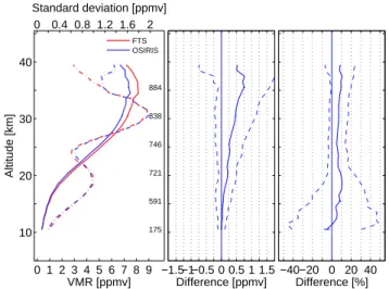
2005/10/09 49◦N–80◦N OSIRIS v3.0 2004/02/24 – 80◦S–86◦N 913 458±231 0.2±2.9 −0.6±5.6 1±66 (York) 2006/08/31 OSIRIS v2.1 2004/03/02 – 79◦S–86◦N 1219 463±229 0.1±2.9 −0.6±5.6 2±67 (SaskMART) 2006/08/05 SMR Chalmers-v2.1 2004/02/21 – 82◦S–82◦N 1161 438±219 0.2±2.8 −0.2±5.7 −1±68 2006/08/31 SABER v1.06 2004/03/02 – 85◦S–85◦N 6210 366±158 −0.1±2.8 −0.2±5.6 0±68 2006/07/31 GOMOS IPF 5.00 2004/04/06 – 72◦S–80◦N 1240 317±122 −0.1±2.0 0.5±41.7 54±438 2005/12/08 MIPAS ESA-v4.62 2004/02/21 – 70◦N–80◦N 138 190±65 −0.5±1.3 −0.4±43.7 68±292 (ESA f.r.)a 2004/03/26 MIPAS ML2PP/5.0 2005/01/27 – 85◦S–86◦N 160 401±225 −0.1±2.8 0.4±5.4 96±210 (ESA r.r.)b 2006/05/04 MIPAS V3O O3 7 2004/02/21 – 30◦N–80◦N 681 276±146c −0.2±1.7c 1.8±9.3c −304±79c (IMK-IAA) 2004/03/26 315±159d −0.2±2.2d −2.2±7.3d 340±98d SCIAMACHY IUP v1.63 2004/03/01 – 80◦S–80◦N 734 339±120 0.6±2.3 −0.1±8.3 −84±233 2004/12/31 Aura-MLS v2.2 2004/09/16 – 80◦S–86◦N 3178 359±156 0.4±2.9 1.5±5.8 12±68 2007/05/23 ASUR n/a 2005/01/24 – 60◦N–70◦N 39 645±225 0.3±3.6 1.7±12.0 208±113 2005/02/07 Ozonesondese n/a 2004/02/22 – 78◦S–83◦N 376 478±210 0.4±3.8 0.1±4.9 8±728 2006/08/03 NDACC n/a 2004/02/21 – 71◦S–83◦N 250 305±135 1.4±1.1 7.7±6.5 302±180 Ozonesondes 2006/08/19 + lidarsf
Eureka DIAL n/a 2004/02/21 – 76◦N–81◦N 10 279±123 −1.7±1.1 −2.4±10.1 417±56
2006/02/23
NDACC v5.0 2004/02/08 – 51◦S–26◦N 43 709±243 −0.3±4.0 0.8±7.0 35±345
MWRsg 2006/10/12
aESA data product for full resolution MIPAS measurements. See text for details. bESA data product for reduced resolution MIPAS measurements. See text for details. cACE vs. MIPAS daytime measurements.
dACE vs. MIPAS nighttime measurements. eStatistical analyses presented in Sect. 6.5. fDetailed NDACC study described in Sect. 6.6. gMWRs at Lauder (45◦
comparison. Tests with other interpolation methods (using quadratic or cubic spline), or by comparing at the actual ACE tangent heights, did not yield any systematic differ-ences. For example, the different interpolation methods gave results within a few percent for the Odin/OSIRIS SaskMART dataset (not shown).
Secondly, for high-resolution measurements such as those from ozonesondes or other instruments measuring in situ, it is necessary to smooth the comparison data. Since averaging kernels are not available for the ACE measurements, alter-native smoothing methods were employed. In this case, two techniques were used, either a smoothing function was ap-plied or an integration method was used.
For most in situ and high-resolution profile comparisons, smoothing (convolution) functions were created for ACE-FTS, consisting of triangular functions of full width at the base equal to 3 km and centered at the tangent heights of each occultation. This value was chosen to account for the smoothing effect of the limited ACE-FTS vertical resolution (∼3–4 km field-of-view), whilst allowing for simplified but valid systematic analysis. Furthermore, it accounts for the vertical spacing of the tangent heights in a retrieved ACE-FTS profile. The spacing varies with altitude (including re-fraction below ∼30 km) and with the beta angle for the oc-cultation (angle between the satellite orbital plane and the Earth-Sun vector). The minimum spacing is about 1.5 km at low altitudes for a high-beta occultation and increases to a maximum value of ∼6 km at mesospheric heights for a low-beta event. High-resolution correlative measurements are convolved with these triangular functions for each ACE tangent height zi: xs(zi) = nhr X j =1 wj(zhrj −zi) · xhr(zhrj ) nhr X j =1 wj(zhrj −zi) , (1)
where xs(zi) is the smoothed mixing ratio for the
high-resolution instrument at tangent height zi, xhr is the VMR
value of the high-resolution profile at altitude zjhr, wj the
associated weight (function of zhrj −zi), and nhr the
num-ber of points from the high-resolution profile found in the
3 km layer centered at zi. The resulting smoothed
pro-file is subsequently interpolated onto the 1 km grid. For
ACE-MAESTRO comparisons, the high-resolution profiles are smoothed by convolution with a Gaussian filter of full width at half-maximum (FWHM) equal to 1.7 km, which is the upper limit for the vertical resolution of the instrument. The smoothed profiles are then interpolated onto the ACE-MAESTRO 0.5 km grid. This smoothing technique was used by Kar et al. (2007).
An alternative method is used in some comparisons with
ozonesondes and lidars (Sect. 6.6). To account for the
higher vertical resolution of the ozonesonde and lidar
mea-surements, these profiles are first integrated to obtain partial columns calculated within layers centered at the ACE mea-surement grid levels (tangent heights). To calculate the par-tial column corresponding to altitude zi, the layer edges are
defined as the mid-points between tangent heights zi−1and zi
(lower limit) and ziand zi+1(upper limit). Then these partial columns are converted to VMR values attributed to the same tangent heights. The resulting profiles are interpolated onto the ACE-FTS (1 km) and ACE-MAESTRO (0.5 km) altitude grids.
Thirdly, for ground-based measurements with lower verti-cal resolution than the ACE instruments (Fourier Transform IR spectrometers (FTIRs) and MWRs), the ACE-FTS and ACE-MAESTRO profiles are smoothed using the averaging kernels calculated during the ground-based retrieval process, following the method of Rodgers and Connor (2003):
xs =xa+A(xACE−xa), (2)
where xACEis the original ACE profile (FTS or
ACE-MAESTRO), xs is the smoothed profile, and xa and A are
the a priori profile and the averaging kernel matrix of the ground-based instrument, respectively.
For the analysis, data are screened to reject either the whole profile or identified low-quality measurements at some altitudes. First, the data from each instrument are filtered ac-cording to the recommendations provided by each calibra-tion/processing team. The specific criteria that were used are described in the appropriate subsections of Sects. 5 and 6. The profiles which do not meet the quality requirements are rejected as a whole. Then, altitude levels for which the stated error represents more than 100% of the profile value, or which exhibit unphysical VMR values – outside of the relatively broad interval of [−10; +20] ppmv – are excluded from the analysis. This generally leads to a lower number of comparison pairs at the lowermost and uppermost altitude levels. Negative VMR values are not systematically rejected as they can be produced by the retrieval process as an arti-fact due to noise in the measurements, especially at altitudes where O3abundance is naturally low. Finally, an initial com-parison step was used to identify and remove erroneous pro-files that were not rejected during the aforementioned anal-ysis (a maximum of 5–6 per comparison set). These gen-eral filtering criteria were applied to all comparisons given in Sects. 5 and 6.
Differences are calculated for each individual pair of pro-files, at the altitude levels where both instruments satisfy the screening criteria described above. The difference at a given altitude z is expressed as
δi(z) =
xACE(z) − xcomp(z)
xref(z)
, (3)
where xACE(z)is the VMR at altitude z for ACE (ACE-FTS
or ACE-MAESTRO), xcomp(z)the corresponding VMR for
xref(z) =1 (abs.)
=xcomp(z) (rel.–gb+o3s)
=(xACE(z) + xcomp(z))/2 (rel.–others)
The first line is the value of xref(z)for absolute difference calculations. The second and third lines give the denomina-tor for calculations of relative differences for the ozoneson-des and the ground-based instruments and for all other com-parisons, respectively. This difference in the relative differ-ence calculation method is based on the assumption that the in situ high-resolution ozonesonde measurements are a good reference for the comparisons, while satellite-borne mea-surements are affected by larger uncertainties and a more logical reference is the average of both instruments VMRs (Randall et al., 2003). There are two exceptions. For the comparisons with the Airborne SUbmillimeter Radiometer
(ASUR, Sect. 6.1), xref(z)=xACE(z) was used. In
com-parisons between ACE and the Global Ozone Monitoring by Occultation of Stars (GOMOS, Sect. 5.4.1) instrument,
xref(z)=xGOMOS(z)was used as the denominator. In
addi-tion, a different calculation methodology has been used for the comparisons with GOMOS. It is explained in detail in Sect. 5.4.1.
The resulting mean differences (absolute or relative) for a complete set of coincident pairs of profiles are calculated as
1(z) = 1 N (z) N (z) X i=1 δi(z), (4)
where N (z) refers to the number of coincidences at altitude
zand δi(z)is the difference (absolute or relative) for the ith
coincident pair calculated using Eq. (3). The mean relative differences are given in percent in the following sections.
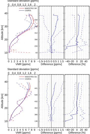
In some cases, notably for ACE-MAESTRO, there may seem to be a discrepancy between the apparent differences given by the mean profiles and the sign of the mean relative differences, or between the signs of the mean absolute and relative differences. The reader is reminded that the mean relative differences are not calculated from the mean VMR profiles but from each pair of coincident profiles (Eq. 3). Thus, the mean relative differences can become negative, even though the mean absolute differences are positive, if some profiles exhibit unusually low VMR values at certain altitude levels or if the VMRs for both instruments are of the same magnitude but of opposite signs (e.g., for the com-parisons between ACE-MAESTRO and OSIRIS SaskMART, Fig. 10).
Finally, as mentioned in Sect. 2, a full error budget includ-ing estimates of the systematic errors is not available for the ACE data products analyzed in this work. Therefore, it is not possible to conduct a full precision validation study. In order to provide the reader with additional information on the significance of the bias and to set an upper limit to the precision of the ACE instruments, we calculate and show the standard deviation of the bias-corrected differences (referred
to as “de-biased standard deviation” hereinafter) and the sta-tistical uncertainty of the mean.
The de-biased standard deviation is a measure of the com-bined precision of the instruments that are being compared (von Clarmann, 2006). It has been used in previous valida-tion studies, for example for POAM III (Randall et al., 2003) or MIPAS (Steck et al., 2007). It is expressed for a given altitude as σ (z) = v u u t 1 N (z) −1 N (z) X i=1 (δi(z) − 1(z))2, (5)
where N (z) refers to the number of coincidences at altitude
z, δi(z)is here the difference (absolute or relative) for the ith
coincident pair calculated using Eq. (3), and 1(z) the mean difference (absolute or relative) calculated from Eq. (4).
The statistical uncertainty of the mean differences (also known as standard error of the mean or SEM) is the quan-tity that allows the significance of the estimated biases to be judged. It is related to the de-biased standard deviation by
SEM(z) = √σ (z)
N (z). (6)
5 Comparisons – satellites
5.1 Solar occultation instruments
5.1.1 SAGE II
SAGE II (Mauldin et al., 1985) was launched in October 1984 aboard the Earth Radiation Budget Satellite (ERBS) and remained operational until August 2005, thus provid-ing a nearly continuous dataset over 21 years. ERBS was in a 610 km altitude circular orbit with an inclination of 56◦. SAGE II performed two occultation measurements per orbit (1 SR and 1 SS), thus sampling two narrow latitude circles each day. Over the course of a month, observations were
recorded with a nearly global coverage between ∼80◦S and
∼80◦N.
The SAGE II dataset comprises profiles of O3, NO2, H2O and aerosol extinction, measured using seven channels cen-tered at wavelengths from 0.385 to 1.02 µm. The ozone re-trievals use data from the center of the Chappuis absorption band measured by the 0.603 µm channel. The retrieval algo-rithm is described in detail by Chu et al. (1989).
Data versions prior to version 6.00 have been the subject of several publications, including an extensive study of ver-sion 5.96 in the first Stratospheric Processes And their Role in Climate assessment report (SPARC, 1998). In 2000, a ma-jor revision of the retrieval algorithm corrected long-standing data issues (version 6.00). Version 6.00 was used in detailed comparisons with HALOE (Morris et al., 2002) and several other instruments (Manney et al., 2001). Subsequent im-provements, versions 6.10 and 6.20, were made and have
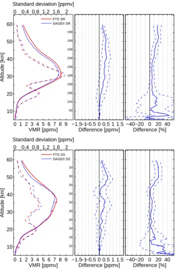
0 1 2 3 4 5 6 7 8 9 10 20 30 40 50 60 VMR [ppmv] Altitude [km] 90 150 199 199 199 199 199 199 199 199 FTS SR SAGEII SR 0 0.4 0.8 1.2 1.6 2 Standard deviation [ppmv] −1.5 −1 −0.5 0 0.5 1 1.5 Difference [ppmv] −40 −20 0 20 40 Difference [%] 0 1 2 3 4 5 6 7 8 9 10 20 30 40 50 60 VMR [ppmv] Altitude [km] 22 29 30 30 30 30 30 30 30 30 FTS SS SAGEII SS 0 0.4 0.8 1.2 1.6 2 Standard deviation [ppmv] −1.5 −1 −0.5 0 0.5 1 1.5 Difference [ppmv] −40 −20 0 20 40 Difference [%]
Fig. 1. Mean profiles and differences for the ACE-FTS − SAGE II coincidences. Results are shown for ACE-FTS SR (top panel) and SS (bottom panel) observations. In each panel: Left: Mean VMR profiles from ACE-FTS and SAGE II (solid lines) and associated 1-σ standard deviations (dot-dashed lines). The standard error – or uncertainty – of the mean (standard deviation divided by the square root of the number of profiles) is shown every 5 km as horizontal error bars on the VMR profiles. Note that in some figures they are smaller than the profile line width and cannot be distinguished. The number of coincident pairs used is given every 5 km. Middle: Mean absolute differences (ACE-FTS−SAGE II) in ppmv (solid line), with corresponding de-biased standard deviations (dashed line), and standard error (uncertainty) of the mean reported as error bars. Right: Mean relative differences in percent (solid line) shown as 2×(ACE-FTS−SAGE II)/(ACE-FTS+SAGE II), de-biased stan-dard deviations of the mean relative differences (dashed line), and standard error (uncertainty) of the mean (error bars).
been extensively validated (Wang et al., 2002; Kar et al., 2002; Iyer et al., 2003; Randall et al., 2003; P. H. Wang et al., 2006). The current version (version 6.20) shows good agreement with correlative measurements within ±5% above
∼18 km. At lower altitudes, the relative differences increase,
with a persistent low bias of −10% or more below ∼10 km (e.g., Borchi et al., 2005; Nazaryan and McCormick, 2005; Froidevaux et al., 2008). This version (v6.20) was used for the comparisons with ACE-FTS and ACE-MAESTRO.
Applying the coincidence criteria (±2 h, ±5◦in latitude
and ±10◦in longitude), we found 229 matches in the period
between August 2004 and early May 2005. Among these, 199 correspond to SR occultations for both instruments, and 30 to both SS observations. The ACE-FTS comparison re-sults are shown in Fig. 1 for the SR/SR (top panel) and the SS/SS (bottom panel) comparisons. ACE-FTS reports con-sistently higher ozone values than SAGE II at all altitudes. The mean relative differences are within +10 to +17% in the range 12–18 km, which is comparable to the low bias of SAGE II ozone values previously reported (e.g., Borchi et al., 2005; P. H. Wang et al., 2006). They are within 0 to +10% between 18 and 42 km for both SR and SS events, with aver-age values of about +5 and +6% for SR and SS, respectively. Above 42 km, both SR and SS comparisons show larger pos-itive differences of up to +20%. Comparisons for SS events yield generally smaller mean relative difference values, no-tably around 12 km and in the range 38–44 km (<3%). Be-low ∼18 km, the de-biased standard deviation of the mean relative differences is large (within 30 to 60% for SR and within 20 to 50% for SS), which is explained by the lower number of coincident pairs and by the large natural variabil-ity of the ozone field at these altitudes. Above 18 km, the de-biased standard deviation of the mean relative differences remains lower than 10% for both SR and SS events up to the top of the comparison range. Note also that there is high consistency shown by the standard deviation of the ACE-FTS and SAGE II mean profiles, which confirms that both instru-ments sounded airmasses with similar variability. Finally, the observed differences are statistically significant as shown by the very small values of the standard errors of the mean.
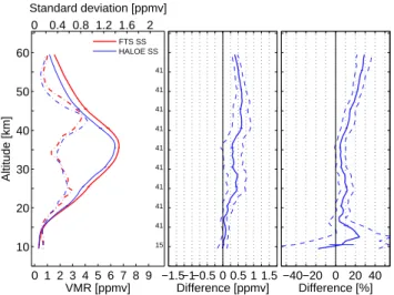
Figure 2 shows the comparisons between the SAGE II and ACE-MAESTRO ozone retrievals for the ACE-MAESTRO SR (top panel) and SS (bottom panel) profiles, respectively. For the SR cases, the agreement is very good between 15 and 55 km with mean relative differences within ±3% through-out, except near 20 km. For the ACE-MAESTRO SS events, the agreement is again quite good (within ±5% between 16 and 45 km), except for a significant positive bias between 45–55 km, reaching a maximum of +17% at 54 km. This is much larger than the SR bias at these altitudes. In con-trast to ACE-FTS, the relatively large standard errors of the mean relative differences for the ACE-MAESTRO compar-isons show that the observed biases are only marginally sig-nificant: below 20 km for both SR and SS events, and in the upper stratosphere for the SS comparisons. The standard de-viation of the mean VMR profiles shows a noticeable scatter of the ACE-MAESTRO VMR values, also reflected in the de-biased standard deviation of the mean absolute and rel-ative differences. These are within 30 to 70% for the SR comparisons and within 10 to 50% for the SS comparisons.
0 1 2 3 4 5 6 7 8 9 10 20 30 40 50 60 VMR [ppmv] Altitude [km] 57 144 187 190 189 192 193 195 195 197 MAESTRO SR SAGEII SR 0 0.4 0.8 1.2 1.6 2 Standard deviation [ppmv] −1.5 −1 −0.5 0 0.5 1 1.5 Difference [ppmv] −40 −20 0 20 40 Difference [%] 0 1 2 3 4 5 6 7 8 9 10 20 30 40 50 60 VMR [ppmv] Altitude [km] 20 29 30 30 30 30 30 30 30 30 MAESTRO SS SAGEII SS 0 0.4 0.8 1.2 1.6 2 Standard deviation [ppmv] −1.5 −1 −0.5 0 0.5 1 1.5 Difference [ppmv] −40 −20 0 20 40 Difference [%]
Fig. 2. Same as Fig. 1, but for the comparisons between ACE-MAESTRO and SAGE II. Top: comparison with ACE-ACE-MAESTRO SR observations; bottom: comparison with ACE-MAESTRO SS observations.
The estimated biases in the stratosphere found for ACE-FTS and ACE-MAESTRO are comparable to these found in previous validation studies for SAGE II. Note also that this analysis provides an incomplete test of biases in the ACE (or SAGE II) datasets since the ACE SR (SS) occultations are all coincident with SAGE II SR (SS) occultations.
5.1.2 UARS/HALOE
The Upper Atmosphere Research Satellite (UARS) (Reber et al., 1993) was deployed from the Space Shuttle Discovery in September 1991. The satellite circled the Earth at an
alti-tude of 585 km with an orbital inclination of 57◦. HALOE
(Russell et al., 1993) remained in operation until November 2005 and performed two occultation measurements per or-bit. A nearly-global latitude range (75–80◦S to 75–80◦N) was sampled in about 36 days.
0 1 2 3 4 5 6 7 8 9 10 20 30 40 50 60 VMR [ppmv] Altitude [km] 15 41 41 41 41 41 41 41 41 41 FTS SS HALOE SS 0 0.4 0.8 1.2 1.6 2 Standard deviation [ppmv] −1.5 −1 −0.5 0 0.5 1 1.5 Difference [ppmv] −40 −20 0 20 40 Difference [%]
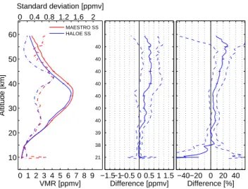
Fig. 3. Same as Fig. 1, but for the comparisons between ACE-FTS and HALOE. Because of the limited number of SR comparisons, results are shown for ACE-FTS SS observations only.
HALOE observations used 8 channels to measure infrared absorption bands between 2.45 and 10.04 µm, providing VMR profiles of trace constituents (including O3, H2O, NO2, and CH4) with a vertical resolution of ∼2 km. O3profiles are retrieved with an onion-peeling scheme from the 9.6 µm channel, which provides an accurate product from the upper troposphere to the mesopause (Russell et al., 1993).
Extensive validation studies have been conducted for pre-vious versions of the HALOE dataset (e.g., for version 17: Br¨uhl et al., 1996; for version 18: Bhatt et al., 1999). The latest version, version 19 (hereinafter V19) has also been
compared to numerous correlative measurements. Good
agreement, to within ∼10%, was found in comparisons with various satellite-borne instruments for the mid-latitudes in November 1994 (Manney et al., 2001). Differences of 4 to 11% were found between HALOE V19 and SAGE II ver-sion 6.10 throughout the stratosphere (Randall et al., 2003). The differences with the POAM III version 3 ozone profiles were typically smaller than 5% and always within ±10% (Randall et al., 2003). Comparisons with the MIPAS IMK-IAA version V3O O3 7 retrievals show a global agreement within 10% in the middle and upper stratosphere (Steck et al.,
2007). The agreement of the HALOE V19 O3profiles with
the most recent release (version 2.2) of the Aura-MLS ozone data product is ∼5% between 68 and 2 hPa (∼20–42 km) but degrades to 15% at 100 and 147 hPa (∼15 and ∼14 km, re-spectively), with Aura-MLS values larger than the HALOE values (Froidevaux et al., 2008). In this study, we use the HALOE V19 ozone retrievals.
In the comparisons, only 49 pairs of coincident profiles
were found using ±2 h, ±5◦ in latitude and ±10◦ in
lon-gitude for the coincidence criteria. As for SAGE II, there are no SR/SS collocations, but only SR/SR and SS/SS events
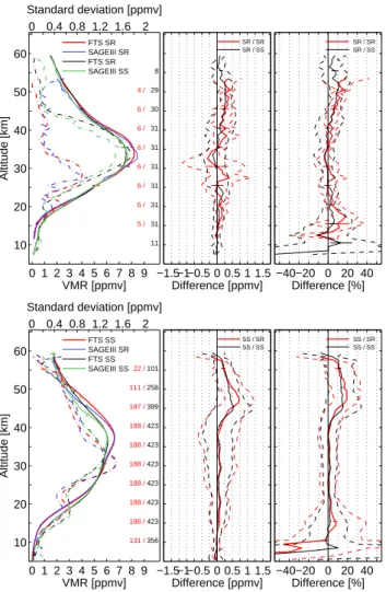
0 1 2 3 4 5 6 7 8 9 10 20 30 40 50 60 VMR [ppmv] Altitude [km] 21 38 39 40 40 40 40 40 40 40 MAESTRO SS HALOE SS 0 0.4 0.8 1.2 1.6 2 Standard deviation [ppmv] −1.5 −1 −0.5 0 0.5 1 1.5 Difference [ppmv] −40 −20 0 20 40 Difference [%]
Fig. 4. Same as Fig. 1, but for the comparisons between ACE-MAESTRO and HALOE. Because of the limited number of SR comparisons, results are shown for ACE-MAESTRO SS observa-tions only.
(respectively 8 and 41 coincidences). In Fig. 3, we present the results for the SS/SS comparisons only, because of the limited number of coincidences for the SR events. The ACE-FTS mixing ratios exhibit a positive bias over most of the alti-tude range. Mean relative differences for the SS comparisons are within +4 to +13% in the range 15–42 km, increasing to about +28% at 60 km. These larger positive mean relative differences are similar to those noted with SAGE II and are a persistent feature in most of the profile comparisons pre-sented in this paper. The de-biased standard deviation of the mean relative differences remains small at all altitudes above
∼17 km (<8% throughout). As for SAGE II, the standard
errors of the mean show that the observed differences are statistically significant.
The ACE-MAESTRO comparisons were also done sep-arately for SR and SS events. As for ACE-FTS, only the comparison between ACE-MAESTRO SS and HALOE SS results is shown (Fig. 4). For this comparison, there is good agreement between 12 km and 40 km, with mean relative dif-ferences within 0 to +10% (+5% on average). The mean rel-ative differences increase thereafter to a maximum of about +27% near 55 km. This is generally similar to the ACE-FTS – HALOE comparison shown above. Contrary to the com-parisons with SAGE II, there is little discrepancy in the stan-dard deviations of the ACE-MAESTRO and HALOE mean VMR profiles, except above 45 km. The de-biased standard deviations of the mean relative differences are larger than those found for ACE-FTS but remain within 10% between 15 and ∼50 km.
5.1.3 POAM III
POAM III (Lucke et al., 1999) was launched in March 1998 onboard the fourth Satellite Pour l’Observation de la Terre (SPOT-4) in a sun-synchronous orbit, with an altitude of 833 km, an inclination of 98.7◦and ascending node crossing at 22:30 (local time). It is a solar occultation instrument able to provide high-resolution (∼1 km) vertical profiles of O3, NO2, H2O and aerosol extinction using nine filter channels from 0.353 to 1.02 µm. POAM III measured in high latitude ranges throughout the year (∼55◦–71◦N and ∼63◦–88◦S), with satellite sunrises in the Northern Hemisphere and satel-lite sunsets in the Southern Hemisphere. POAM III was op-erational from April 1998 to early December 2005.
Briefly, the retrieval algorithm for POAM III consists of a spectral inversion for species separation, followed by the limb (vertical) inversion. Ozone is retrieved primarily from the 0.603 µm channel where the Chappuis absorption domi-nates the total optical depth between 15 and 60 km.
The retrieval and error budget for the version 3 (v3) data products are described in detail in Lumpe et al. (2002). The ozone v3 retrievals have been extensively compared and val-idated using observations from aircraft, balloon and satellite-borne instruments (see Randall et al., 2003, and references therein). They were shown to be highly accurate from 13 to 60 km with a typical agreement of ±5%. A possible slight bias of ∼5% was noted between the SR (Northern Hemi-sphere) and SS (Southern HemiHemi-sphere) profiles, and a high bias (up to 0.1 ppmv) was found below 12 km (Randall et al., 2003). For these comparisons, we use version 4 (here-inafter v4) of the POAM III retrievals. This version was improved to account for problems in the POAM III v3 re-trievals, due in part to unexpected instrument degradation over the course of the mission. Comparative studies simi-lar to those conducted with v3 show that the general conclu-sions of Randall et al. (2003) can be applied to POAM III v4 ozone data (http://eosweb.larc.nasa.gov/PRODOCS/poam3/ documents/poam3 ver4 validation.pdf).
The quality flag implemented for the POAM III v4
O3product (http://eosweb.larc.nasa.gov/PRODOCS/poam3/
documents/poam3 ver4 documentation.pdf) was used for data screening: altitude levels with non-zero values of the quality flag were excluded from the calculations. We used
±2 h, ±5◦ in latitude and ±10◦ in longitude for the coin-cidence search. A total of 376 coincoin-cidences was found in the comparison period, with about 1/3 in the Northern Hemi-sphere (POAM III SR) and the remainder in the Southern Hemisphere (POAM III SS).
Results are shown in Fig. 5 for the ACE-FTS SR (top)
and SS (bottom) occultations. Mean relative differences
are within ±10% (+2 to +5% on average) between ∼12 and ∼42 km for both SR and SS. In particular, the ACE-FTS SS/POAM III SS results show an excellent agreement with mean relative differences within ±3% in the range 23– 41 km and de-biased standard deviation of the mean relative
differences lower than 5%. These are indicative of a good combined precision for these events and therefore imply low random errors for the ACE-FTS retrievals. The largest dif-ferences are found for the ACE-FTS SR/POAM III SS com-parisons (109 coincidences, with mean relative differences within 0 to +13%). Below 16 km, ACE-FTS measures con-sistently less ozone than POAM III, with large mean rela-tive differences corresponding to mean absolute differences of less than 0.1 ppmv. The de-biased standard deviation of the mean relative differences is lower than 8% (SR/SS and SS/SR) and 15% (SR/SR and SS/SS) between about 12 and 42 km. Above 42 km, mean relative differences increase to a maximum of +34% around 60 km. The largest mean rela-tive differences are found for the ACE-FTS SR/POAM III SS events in the range 42–48 km and for the ACE-FTS SS/POAM III SR pairs (∼230 coincidences) above 42 km. In each panel of Fig. 5, a discrepancy in the mean relative differ-ence profiles can be seen, notably at high altitudes. However, when comparing all ACE-FTS SR profiles against POAM III (top panel) and all ACE-FTS SS profiles against POAM III (bottom panel), the resulting differences between the ACE-FTS SR and SS observations are always lower than 1–2% (not shown). Therefore the observed differences should not be interpreted as showing a SR/SS bias of the ACE-FTS data. The ACE-MAESTRO and POAM III comparisons were done by Kar et al. (2007) using measurements from Febru-ary 2004 to September 2005. This slightly shorter compar-ison period did not significantly lower the number of coin-cidences. Therefore, a short summary will be given but the reader is referred to the analysis of Kar et al. (2007) for more information and to their Figs. 6a and 6b for illustration of the results. ACE-MAESTRO SR events show consistently smaller VMRs from 20–50 km when compared to POAM III SR or SS profiles, with mean relative differences within −5 to −15%. The comparison of the ACE-MAESTRO SS pro-files with POAM III yields mean relative differences within
±10% in the altitude range ∼18–40 km, with smallest
val-ues (within ±4% from 20–35 km) for the comparisons of ACE-MAESTRO SS and POAM III SR. Above ∼40 km, the ACE-MAESTRO SS profiles show larger ozone values than POAM III (up to +20% for POAM III SR and +30% for POAM III SS). As for SAGE II or HALOE, the shape of the relative difference profile above ∼45 km for the ACE-MAESTRO SS events is qualitatively similar to the results obtained for ACE-FTS at high altitudes. Here also, the de-biased standard deviation of the mean relative differences is larger than that found for ACE-FTS, within 10 to 25% over the comparison altitude range (18–40 km) (Kar et al., 2007).
5.1.4 SAGE III
SAGE III was an upgraded version of SAGE II and was launched in December 2001 aboard the Russian Meteor-3M satellite. The satellite is in a sun-synchronous orbit at an altitude of 1000 km, with an inclination of 99.3◦and an
as-0 1 2 3 4 5 6 7 8 9 10 20 30 40 50 60 VMR [ppmv] Altitude [km] 4 / 22 / 22 / 22 / 22 / 22 / 22 / 22 / 22 / 22 / 57 96 88 87 109 109 106 106 106 105 FTS SR POAMIII SR FTS SR POAMIII SS 0 0.4 0.8 1.2 1.6 2 Standard deviation [ppmv] −1.5 −1 −0.5 0 0.5 1 1.5 Difference [ppmv] SR / SR SR / SS −40 −20 0 20 40 Difference [%] SR / SR SR / SS 0 1 2 3 4 5 6 7 8 9 10 20 30 40 50 60 VMR [ppmv] Altitude [km] 147 / 227 / 227 / 223 / 224 / 222 / 223 / 223 / 223 / 225 / 12 14 14 14 14 14 14 14 14 14 FTS SS POAMIII SR FTS SS POAMIII SS 0 0.4 0.8 1.2 1.6 2 Standard deviation [ppmv] −1.5 −1 −0.5 0 0.5 1 1.5 Difference [ppmv] SS / SR SS / SS −40 −20 0 20 40 Difference [%] SS / SR SS / SS
Fig. 5. Mean profiles and differences for the ACE-FTS − POAM III coincidences. Results are shown for ACE-FTS SR (top panel) and SS (bottom panel) observations. In each panel: Left: Mean VMR profiles from ACE-FTS and POAM III (solid lines) and associ-ated 1-σ standard deviations (dot-dashed lines). POAM III SR (blue) mean profiles are paired with ACE-FTS (red) mean pro-files and POAM III SS (green) are paired with ACE-FTS (black) mean profiles. The standard error (uncertainty) of the mean is shown every 5 km by error bars on the VMR profiles. The num-ber of coincident pairs used is given every 5 km. Middle: Mean absolute differences (ACE-FTS−POAM III) in ppmv (solid line), with corresponding de-biased standard deviations (dashed line), and standard error (uncertainty) of the mean reported as error bars. The ACE-FTS−POAM III SR and ACE-FTS−POAM III SS differences are shown in red and black, respectively. Right: Mean relative differences in percent (solid line) shown as 2×(ACE-FTS−POAM III)/(ACE-FTS+POAM III), de-biased standard devi-ations of the mean relative differences (dashed line), and standard error (uncertainty) of the mean (error bars). The colour scheme used is the same as that used in the middle panel.
cending node crossing at 09:00 (local time). SAGE III used solar and lunar occultation as well as limb scatter to make measurements in 87 spectral channels (at wavelengths from
0 1 2 3 4 5 6 7 8 9 10 20 30 40 50 60 VMR [ppmv] Altitude [km] 5 / 6 / 6 / 6 / 6 / 6 / 6 / 4 / 11 31 31 31 31 31 31 30 29 8 FTS SR SAGEIII SR FTS SR SAGEIII SS 0 0.4 0.8 1.2 1.6 2 Standard deviation [ppmv] −1.5 −1 −0.5 0 0.5 1 1.5 Difference [ppmv] SR / SR SR / SS −40 −20 0 20 40 Difference [%] SR / SR SR / SS 0 1 2 3 4 5 6 7 8 9 10 20 30 40 50 60 VMR [ppmv] Altitude [km] 131 / 186 / 188 / 188 / 188 / 188 / 188 / 187 / 111 / 22 / 356 423 423 423 423 423 423 399 258 101 FTS SS SAGEIII SR FTS SS SAGEIII SS 0 0.4 0.8 1.2 1.6 2 Standard deviation [ppmv] −1.5 −1 −0.5 0 0.5 1 1.5 Difference [ppmv] SS / SR SS / SS −40 −20 0 20 40 Difference [%] SS / SR SS / SS
Fig. 6. Same as Fig. 5, but for the comparisons between ACE-FTS and SAGE III. Results are shown for ACE-FTS SR observations (top panel) and ACE-FTS SS observations (bottom panel).
280 to 1035 nm) using a grating spectrometer (SAGE ATBD Team, 2002a). The solar occultation observations produced
high-resolution (∼1 km) profiles of O3, NO2, H2O and
aerosol extinction. The SAGE III solar occultation mea-surements occured at high latitudes in the Northern Hemi-sphere (45◦N–80◦N, satellite SS) and at mid-latitudes in the
Southern Hemisphere (60◦S–25◦S, satellite SR). This
pro-vided increased opportunities for measurements coincident with ACE occultation events, particularly in the Northern Hemisphere. SAGE III took measurements from May 2002 through December 2005.
Two different processing algorithms have been used for SAGE III ozone retrievals in the upper troposphere and the stratosphere. One is a SAGE II type (least-squares) algo-rithm using only a few wavelengths and the second one em-ploys a multiple linear regression (MLR) technique to re-trieve ozone number densities from the Chappuis absorp-tion band (SAGE ATBD Team, 2002b). The recent study
of H. J. Wang et al. (2006), using the latest release (ver-sion 3.0) of the retrievals, showed that both products are essentially similar from 15 to 40 km. When compared to correlative measurements, the SAGE II type retrievals pro-vide better precision above 40 km and do not induce artifi-cial hemispheric biases in the upper stratosphere, whereas the MLR retrieval yields slightly better accuracy in the upper tro-posphere/lower stratosphere (UT/LS) region. Comparisons with ozonesondes, SAGE II and HALOE show that the esti-mated precision of SAGE III for the least-squares (SAGE II type) retrieval algorithm is better than 5% between 20 and 40 km and ∼10% at 50 km, and the accuracy is ∼5% down to 17 km. In particular, excellent agreement was found with SAGE II from 15 to 50 km, with ozone values reported by SAGE III systematically larger than those of SAGE II by only 2–3%. Below 17 km, SAGE III ozone VMR values are systematically larger than those of the comparison instru-ments, by 10% at 13 km (H. J. Wang et al., 2006). We use version 3.0 of the ozone data product from the SAGE II type algorithm for the comparisons detailed hereafter.
Of the solar occultation instruments, the most coinci-dences were found with SAGE III (648 events). There is very good overall agreement between ACE-FTS and SAGE III, as shown in Fig. 6. Mean relative differences are within ±6% from 12–42 km (except for the ACE-FTS SR/SAGE III SR results at 17 km) and generally smaller than ±2%. Above 42 km, ACE-FTS reports larger VMRs than SAGE III (by up to +20%). This is consistent with other comparisons pre-sented in this study. There is no significant difference be-tween the ACE-FTS SR and SS comparisons below 42 km. Above this altitude, the SR results show slightly smaller mean relative differences (by −2 to −6%) but are based on a considerably lower number of coincidences. Based on these comparisons, there does not appear to be a systematic SR/SS bias in the ACE-FTS retrievals. The de-biased standard devi-ation of the mean relative differences is within 15% at all al-titudes but often smaller than 6%, a value comparable to the estimated precision of the SAGE III retrievals. This could mean that the ACE-FTS contribution to the combined ran-dom errors of the comparison is very small.
As for POAM III, comparisons of ACE-MAESTRO with SAGE III were conducted by Kar et al. (2007) using nar-rower geographic criteria (maximum distance of 500 km)
and will not be reproduced here. Mean relative
differ-ences within ±5% are found between 15 and ∼40 km for the larger samples (ACE-MAESTRO SS/SAGE III SR and ACE-MAESTRO SS/SAGE III SS). Above this range, the ACE-MAESTRO SS profiles exhibit a large positive bias with mean relative differences of up to +30%, larger than those found for ACE-FTS. The de-biased standard deviation of the mean relative differences is quite large (within 10 to 20%), which suggests that the ACE-MAESTRO spectral fit-ting errors to not entirely account for the random errors of the retrieval. For the ACE-MAESTRO SR measurements, the mean relative differences are consistently within −5 to