Variations of auroral hydrogen emission near substorm onset

(1)

HAL Id: hal-00317815

https://hal.archives-ouvertes.fr/hal-00317815

Submitted on 27 Jul 2005

HAL is a multi-disciplinary open access

archive for the deposit and dissemination of

sci-entific research documents, whether they are

pub-lished or not. The documents may come from

teaching and research institutions in France or

abroad, or from public or private research centers.

L’archive ouverte pluridisciplinaire HAL, est

destinée au dépôt et à la diffusion de documents

scientifiques de niveau recherche, publiés ou non,

émanant des établissements d’enseignement et de

recherche français ou étrangers, des laboratoires

publics ou privés.

onset

L. P. Borovkov, B. V. Kozelov, L. S. Yevlashin, S. A. Chernouss

To cite this version:

L. P. Borovkov, B. V. Kozelov, L. S. Yevlashin, S. A. Chernouss. Variations of auroral hydrogen

emission near substorm onset. Annales Geophysicae, European Geosciences Union, 2005, 23 (5),

pp.1623-1635. �hal-00317815�

(2)

Annales Geophysicae, 23, 1623–1635, 2005 SRef-ID: 1432-0576/ag/2005-23-1623 © European Geosciences Union 2005

Annales

Geophysicae

Variations of auroral hydrogen emission near substorm onset

L. P. Borovkov, B. V. Kozelov, L. S. Yevlashin, and S. A. Chernouss Polar Geophysical Institute, Apatity, Murmansk region, 184209 Russia

Received: 17 February 2005 – Revised: 9 May 2005 – Accepted: 19 May 2005 – Published: 27 July 2005 Part of Special Issue “Atmospheric studies by optical methods”

Abstract. The results of coordinated optical ground-based observations of the auroral substorm on 26 March 2004 in the Kola Peninsula are described. Imaging spectrograph data with high spectral and temporal resolution recorded the Doppler profile of the Hα hydrogen emission; this allows us to estimate the average energy of precipitating protons and the emission intensity of the hydrogen Balmer line. Two different populations of precipitating protons were observed during an auroral substorm. The first of these is associ-ated with a diffuse hydrogen emission that is usually ob-served in the evening sector of the auroral oval and located equatorward of the discrete electron arcs associated with substorm onset. The average energy of the protons during this precipitation was ∼20–35 keV, and the energy flux was

∼3×10−4Joule/m2s. The second proton population was ob-served 1–2 min after the breakup during 4–5 min of the ex-pansion phase of substorm into the zone of bright, discrete auroral structures (N-S arcs). The average energy of the pro-tons in this population was ∼60 keV, and the energy flux was

∼2.2×10−3Joule/m2s. The observed spatial structure of hy-drogen emission is additional evidence of the higher energy of precipitated protons in the second population, relative to the protons in the diffuse aurora. We believe that the most probable mechanism of precipitation of the second popula-tion protons was pitch-angle scattering of particles due to non-adiabatic motion in the region of local dipolarization near the equatorial plane.

Keywords. Auroral ionosphere; Particle precipitation; Storms and substorms

1 Introduction

The hydrogen Balmer lines of Hα (656.3 nm) and Hβ (486.1 nm) were first identified in aurora spectra in Norway (Vegard, 1939). Doppler broadening of the line profiles in-dicated their extraterrestrial origin. More extensive studies

Correspondence to: B. V. Kozelov

(kozelov@pgi.kolasc.net.ru)

of the hydrogen emissions started during the International Geophysical Year (IGY). Almost simultaneously, observa-tions of hydrogen emissions drew the interest of many re-searchers over the world: the USA, Canada, Sweden, Nor-way, Japan and some other countries (see review in Eather (1967)). In the Soviet Union, the pioneering studies of hy-drogen emissions were published by Galperin (1959) and Yevlashin (1961). During next four decades, numerous stud-ies featured the relationship of hydrogen emissions with var-ious forms and types of auroras, latitudinal and longitudinal expansion of the hydrogen emission zone, dependence of hy-drogen emissions on magnetic activity, and the relationship with ionospheric ionization, riometric absorption and ULF-emission, radio reflections from auroras. There the altitude of hydrogen emissions was estimated using sounding rock-ets and the observation of the absolute values of Hα and Hβ intensity was performed, as well as measurements of the Balmer decrement, emission fluctuations and, finally, the re-lationship of hydrogen emissions to auroral breakup and sub-storms in general (see a review by Yevlashin (2000)).

The main patterns of substorm development in proton auroras were described already in the 1970s in a few pa-pers (Montbriand, 1971; Fukunishi, 1975; Yevlashin and Yevlashina, 1980). If one carefully compares results of these and others papers, one can conclude that they all coincide qualitatively in their basic aspects. So, at the growth phase of substorm in the evening, the proton aurora is found to be at lower latitudes than the discrete arcs of the electron aurora, whereas the situation is opposite in the recovery stage in the morning hours. These conclusions have been supported by statistics (Hardy et al., 1991).

As far as the expansion phase is concerned, some impor-tant quantitative differences can be found. In the pattern by Fukunishi, the enhancement of proton luminosity bright-ness is mentioned; by contrast, the paper by Yevlashin and Yevlashina reports the general decrease of proton aurora in-tensity, while the paper by Montbriand draws attention to a flare of proton aurora at the initial moment of the expan-sion phase with its subsequent decrease down to the values less than ones at the growth phase. The possible reasons

(3)

of the differences were, first, the different techniques used for registration of hydrogen emissions (and therefore, for ex-ample, different exposure time) and secondly, difficulties in the interpretation of experimental data, due to strong inten-sification of electron-excited emissions (N21PG and

Vegard-Kaplan bands), that blend the hydrogen spectral lines dur-ing the expansion phase of substorm (Gattdur-inger and Vallance Jones, 1974).

Extensive studies of substorm events during the last two decades have revealed the important role of ions fluxes in the development of instabilities associated with the expansion phase (Delcourt et al., 1994, 1996). The significant varia-tions of proton fluxes found by satellites in the zone of sub-storm expansion, both near magnetic equator (Sauvaud and Winckler, 1980; Kozelova et al., 2004) and at low altitudes (Sergeev and Kubyshkina, 1996), also attract one’s attention. Despite the great achievements of satellite techniques, the di-rect observation of proton fluxes in various magnetospheric domains is usually lost in the space-time ambiguity associ-ated with satellite data. Therefore, the development of opti-cal observations, both ground and satellite, is continuing (see review in Lanchester et al. (2003)). However, the dynam-ics of precipitated proton fluxes and the resulting hydrogen emissions during the late growth and early expansion phases of the substorm are not completely understood.

Using global observations of electron and proton pro-duced auroras observed by IMAGE satellite FUV instru-ments, Mende et al. (2001) concluded that the peak inten-sity of the proton aurora did not change substantially dur-ing substorms. They found that the initial brightendur-ing of the substorm was embedded in proton precipitation, which coincides with the results of Samson et al. (1992). G´erard et al. (2004) supports the results by large statistics. As the electron surge expands poleward it leaves the protons behind. Deehr and Lummerzheim (2001), while using a combination of a high sensitivity all-sky imager and meridian scanning photometers, studied emission parameters in 33 auroral sub-storms in 1992 with proton auroras at Alaska stations. They do not support the argument that the substorm onset begins from within the proton precipitation, but the discovery of the soft electron pulse during “auroral fading” does support theories requiring a pulse of Alfv´en speed electrons. Taka-hashi and Fukunishi (2001) studied auroral breakup events at Syowa station, Antarctica for 35 events of auroral substorms during the period of 1990–1993. The authors believe that at the poleward boundary of auroral bulge the Doppler shift of hydrogen line is quite large, while the maximum intensity of hydrogen emission is observed somewhat equatorward of the leading edge. These facts imply that precipitating protons with higher energies and highly field-aligned pitch angles are produced at the poleward boundary through a plasma injec-tion process in the magnetosphere.

The goal of this paper is a detailed study of the proton precipitation during late growth and early expansion phases of an auroral substorm on 26 March 2004, using the data of coordinated optical ground-based observations in the Kola Peninsula. In addition to the usual observatory equipment

(all-sky TV camera and scanning photometer), a special imaging spectrograph with high spectral and temporal res-olution was used. The data from this device allows us to esti-mate variations of the energy of precipitating proton flux and the hydrogen emission intensity, using the Doppler profile of the auroral Hα emission during the event. An interpretation of optical observations, as well as any indirect method of di-agnostics, is usually based on a theoretical model.

Our estimations of the proton-hydrogen flux parameters are based on the results of simulations of the Doppler-shifted hydrogen line profiles using the Monte-Carlo method (Kozelov, 1993, 1994). The simplified model from Kozelov et al. (1995), based on results of detailed Monte-Carlo trans-port modeling, is used to calculate the spatial structure of the Hα luminosity resulting from such precipitation, for different values of precipitated proton flux parameters. The observed spatial structure of the Hα luminosity supports our conclu-sion about the characteristic energy of proton precipitation before and after substorm onset. Relations between the dy-namics of proton flux observed during the event of interest and the protons’ motion in the region of local dipolarization near the equatorial plane are discussed.

2 Equipment

This study is based on observations provided by the Polar Geophysical Institute at two points: Lovozero observatory (67.97 N, 35.02 E) and Apatity station (67.58 N, 33.31 E). Positions of the observation points are shown on the map in Fig. 1a. During the evening of 26 March 2004, two opti-cal devices were operating at Lovozero observatory: TV All-Sky Camera (TVASC) and Scanning Photometer (SP). The TVASC observed the aurora in “white” light with a broad maximum at blue-green wavelengths. The TV data were recorded by a VHS recorder in a PAL video system, at 25 images per second. The TV data were also digitized using an Acorp TV-Capture plate with an output resolution of 5 images per second, 320×288 pixels, 8 bits per pixel.

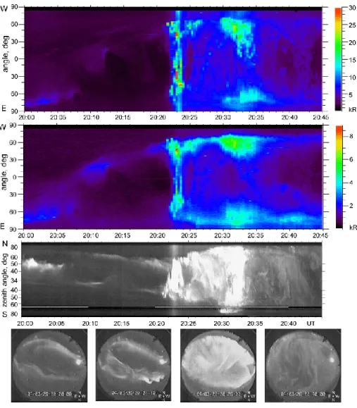
The Scanning Photometer (SP) was scanning approxi-mately in the magnetic east-west direction and monitoring auroral emissions at the wavelengths 427.8 nm (N+₂ 1NG), 557.7 nm (OI) and 630.0 nm (OI). The SP was calibrated by calibration lamp TRS-28-50, with an estimated discrepancy of emission intensity in the 630.0-nm channel of 25%. The trajectory of SP scans in the field of view of the TVASC is shown in Fig. 1b. The magnetometer and riometer at Lovozero observatory was also available to monitor the geo-physical environment.

During the evening of 26 March 2004, at the Apatity station, spectrograph observations of auroras were provided by a special device consisting of an imaging spectrograph SpectraPro 306, made by Acton Research Corp. and an intensified CCD camera IpentaMax, made by Princeton Instruments. The specifications of the spectrograph and CCD camera are the following:

(4)

L. P. Borovkov et al.: Variations of auroral hydrogen emission near substorm onset 1625

Fig. 1. Geometry of observations: (a) observation points; (b) fields of view for optical devices.

Spectrograph SpectraPro 306

– Optical design: Imaging Czerny-Turner with polished aspherical mirrors

– Focal length: 300 mm

– Aperture Ratio: f/4

– Grating with profiled grooves, 1200 gr/mm, 68×68 mm

– Resolution: 0.1 nm at 435.8 nm with 100 µm entrance slit

– Dispersion: 2.7 nm/mm

– Focal plane size: 27 mm wide×14 mm high

– Free spectral interval ∼25 nm with IPentamax camera.

Fig. 2. Schematic of the spectrograph SpectraPro 306 with CCD camera IpentaMax.

CCD camera IpentaMax

– Thermoelectrically cooled CCD matrix 512×1024, 15×15 µm pixels with frame transfer

– Microchannel image intensifier fiber-optically coupled to CCD

– 12 bits 5 MHz ADC converter

– Dark current ∼20 electrons pix−1s−1at −20◦C – Exposure range 50 µs to 23 h

– Computer controls camera and acquires data via high speed serial connection.

The CCD sensor was cooled up to −45◦_{C to reduce the noise}

level. The resulting mean dark charge for the 10-s exposition was about 4 units of the device ADC (Analog to Digit Con-verter). The device is mounted by gimbal to the ceiling and obtains emissions through a plexiglass dome. The schematic view of the device is presented in Fig. 2. We can tilt the device’s optical axis up to 45 deg relative to the vertical di-rection in 2 orthogonal planes. In addition, it is possible to turn the device (and the entrance slit) relative to the optical axis in any direction. With a Nikkor fisheye lens, the full aperture of the device is ∼80×1 deg. We control the spectro-graph and camera with our own original software, using the

(5)

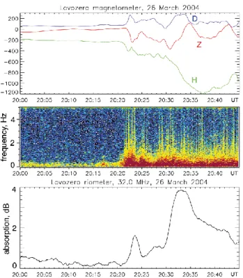
Fig. 3. Substorm event of 26 March 2004: (a) magnetogram at Lovozero observatory; (b) Lovozero magnetometer spectrogram (Y component); (c) riometric absorption observed by Lovozero riome-ter.

low level programming possibilities of the software obtained with both instruments.

The field of view of the spectrograph is shown in Fig. 1b. The SP scan crosses the spectrograph’s field of view (see point 2 in Fig. 1b), and this allows us to calibrate the spec-trograph sensitivity relative to a 630.0-nm channel of the SP using the 636.4-nm emission line. According to Chamberlain (1961) the ratio of these emissions is approximately equal to 3. For calibration we used the diffuse auroral emissions of 630.0 nm in the range 0.3–2.5 kR.

3 Observations

For a detailed study we selected the interval 20:00–20:45 UT, on 26 March 2004. The observations are presented in Figs. 3–5. Figure 3 shows three components of the geomag-netic field, maggeomag-netic pulsations and riometric absorption ob-tained at Lovozero observatory. Figure 4 illustrates the re-sults of the optical observation by the SP and the TVASC at the same points.

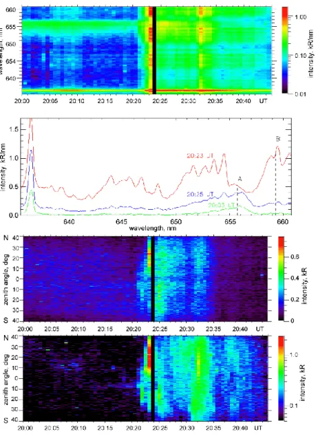
Figure 5 contains the spectrograph data from Apatity sta-tion. There is a gap in the data for ∼30 s from 20:23:35 UT to 20:24:05 UT, due to file saving. The data has both spec-trometric and spatial information about the aurora luminos-ity. The time exposure of the spectrograph data was ∼10 s. Under quite, pre-breakup conditions, the mean signal level at Hα profile maximum was ∼4 units of ADC (Analog to

Digit Converter), that means the signal-to-noise ratio at raw data was ∼1. The top plate of Fig. 5 presents an evolution of the auroral spectrum in the spectral region from 635.5 to 661.0 nm. By summing 3 frames of spectral images and tak-ing an average of 100 rows of image, we improve the signal-to-noise ratio by

√

3 ∗ 100≈17.3 times. So, the statistical error in the data is less than 6%. The averaged rows in the spectral image corresponds to the range of view angles from zenith to ∼18 northward degrees, marked in Fig. 1b by the number “1”.

The shape of the spectrum at several important moments is shown in the second plate. Two spectral regions are marked at the spectrum with “A” and “B”. The spectral region of 655.7–656.2 nm is mainly filled with the Doppler-shifted Hα hydrogen line, however, some contribution from emissions of atmospheric species is also possible, especially for strong electron precipitation (Gattinger and Vallance Jones, 1974). The second spectral region is formed only by atmospheric emissions, mostly by a line from N21PG system. Spatial

evolution of the auroral luminosity in these spectral regions is illustrated in two plates with keograms in the north-south direction.

The interval under consideration started from the late growth phase of the substorm. According to TVASC data, in the beginning of the interval, an active bright arc was lo-cated on the north side of the all-sky image (∼130 km from Lovozero), and a slow diffuse arc was observed near the zenith; see Fig. 1b. During the next 20 min there was a slow evolution of the arc system: motion of the first arc to the zenith of TVASC, occurrence of a new arc at the previ-ous position of the first arc, intensification of the zenith arc (∼20:07 UT), and then dissipation at ∼20:12 UT and the next intensification at ∼20:17 UT. All this activity was ac-companied by large-scale motion of the aurora in the south-ward direction; this is a normal feature for the growth phase of the substorm (Akasofu, 1968). However, remarkable vari-ations in the magnetic field and riometer absorption were not observed; see Fig. 3. During this interval, the Hα hydrogen line with Doppler shift to the blue side was observed at all view angles of spectrograph (see green spectra in Fig. 5b), that indicates a wide zone of the proton precipitation. Fig-ure 5c shows that in the northern part of the view angles the intensity of the hydrogen line was gradually decreasing, but in the southern part, it was increasing. Therefore, we can deduce that the proton precipitation zone was moving towards the south, too. The estimated width of the diffuse zone of the hydrogen emission was ∼200 km. The slow elec-tron arc mentioned above was also the spectrograph’s field of view. The evolution of the discrete arc intensity is shown by N21PG emission (659.3–659.8 nm emission band, marked in

Fig. 5b as “B”); see Fig. 5d. However, the arc had no influ-ence on the spectral region of blue-shifted Hα emission; see Fig. 5c.

An intensification of the near-zenith arc, which started from 20:21 UT simultaneously with the increase of the mag-netic pulsations (Fig. 3b), developed into the breakup ob-served at 20:22 UT. The expansion phase of the substorm

(6)

Fig. 4. Optical observations at Lovozero: (a) data of east-west Scanning Photometer (SP) in 427.8 nm emission; (b) SP data in 630.0 nm emission; (c) TV keogram in north-south direction (see Fig. 1); (d) TV all-sky images at several moments.

proceeded in two steps shown by a drop in the H-component of the magnetic field (Fig. 3a), indicating the development of the magnetosphere-ionosphere current system. Each drop corresponds to an increase in riometer absorption (Fig. 3c) and an intensification of optical aurora. These two steps cor-responded to the aurora expansion in the north-south direc-tion and are obvious in the TVASC keogram, Fig. 4. The longitude region of the auroral event was located between the positions of two LANL satellites, 01A and 02A. The satellite data (not presented here) show the appearance of two injec-tions of high-energy particles at ∼20:21 UT and ∼20:28 UT. During the expansion phase of the substorm, the Hα hy-drogen line was blended with very strong emissions of the excited atmospheric species (see red spectra in Fig. 5b), mainly N21PG (Gattinger and Vallance Jones, 1974).

There-fore, we can deduce that strong electron precipitation oc-curred. However, after the first intensification of the electron precipitation during several minutes (20:24–20:29 UT) one can also see an increased hydrogen emission (see blue

spec-tra in Fig. 5b). This intensification of the hydrogen emis-sion corresponds to several patches at northward view angles in spatial distribution in Fig. 5c. This structure is absent in Fig. 5d, therefore, this is not an intensification of the blended emissions excited by electron precipitation. Simultaneously with this intensification of the hydrogen emission, N-S ori-ented arcs appeared on the north side of TVASC images; see Fig. 4, image at 20:26:00 UT. After 20:35 UT the hydrogen emission is absent, all other aurora emissions are decreasing, TVASC images were filled with pulsating aurora structures, which is a normal picture for the recovery phase of substorm. During the event of interest we observed two “popula-tions” of precipitated protons. One of them produced a diffuse hydrogen zone during the preliminary phase of the substorm. Another one was observed during the expansion phase; it had a more sharp and active precipitation region. What difference exists between these populations and the mechanisms of their precipitation? To answer the question in the next sections we will try to separate the hydrogen

(7)

Fig. 5. Spectrograph data at Apatity: (a) evolution of spectrum averaged in 0◦-18◦North zenith angles (the region marked by “1” in Fig. 1); (b) spectra at several moments; (c) north-south keogram in “A” emission band (655.7–656.2 nm, mainly Doppler-shifted Hα); (d) north-south keogram in “B” emission band (659.3–659.8 nm, N₂1PG).

emission from blended spectra and to estimate the energy of precipitated protons.

4 Separation of the Hα profile

The main problem for detection of the Hα Doppler-shifted line is blending by numerous other emissions (Gattinger and Vallance Jones, 1974). Theoretical models of the auroral emission spectrum are not available with the quality which would allow one to separate the shape of the Hα line from the experimental spectrum with sufficient precision. Therefore, here we use a semiempirical method based on experimental data itself.

We will assume that the spectrum of all emissions in the range of 640–660 nm, excluding Hα, has the same shape,

and that relations between intensities of different lines in the range do not depend on characteristics of incoming parti-cle flux. This assumption has a theoretical substantiation. The auroral spectrum near Hα during nighttime is formed mainly by lines of a 1-PG band emitted from the B35gstate

of molecular nitrogen. The efficiency (so-called “energetic cost”) of the state excitation by electrons does not depend on the electron energy of the auroral range and it does not depend on altitude (from 100 to 200 km); see Sergienko and Ivanov (1993). The excitation rate of the B35g state of N2

in a volume unit is directly proportional to the energy depo-sition rate by electron flux in this volume unit. Integration along the line of sight does not change this proportion, inde-pendent of the geometry (shape) of the electron precipitation and the direction of the line of sight. The lifetime of the B35g state is too short to have a remarkable quenching at

(8)

Fig. 6. Average spectrum of electron excited lines in the spectral range of 636.0–661.0 nm.

Fig. 7. Evolution of separated Hα hydrogen emission: (a) spectra after removing the background emissions; (b) integral intensity in the range of 651–657 nm.

the auroral altitudes (Kirillov, 2004). So, all these excita-tions of the state lead to emission of 1-PG band lines. The remaining problem is relations between intensities of differ-ent rotational lines. Ordinarily, these relations must depend on the local atmospheric temperature (Gattinger and Val-lance Jones, 1974). The temperature changes dramatically in changing precipitation energy. However, for weak incoming fluxes of electrons and protons, we make the assumption that the temperature dependence of the spectrum shape is possi-ble weak.

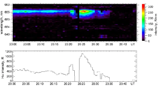
To obtain the shape of blended emission spectrum, we cal-culate an average normalized spectrum during the time inter-val 20:38–20:45 UT, when the shifted Hα emission was ab-sent. The integral intensity in 642–647 nm has been used for normalization. The average normalized spectrum is shown in Fig. 6. Then, using the normalized spectrum and integral intensity in 642–647 nm for each spectrum in the considered event in order to obtain the magnitude, we then remove the blended emissions from spectrograph data. The results are presented in Fig. 7a. One can clearly see the Hα emission line in spectra from 20:00 to 20:21 UT, where blended emis-sions were fully removed in the spectra.

However, the residual emissions are clearly seen during an interval of strong electron precipitation, accompanied by

increased riometer absorption. Obviously, this is a result of dependencies not taken into account in our separation pro-cedure. It is interesting that after removal of the blending emissions, the Hα emission is practically absent in the spec-trum at 20:23 UT, which corresponds to the strongest aurora emission during the breakup of the aurora arc.

The total intensity of the Hα emission has been estimated by the integration of the spectra from Fig. 7a. Figure 7b illus-trates the temporal evolution of the integral intensity of the separated Hα spectra in the range of 651–657 nm.

5 Estimation of proton energy

Estimations of the proton-hydrogen flux parameters are based on the results of simulations of the Doppler-shifted hydrogen line profiles using the Monte-Carlo method. The algorithm was successfully validated in Kozelov (1994) by comparison with particle data from a rocket campaign by Søraas (1974). The algorithm takes into account the 3-component atmosphere (N2, O, O2) (Hedin, 1987), the

influence of the Earth’s dipolar magnetic field (Kozelov, 1993) and the collisional angle scattering based on differen-tial cross sections evaluated from laboratory measurements (Fleischmann et al., 1967, 1974; Newman et al., 1986;

(9)

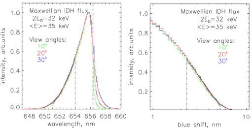
Fig. 8. Simulated Hα profiles for view angle relative to the magnetic field line direction: green − 10◦; red − 20◦; blue − 30◦. Black solid line is the least-squares fit of Eq. (1), dash-dotted line marks the fit range, dashed line is a position of non-shifted Hα line. (a) full profiles; (b) blue-shifted wing in log-linear coordinates.

Van Zyl et al., 1978; Gao et al., 1990). The formalism of the calculation of the Doppler profiles from transport algo-rithms is well-known; see, for example, Lorentzen et al. (1998). Here we only note that our interest is the high-energy (>10 keV) proton precipitation; therefore, we assume that the proton fluxes are isotropic in the downward hemisphere (IDH) in pitch-angle distribution and have a Maxwellian en-ergy distribution. Figure 8 presents an example of the sim-ulated profiles of the hydrogen line for precipitated proton flux having a Maxwellian energy distribution with a charac-teristic energy of E0=16 keV, so the average energy of

parti-cles in precipitated flux is <E>=2 E0=32 keV. The isotropic

pitch-angle distribution results in the independence of the blue wing of the profile on the view angle relative to the mag-netic field line direction in the range from 0◦to 30◦.

As we have noted above, the Doppler-shift of the maxi-mum of the hydrogen line profile is not a good characteris-tic of the energy of precipitated proton flux. The blue wing of the profile is the most informative region to characterize the flux energy. For precipitation of the monoenergetic pro-ton flux, the most shifted region of the profile directly corre-sponds to the maximal velocity of excited particles in proton-hydrogen atom flux and, therefore, to the energy of precip-itated particles. For energy-distributed precipprecip-itated proton flux, the situation is more complicated due to the possible existence of a long tail from a small flux of high-energetic particles. However, to obtain the energetic characteristic of the precipitated particles, we will use the similar approach: the least-squares fit of the blue wing of the profile in the range of 651–654 nm (E||=5.8–30.6 keV) to determine a crossing

point of the fitted line with intensity axis (background level). To fit the experimental profile we have used the approxi-mation:

I (1λ) = aln1λ + b, (1)

where 1λ=λH α−λis the shift relative to the λH α=656.3 nm;

I (1λ)is emission intensity at the 1λ; a and b are fitting

parameters. Then the crossing point of the fitted line with the intensity axis corresponds to

1λmax=exp(−b/a). (2)

From the relation 1v/c=1λmax/λH αwe can obtain:

1v = c1λmax/λH α (3)

<E> = mp1v2/2 ≈ (1λmax/0.9575)2. (4)

Here c is the velocity of light, mp is the proton mass; <E>

is an effective (average) energy of particles in the flux. The application of the approach to simulated profiles shows that for a Maxwellian energy distribution of the ini-tial proton flux, the approach allows us to estimate the av-erage energy of precipitated protons in the range from 16 to 100 keV with a discrepancy of less than 15%. Figure 8 illus-trates the estimation for flux with characteristic Maxwellian energy of Eo=16 keV, so the average energy is 2Eo=32 keV.

An estimated value is 35 keV. So, we deduce that this ap-proach to energy estimation is working sufficiently well.

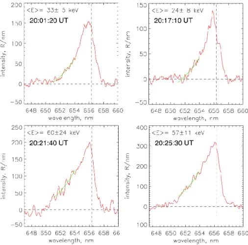
The experimental profiles, even after removal of the blended emissions, contains significant noise fluctuations. This is in addition to the error in the estimated energy. Fig-ure 9 presents several examples of the experimental profiles after removal of the blended emissions. The least-square fit-ted lines by Eq. (1) are marked with smooth curves.

The evolution of the estimated average energy during the event of interest is presented in Fig. 10. One can see that dur-ing the growth phase (20:00–20:20 UT) the energy of protons decreased gradually from ∼35 keV to ∼20 keV. The protons of the second population during the expansion phase (20:25– 20:28 UT) have the higher energy, ∼60 keV. We can note that during intervals of small Hα intensity (see Fig. 7b) the large discrepancy of estimated average energy mimics the rela-tively large noise fluctuation in the wavelength region used for the fitting procedure.

(10)

Fig. 9. Examples of observed Hα profiles (red lines) and the least-squares fit of the blue wing by Eq. (1) (green lines). <E> is an estimated average energy of precipitated protons. Dashed lines mark a position of non-shifted Hα line and zero intensity level.

Fig. 10. Evolution of the estimated average energy of precipitated protons.

Due to specific features of the excitation cross sections, the efficiency of the hydrogen excitation decreased with increas-ing of particle energy. Therefore, the estimated energy flux of proton precipitation does not directly correspond to the average proton energy or intensity of the hydrogen emission. During the growth phase, the estimated energy flux of proton precipitation then decreased from ∼6.5×10−4Joule/m2s to

∼2.5×10−4Joule/m2s. During the intensification of 20:25– 20:28 UT the proton energy flux was ∼2.2×10−3Joule/m2s.

6 Discussion

6.1 Modelling of the degradation of the proton-H atom flux

Some attempts to estimate the parameters of precipitating protons from the hydrogen emission profiles were under-taken already in early papers; see review in Eather (1967). Such estimates are usually based on a comparison of ob-served profiles with the ones obtained by some theoretical calculations modelling the degradation of the proton-H atom flux in the atmosphere. However, the solution to this prob-lem is complicated by several factors, which forced critical concerns in many previous papers. First, the cross sections

(11)

for collisional reactions of protons and H-atoms with atmo-spheric gases in the energy range needed for theoretical cal-culations were published only in Van Zyl et al. (1978, 1980). Many previous papers were based on erroneous assumptions about the energy dependencies of these cross sections; see review in McNeal and Birely, (1973).

Second, even after publication of these cross sections, many authors continued to discuss such a characteristic as a “Doppler shift of the profile maximum” (Takahashi and Fukunishi, 2001). However, the elementary consideration of the modern cross sections demonstrates that this shift is basically determined by the position of the maximum in the energy dependence of the effective cross section of hydro-gen emission (∼1 keV) and by the pitch-angle distribution in the precipitation flux at low energies (<10 keV). Higher-energetic particles with the large pitch angles can also give a contribution to the maximum of the hydrogen line profile, but this contribution is much weaker because of the decrease in excitation efficiency at the larger energies (>20 keV). Be-sides, in some papers, the dependence of the efficiency of hydrogen emission excitation on initial proton energy is ig-nored (for example, Mende et al. (2001)).

Third, the theoretical models of proton-H atom flux trans-port in the atmosphere have problems related to specific fea-tures of the various algorithms. The most powerful approach is the Monte-Carlo method, based on direct simulation of the particle trajectories in the framework of a “collision-by-collision” algorithm. This approach was used, for exam-ple, in the following papers (Davidson, 1965; Kozelov and Ivanov, 1992; Kozelov, 1993, 1994; Lorentzen et al., 1998; Synnes et al., 1998), where the authors obtained many trans-port characteristics of the proton-H atom fluxes in the Earth’s atmosphere. The Monte-Carlo algorithms naturally take into account the collisional scattering of particles and the influ-ence of the inhomogeneous magnetic field. The calculation precision is limited only by the errors in the collision cross sections. The statistical discrepancy can be obtained in the algorithm itself during the model calculation.

A simpler method of transport calculations is based on the continuous slowing down approximation (CSDA) (Edgar et al., 1973, 1975). In reality, after several collisions with atoms and molecules of an absorber, the precipitated proton flux comes to a charge equilibrium state defined by the rela-tion between cross secrela-tions of charge exchange and stripping processes. On average, the energy loss of a monodirectional proton-hydrogen atom flux in the charge equilibrium state is described by the equation dE/dx=−L(E), where L(E) is the loss function (Edgar et al., 1973). The more refined version of the CSDA for non-equilibrium proton-hydrogen atom flux was considered in Decker et al. (1996). How-ever, the methods based on CSDA cannot directly take into account such effects as the discrete nature of the energy loss, collisional angle scattering, and the influence of the magnetic field.

Several authors have developed different algorithms to solve directly the transport equation for particle fluxes (Jasperse and Basu, 1982; Basu et al., 1990; Galand et al.,

1997). Usually the algorithms need additional assumptions about transport processes to simplify the numerical calcula-tions. However, the common problem of such algorithms is the number of interpolation procedures needed to recalculate the distribution of particle fluxes after each step of the spa-tial variable. Therefore, the algorithms tend to accumulate a systematic error which is hardly detectable in the frame-work of the method itself. The checking methods (for exam-ple, checking of the energy conservation rule, increasing of cell number in the phase space, etc.) cannot solve the prob-lem. Usually the systematic error leads to artifacts near the boundaries of the spatial region occupied by the dissipated particles. In a paper by Decker et al. (1996) the above-mentioned three theoretical techniques were tested by pre-cisely the same incoming parameters and input conditions. For the simplest conditions (without collisional angle scat-tering and magnetic field, and with a simplified set of cross sections) it was shown that these theoretical techniques gave practically the same distribution of the particle fluxes in the dissipation region.

6.2 Lateral spreading and structure of hydrogen emission region

It is well-known that the hydrogen emission region is diffuse because the precipitated protons undergo charge-exchange collisions and thereby spend a part of the time as neutral hydrogen atoms that cross magnetic field lines. David-son (1965) modeled the lateral spread of hydrogen emission in the atmosphere due to this process using a thin sheet of ini-tial precipitated protons. The characteristic scale of the hy-drogen emission zone was found to be ∼100 km. Therefore, the spatial structure observed in our case for the second pop-ulation of protons seems very strange in that it is less diffuse, or more structured than one would expect. Kozelov (1993) provided a more detailed study of the lateral spreading effect in the dipolar magnetic field and showed that the spreading effect decreases with the increasing of the initial proton en-ergy. Thus, the observed structure is additional evidence of the higher energy of precipitated protons, relative to the pro-tons in the diffuse aurora.

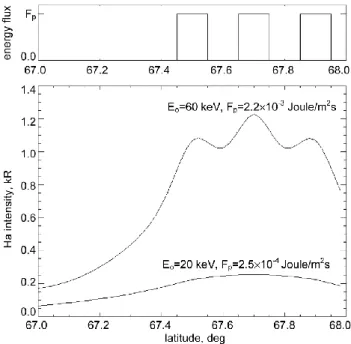
Let’s consider the ionospheric spatial structures produced by a set of three sheets of monoenergetic proton precipi-tation with a distance of ∼20 km between the centers of the sheets. The longitudinal orientation of the sheets is as-sumed, and the latitudinal section of simulated precipita-tion structure is shown in top panel of Fig. 11. A down-ward isotropic pitch-angle distribution in precipitation flux is assumed. The precipitation is characterized by values of initial energy (Eo) and of energy flux (Fp). The

simpli-fied model from Kozelov et al. (1995), based on the re-sults of detailed Monte-Carlo transport modeling, was used to calculate the Hα luminosity structure resulting from such precipitation for different values of Eo and Fp. The

bot-tom panel of Fig. 11 presents the simulation results for two cases: Eo=20 keV, Fp=2.5×10−4Joule/m2s and Eo=60 keV,

(12)

characteristics of a second population of the precipitated pro-tons observed at 20:25–20:28 UT.

The results illustrate that the structure of the precipita-tion for Eo=60 keV is easily observed in the spatial

lumi-nosity distribution, while no structure is seen for Eo=20 keV.

The variations of 10–20% in the simulation luminosity for

Eo=60 keV correspond well to the observed spatial

luminos-ity variations in 20:25–20:27 UT at 0◦–30◦zenith angles; see Fig. 5c. This structure is absent in Fig. 5d, therefore, we can deduce that this is the structure of hydrogen emission, but not of other emissions excited by electron precipitation. So, the simulation results of the spatial distribution of luminosity also supports the conclusion about the higher characteristic energy of protons precipitated in the second population. 6.3 Mechanisms of proton precipitation at different phases

of the substorm

Before the substorm onset, and during the late growth phase of the event considered here the morphology of the hydrogen emission is comparable to previous observations (Yevlashin and Yevlashina, 1980). The wide (>100 km) diffuse region of the equatorward hydrogen emission is slowly moving to-wards the equator. The integrated intensity of Hα emission was 300–500 R, the average energy of the precipitated pro-ton was 20–35 keV, and the estimated energy flux of propro-ton precipitation was ∼3×10−4Joule/m2s, which is typical for the region (Hardy et al., 1991). The proton drift in the large-scale electric and magnetic fields and subsequent interaction with ion-cyclotron waves lead to pitch-angle diffusion of the proton flux in the plasma sheet and, therefore, to the precip-itation in the atmosphere. Inside the region of the hydrogen emission there are more mobile electron structures. The most equatorial discrete electron arc had several intensifications and the last of them (∼20:16 UT) led to the auroral breakup (∼20:21 UT). In the breakup, or onset, the arc was located at the poleward boundary of the hydrogen emission region.

The main peculiarity of this event is a clear manifestation of the dynamical structure of the hydrogen emission evolu-tion during the substorm at the temporal scales of 2–3 min after onset, when both the intensity and the shape of the hy-drogen emission line profile varied dramatically. During the first 2 min after onset, the hydrogen line was also increas-ing in intensity. However, when the electron arc expanded poleward with the development of the westward traveling surge (WTS), the hydrogen emission was absent in the lead-ing edge of the WTS. The same features had been noted pre-viously by Takahashi and Fukunishi (2001) and Deehr and Lummerzheim (2001). The next intensification of the hydro-gen emission appeared 2–3 min later on the north side of the field of view inside the region of active aurora. Deehr and Lummerzheim (2001) found that “the H emission expands poleward after the formation of the N-S oriented arcs”. In our case, the N-S oriented electron arcs were also present during the Hα intensification from 20:24 to 20:28 UT; see Fig. 4, all-sky TV image for 20:26 UT. The Hα emission intensifi-cation region was located a bit northward from the poleward

Fig. 11. Hα luminosity as a function of latitude, stimulated by three regions of precipitated protons. Top panel is a latitudinal section of precipitation structure. Bottom panel presents the spatial struc-tures of the column-integrated luminosity for two cases of proton precipitation parameters.

boundary of the hydrogen emission at the end of the growth phase. However, as we deduce from the hydrogen line pro-file, the average energy of the precipitated protons during 20:24–20:28 UT was higher by a factor of 2–3 than before the breakup. An increase of the particle flux at energies up to

>300 keV was found by Sergeev and Kubyshkina (1996) 3– 4 min after a substorm onset in data from low-altitude satel-lites.

During the expansion phase of substorm, the earthward in-jection of energetic particles occurs under the influence of large, short-lived electric fields. In the course of this in-jection, the particles are subjected to both impulsive paral-lel and perpendicular acceleration and nonadiabatic motion. The convection surge mechanism (Mauk, 1986) for the ion acceleration is efficient in producing energetic particles, es-pecially when nonadiabatic effects are concerned (Delcourt et al, 1994). The dynamics of the non-adiabatic motion re-gion of protons during the development of the expansion phase in the equatorial plane of the nightside magnetosphere at 5–8 RE was analyzed in Kozelov and Kozelova (2003),

using data from the CRRES satellite and the adapted time-dependent magnetospheric model. The spatial scale of the transition region (boundary) from adiabatic to non-adiabatic ion motion was found to be about 1 RE. This boundary is

bent in a radial direction before the beginning of an expan-sion phase and then is moving in a tailward direction. This movement is accompanied by fast changes of pitch-angle dis-tribution in proton flux. Therefore, we can assume that the second population of protons in the event discussed is prob-ably produced by pitch-angle scattering of protons due to

(13)

the non-adiabatic motion in the region of local dipolarization near the equatorial plane.

Thus, the characteristics of the proton precipitation fluxes before the leading edge of WTS and inside the WTS re-gion appear to be different from one another. The possible physical mechanisms that lead to the precipitation differ, too. Therefore, we have strong evidence for the existence of two different populations of protons.

7 Conclusions

The paper describes the results of coordinated, optical ground-based observations of the auroral substorm on 26 March 2004 in the Kola Peninsula. In addition to the usual observatory equipment, consisting of an all-sky TV camera and a scanning photometer, a special imaging spectrograph with high spectral and temporal resolution was used. The data from this device allowed us to use the Doppler profile of the Hα hydrogen emission to estimate the variation in the en-ergy of the precipitating proton flux and the proton emission intensity.

Two different populations of precipitated proton flux were observed during the event. The first of them was a diffuse proton precipitation that is usually observed in the evening sector of the auroral oval and located equatorward of the dis-crete electron precipitation. The average energy of the pro-tons during this precipitation was ∼20–35 keV, the energy flux was ∼3×10−4Joule/m2s.

The second population of precipitated protons was sepa-rated from the first one by the breakup, or onset arc (bound-ary of WTS). The proton precipitation was observed 1–2 min after the breakup and 4–5 min into the expansion phase of the substorm into the zone of bright discrete auroral structures. The average energy of the protons during this precipitation was ∼60 keV, the energy flux was ∼2.2×10−3Joule/m2s. We believe that the most probable mechanism of precip-itation was pitch-angle scattering of protons due to non-adiabatic motion in the region of local dipolarization near the equatorial plane.

Acknowledgements. The work was partly supported by the basic research programs of Russian Academy of Sciences ”Solar activity and physical processes in the Sun-Earth system” and the Division of Physical Sciences of RAS ”Plasma processes in the solar system”. Authors thank the Polar Geophysical Institute for the data from the Lovozero observatory and all referees for helpful comments.

Topical Editor U.-P. Hoppe thanks C. Deehr and two other ref-erees for their help in evaluating this paper.

References

Akasofu, S.-I.: Polar and magnetospheric substorms. D. Reidel Publ., Dordrecht-Holland, 1968.

Basu, B., Jasperse, J. R., and Grossbard, N. J.: A numerical solution of the coupled proton-H atom transport equations for the proton aurora, J. Geophys. Res., 95, 19 069–19 078, 1990.

Chamberlain, J. W.: Physics of the aurora and airglow, Academic Press, San Diego, Calif. 1961.

Davidson, G. T.: Expected spatial distribution of low-energy pro-tons precipitated in the auroral zones, J. Geophys. Res., 70, 1061–1068, 1965.

Decker, D. T., Kozelov, B. V., Basu, B., Jasperse, J. R., and Ivanov, V. E.: Collisional degradation of the proton-H atom fluxes in the atmosphere: A comparison of theoretical techniques, J. Geophys. Res., 101, 26 947–26 960, 1996.

Deehr, C. and Lummezheim, D.: Ground-based optical observa-tions of hydrogen emission in the auroral substorm, J. Geophys. Res., 106, A1, 33–44, 2001.

Delcourt, D. C., Martin, R. F., Jr. and Alem, F.: A simple model of magnetic moment scattering in a field reversal, Geophys. Res. Lett., 21, 1543–1546, 1994.

Delcourt, D. C., Sauvaud, J.-A., Martin, R. F., Jr., and Moore, T. E.: On the nonadiabtic precipitation of ions from the near-Earth plasma sheet, J. Geophys. Res., 101, 8, 17 409–17 418, 1996. Eather, R. H.: Auroral proton precipitation and hydrogen emission,

Phys. Rev., 5, 207–285, 1967.

Edgar, B. C., Porter, H. S., and Green, A. E. S: Proton energy de-position in molecular and atomic oxygen and applications to the polar cap, Planet. Space Sci., 23, 787–804, 1975.

Edgar, B. C., Miles, W. T., and Green, A. E. S.: Energy deposition of proton in molecular nitrogen and applications to the proton auroral phenomena, J. Geophys. Res., 78, 6595–6606, 1973. Fleischmann, H. H., Barnett, C. F., and Ray, J. A.: Small-angle

scat-tering in stripping collisions of hydrogen atoms having energies of 1–10 keV in various gases, Phys. Rev. A, 10, 569–583, 1974. Fleischmann, H. H., Young, R. A., and McGowan, J. W.:

Differ-ential charge-transfer cross sections for collisions of H+ on O2,

Phys. Rev., 153, 19–22, 1967.

Fukunishi, H.: Dynamic relationship between proton and electron auroral substorms, J. Geophys. Res., 80, 553–574, 1975. Galand, M., Lilensten, J., Kofman, W., and Sidje, R. B.: Proton

transpoprt model in the ionosphere, 1, Multistream approach of the transport equations, J. Geophys. Res., 102, 22 261–22 272, 1997.

Galperin, Yu. I.: Hydrogen emission and two types of auroral spec-tra, Planet. Space Sci., 1, 1, 57–62, 1959.

Galperin, Y. I., Kovrazhkin, R. A., Ponomarev, Y. N., Crasnier, J., and Sauvaud, J. A.: Pitch angle distributions of auroral protons, Ann. Geophys., 32, 109–115, 1976.

Gao, R. S., Johnson, L. K., Hakes, C. L., Smith, K. A, and Stebbing, R. F.: Collisions of kiloelectronvolt H+ and He + with molecules at small angles: Absolute differential cross sections for charge transfer, Phys. Rev. A., 41, 5929–5933, 1990.

Gattinger, R. L. and Vallance Jones, A.: Quantitative spectroscopy of the aurora. II. The spectrum of medium intensity aurora be-tween 4500 and 8900 ˚A, Can. J. Phys., 52, 2343–2356, 1974. G´erard, J.-C., Hubert, B., Grard, A., Meurant, M., and Mende, S. B.:

Solar wind control of auroral substorm onset locations observed with the IMAGE-FUV imagers, J. Geophys. Res., 109(A03208), doi:10.1029/2003JA010129, 2004.

(14)

Hardy, D. A., McNeil, W. J., Gussenhoven, M. S., and Brautigam, D. H.: A statistical model of auroral ion precipitation. 2. Func-tional representation of the auroral pattern, J. Geophys. Res., 96, 5539–5547, 1991.

Hedin, A. E.: MSIS-86 thermospheric model, J. Geophys. Res., 92, 4649–4662, 1987.

Jasperse, J. R. and Basu, B.: Transport theoretic solutions for auro-ral proton and H atom fluxes and related quantities, J. Geophys. Res., 87, 811–822, 1982.

Kirillov, A. S.: Calculation of rate coefficients of electron energy transfer processes for molecular nitrogen and molecular oxygen, Adv. Space Res., 33, 998–1004, 2004.

Kozelov, B. V., Ivanov ,V. E., and Sergienko T. I.: Simplified al-gorithm for precise calculation of spatial distributions in com-bined electron-proton-hydrogen atom aurora, Geomagnetism and aeronomy (English translation), 34, 5, 644–646, 1995.

Kozelov, B. V. and Kozelova, T. V.: Dynamics of domains of nona-diabatic particle motion in the near magnetosphere during a sub-storm, Geomagnetism and aeronomy (English translation), 43, 4, 488–497, 2003.

Kozelov, B. V. and Ivanov, V. E.: Monte-Carlo calculation of proton-hydrogen atom transport in N2, Planet. Space Sci., 40,

1503–1511, 1992.

Kozelov, B. V.: Influence of the dipolar magnetic field on transport of proton-H atom fluxes in the atmosphere, Ann. Geophys., 11, 697–704, 1993.

Kozelov, B. V.: Calculation of Hβ emission in aurora. Comparison with observation, Geomagnetism and aeronomy, 34, 5, 86–90, 1994.

Kozelova, T. V., Kozelov, B. V., and Lazutin, L. L.: Local gradient of energetic ion flux during dipolarization on 6-7 RE, Adv. Space

Res., 33, 774–779, 2004.

Lanchester, B. S., Galand, M., Robertson, S. C., Rees, M. H., Lum-merzheim, D., Furniss, I., Peticolas, L. M., Frey, H. U., Baum-gardner, J., and Mendillo, M.: High resolution measurements and modeling of auroral hydrogen emission line profile, Ann. Geo-phys., 21, 1629–1643, 2003,

SRef-ID: 1432-0576/ag/2003-21-1629.

Lorentzen, D. A., Sigernes, F., and Deehr, C. S.: Modeling and observations of dayside auroral hydrogen emission Doppler pro-files, J. Geophys. Res., 103(A8), 17 479–17 488, 1998.

Mauk, B. H.: Quantitative modeling of the “convection surge” mechanism of ion acceleration, J. Geophys. Res., 91, 13 423– 13 431, 1986.

McNeal, R. J. and Birely, J. H.: Laboratory studies of collisions of energetic H+ and hydrogen with atmospheric constituents, Rev. Geophys. Space Phys., 11, 633–693, 1973.

Mende, S. B., Frey, H. U., Lampton, M., Gerard, J.-C., Hubert, B., Fuselier, S., Spann, J., Gladstone, R., and Burch, J. L.: Global observations of proton and electron auroras in a substorm, Geo-phys. Res. Lett., 28, 6, 1139–1142, 2001.

Montbriand, L. E.: The proton aurora and auroral substorm, In: “The Radiating Atmosphere, (Ed.) McCormac, B. M., D. Reidel Publishing CoDordrecht, 366–373, 1971.

Newman, J. H., Chen, Y. S., Smith, K. A., and Stebbing, R. F.: Differential cross sections for scattering of 0.5, 1.5 and 5.0 keV hydrogen atoms by He, N2and O2, J. Geophys. Res., 91, 8947–

8954, 1986.

Samson, J. C., Lyon, L. R., Newell, P. T., Creutzberg, F., and Xu, B.: Proton aurora and substorm intensification, Geophys. Res. Lett., 19, 2167–2170, 1992.

Sauvaud, J.-A. and Winckler, J. R.: Dynamics of plasma, energetic particles, and fields near synchronous orbit if the nighttime sec-tor during magnetospheric subssec-torm, J. Geophys. Res., 85(A5), 2043–2056, 1980.

Sergeev, V. A. and Kubyshkina, M. V.: Low altitude image of parti-cle acceleration and magnetospheric reconfiguration at substorm onset, J. Geomag. Geoelectr., 48, 877–885, 1996.

Sergienko, T. I. and Ivanov, V. E.: A new approach to calculate the excitation of atmospheric gases by auroral electron impact, Ann. Geophys., 11, 717–727, 1993.

Søraas, F., M˚aseide, K., Torheim, P., and Aarsnes, K.: Doppler-shifted auroral Hβ emission: a comparison between observations and calculations, Ann. Geophys., 12, 1052–1064, 1994, SRef-ID: 1432-0576/ag/1994-12-1052.

Søraas, F., Lindalen, H. R., M˚aseide, K., Egeland, A., Sten, T. A., and Evans, D. S.: Proton precipitation and the Hβ emission in a postbreakup auroral glow, J. Geophys. Res., 79, 1851–1859, 1974.

Synnes, S. A., Søraas, F., and Hansen, J. P.: Monte-Carlo simulation of proton aurora, J. Atmos. Sol-Terr. Phys., 60, 1695, 1998. Takahashi, Y., and Fukunishi, H.: The dynamics of the proton

au-rora in auau-roral breakup events, J. Geophys. Res., 106, A1, 45-63, 2001.

Van Zyl, B., Neumann, H., Le, T.Q., and Amme, R. C.: H+N2and

H+O₂collisions: Experimental charge-production cross sections and differential scattering calculations, Phys. Rev. A., 18, 506– 516, 1978.

Van Zyl, B. and Neumann, H.: Hα and Hβ emission cross sections for low-energy H and H+ collisions with N2and O2, J. Geophys.

Res., 85, 6006–6010, 1980.

Vegard, L.: Hydrogen showers in the auroral region, Nature, 144, 1089–1090, 1939.

Yevlashin, L. S. and Yevlashina, L. M.: Field align electric field as main source of particle acceleration during auroral substorm. In: “The Structure of auroral substorm (Results of IMS)”, Apatity, Kola Science Centre RAS, 45–53, 1980.

Yevlashin, L. S.: Hydrogen emission in auroras and the precipita-tion of auroral protons, In: “Physics of the near-earth Space”, part 3, Apatity, Kola Science Centre RAS, 500–548, 2000. Yevlashin, L. S.: Space-time variations of hydrogen in auroras and

their connection with magnetic disturbances, Geomagnetism and aeronomy, 1, 1, 54–58, 1961.