HAL Id: tel-01164995
https://tel.archives-ouvertes.fr/tel-01164995
Submitted on 18 Jun 2015HAL is a multi-disciplinary open access archive for the deposit and dissemination of sci-entific research documents, whether they are pub-lished or not. The documents may come from teaching and research institutions in France or abroad, or from public or private research centers.
L’archive ouverte pluridisciplinaire HAL, est destinée au dépôt et à la diffusion de documents scientifiques de niveau recherche, publiés ou non, émanant des établissements d’enseignement et de recherche français ou étrangers, des laboratoires publics ou privés.
dynamic games
Juan Pablo Maldonado Lopez
To cite this version:
Juan Pablo Maldonado Lopez. Some links between discrete and continuous aspects in dynamic games. General Mathematics [math.GM]. Université Pierre et Marie Curie - Paris VI, 2014. English. �NNT : 2014PA066271�. �tel-01164995�
École Doctorale de Sciences Mathématiques de Paris Centre
Thèse de doctorat
Discipline : Mathématiques Apliquées
présentée par
Juan Pablo MALDONADO LOPEZ
Some links between discrete and continuous
aspects in dynamic games
dirigée par Sylvain SORIN
Soutenue le 4 novembre 2014 devant le jury composé de :
M. Sylvain SORIN
Université Pierre et Marie Curie directeur
M. Rida LARAKI
Université Paris Dauphine
examinateur
M. Tristan TOMALA
HEC Paris
examinateur
M. Jean-Paul ALLOUCHE
Université Pierre et Marie Curie examinateur
M. Stéphane GAUBERT
INRIA-Saclay
examinateur
M. Nicolas VIEILLE
HEC Paris
rapporteur
M. Martino BARDI
Università degli Studi di Padova rapporteur
M. Pierre CARDALIAGUET Université Paris Dauphine
président
Institut de Mathématiques de Jussieu 175, rue du Chevaleret
75 013 Paris
École Doctorale de Sciences Mathéma-tiques de Paris Centre Case 188 4 place Jussieu
Résumé
Résumé
Cette thèse étudie les liens entre a) les jeux en temps discret et continu, et b) les jeux à très grand nombre de joueurs identiques et les jeux avec un continuum de joueurs. Une motivation pour ces sujets ainsi que les contributions principales de cette thèse sont présentées dans le Chapitre 1. Le reste de la thèse est organisé en trois parties. La Partie I étudie les jeux différentiels à somme nulle et à deux joueurs. Nous décrivons dans le Chapitre 3 trois approches qui ont été proposées dans la littérature pour établir l’existence de la valeur dans les jeux différentiels à deux joueurs et à somme nulle, en soulignant les liens qui existent entre elles. Nous fournissons dans le Chapitre 4 une démonstration de l’existence de la valeur à l’aide d’une description explicite des stratégies ‘-optimales. Le Chapitre 5 établit l’équivalence entre les solutions de minimax et les solutions de viscosité pour les équations de Hamilton-Jacobi-Isaacs. La Partie II porte sur les jeux à champ moyen en temps discret. L’espace d’action est supposé compact dans le Chapitre 6, et fini dans le Chapitre 7. Dans les deux cas, nous obtenons l’existence d’un ‘- équilibre de Nash pour un jeu stochastique avec un nombre fini de joueurs identiques, où le terme d’approximation tend vers zéro lorsque le nombre de joueurs augmente. Nous obtenons dans le Chapitre 7 des bornes d’erreur explicites, ainsi que l’existence d’un ‘-équilibre de Nash pour un jeu stochastique à durée d’étape évanescente et à un nombre fini de joueurs identiques. Dans ce cas, le terme d’approximation est fonction à la fois du nombre de joueurs et de la durée d’étape. Enfin, la Partie III porte sur les jeux stochastiques à durée d’étape évanescente, qui sont décrits dans le Chapitre 8. Il s’agit de jeux où un paramètre évolue selon une chaîne de Markov en temps continu, tandis que les joueurs choisissent leurs actions à des dates discrètes. La dynamique en temps continu dépend des actions des joueurs. Nous considérons trois évaluations différentes pour le paiement et deux structures d’information : dans un cas, les joueurs observent les actions passées et le paramètre, et dans l’autre, seules les actions passées sont observées.
Mots-clefs
Jeux dynamiques à somme nulle, jeux différentiels à somme nulle, jeux à champ moyen en temps discret, jeux stochastiques à étape evanescente
Some links between discrete and continuous in dynamic
games
Abstract
In this thesis we describe some links between a) discrete and continuous time games and b) games with finitely many players and games with a continuum of players. A motivation to the subject and the main contributions are outlined in Chapter 2. The rest of the thesis is organized in three parts: Part I is devoted to differential games, describing the different approaches for establishing the existence of the value of two player, zero sum differential games in Chapter 3 and pointing out connections between them. In Chapter 4 we provide a proof of the existence of the value using an explicit description of ‘-optimal strategies and a proof of the equivalence of minimax solutions and viscosity solutions for Hamilton-Jacobi-Isaacs equations in Chapter 5. Part II concerns discrete time mean field games. We study two models with different assumptions, in particular, in Chapter 6 we consider a compact action space while in Chapter 7 the action space is finite. In both cases we derive the existence of an ‘-Nash equilibrium for a stochastic game with finitely many identical players, where the approximation error vanishes as the number of players increases. We obtain explicit error bounds in Chapter 7 where we also obtain the existence of an ‘-Nash equilibrium for a stochastic game with short stage duration and finitely many identical players, with the approximation error depending both on the number of players and the duration of the stage. Part III is concerned with two player, zero sum stochastic games with short stage duration, described in Chapter 8. These are games where a parameter evolves following a continuous time Markov chain, while the players choose their actions at the nodes of a given partition of the positive real axis. The continuous time dynamics of the parameter depends on the actions of the players. We consider three different evaluations for the payoff and two different information structures: when players observe the past actions and the parameter and when players observe past actions but not the parameter.
Keywords
Zero sum dynamic games, zero sum differential games, discrete time mean field games, short stage stochastic games.
Contents
1 Introduction 1
1.1 Thématiques abordées dans cette thèse . . . 1
1.2 Jeux différentiels . . . 1
1.3 Jeux à champ moyen en temps discret . . . 4
1.4 Jeux stochastiques à étape courte . . . 5
1.5 Nos contributions principales . . . 7
2 Introduction 9 2.1 Motivation and examples . . . 9
2.2 Contents of this thesis . . . 10
2.3 Differential games . . . 12
2.4 Discrete time mean field games . . . 20
2.5 Zero-sum stochastic games with short-stage duration . . . 23
2.6 Short stage stochastic games . . . 25
2.7 Main contributions . . . 29
I Differential games
31
3 Value of zero-sum differential games 33 3.1 Introduction . . . 333.2 The discrete game approach . . . 38
3.3 The viscosity approach . . . 42
3.4 The strategic approach . . . 45
3.5 Some links between these approaches . . . 47
4 A strategy-based proof of the existence of the value in zero-sum differ-ential games 51 4.1 Comparison of trajectories . . . 51
4.2 Differential Games . . . 55
4.3 Appendix . . . 59
5 Generalized solutions of HJI equations 61 5.1 The HJI equations . . . 61
5.2 Viscosity solutions . . . 63
5.3 Proximal solutions . . . 64
5.4 Minimax solutions . . . 65
II Discrete time mean field games
71
6 Discrete time mean field games 73
6.1 Introduction . . . 73
6.2 The mean field game equilibrium . . . 74
6.3 The game with a continuum of players . . . 76
6.4 The game with finitely many players . . . 77
7 Discrete time mean field games: The short-stage limit 83 7.1 Introduction . . . 83
7.2 The discrete time model . . . 84
7.3 A mean field game with frequent actions . . . 90
7.4 Concluding remarks . . . 93
III Stochastic games with frequent actions
97
8 Stochastic zero-sum games with a continuous time dynamics 99 8.1 Description of the general model . . . 998.2 Evaluation of the payoff . . . 101
8.3 No information on the state . . . 104
8.4 Standard signalling . . . 110
8.5 Some concluding remarks . . . 115
Chapitre 1
Introduction
1.1 Thématiques abordées dans cette thèse
Cette thèse porte principalement sur les jeux répétés (Partie I et III) à somme nulle et à deux joueurs. Dans ces jeux, les intérêts des joueurs sont opposés : le gain d’un joueur est la perte de l’autre.
Même dans ce cadre particulier, la théorie est assez riche et on voit intervenir des outils mathématiques très variés.
Une autre thématique qui nous intéresse, dans la Partie II, correspond aux jeux avec un très grand nombre des joueurs identiques, au sens où ils ont les mêmes fonctions de paiement et la même dynamique. Intuitivement, plus il y a de joueurs, plus l’analyse du jeu devient compliquée. Néanmoins, si les joueurs sont identiques, on peut controller cette complexité dans un terme dit de champ moyen qui sera défini plus tard.
Nous introduisons maintenant de façon plus précise les thématiques étudiés et les principales contributions.
1.2 Jeux différentiels
Soit (t1, x1) œ [0, 1] ◊ Rn. Soient U et V deux sous-ensembles compacts d’un espace
euclidien. On définit
U(t1) = {u : [t1,1] æ U, mesurable}, V(t1) = {v : [t1,1] æ V, mesurable}.
Si t1 = 0, ces ensembles seront notés U et V, respectivement.
Les ensembles U(t1), V(t1) sont les ensembles des fonctions de contrôle. Les éléments
de U, V sont dits contrôles ou actions.
Soit f : Rn◊U ◊V æ Rn et (u, v) œ U(t1)◊V(t1) une couple de fonctions de contrôle.
On considère l’équation différentielle ordinaire (EDO) suivante
x(t1) = x1, ˙x(t) = f(x(t), u(t), v(t)) p.s. sur [t1,1]. (1.1)
On fait l’hypothèse suivante sur f, pour que la trajectoire de l’EDO soit bien définie : Assumption 1.2.1. On suppose que la fonction f est continue, bornée, et qu’il existe
c >0 tel que pour tout (u, v) œ U ◊ V et x, y œ Rn :
Îf(x, u, v) ≠ f(y, u, v)Î Æ cÎx ≠ yÎ.
Avec cette hypothèse, on utilise le théorème de Carathéodory, [31, Chapter 2] pour déduire que l’EDO (1.1) possède une unique solution. L’évaluation de cette solution au temps s est noté par x[t1, x1,u, v](s) et est interprétée au sens étendu suivant : pour tout tœ [t1,1],
x[t1, x1,u, v](t) := x1+
⁄ t t1
f(x[t1, x1,u, v](s), u(s), v(s))ds.
Cela définit la dynamique. On pourrait aussi considérer l’intervalle [0, +Œ) pour définir la dynamique.
Pour bien spécifier un jeu différentiel, il faut en définir les objectifs et l’information et les stratégies de chaque joueur. Intuitivement, le joueur 1 choisit u et le joueur 2 v pour atteindre un objectif quantitatif ou un objectif qualitatif, qui nous allons spécifier tout de suite. Cette distinction entre objectifs quantitatifs et qualitatifs a déjà été faite par Isaacs [58], qui introduit les termes games of kind pour les jeux où l’objectif est qualitatif, et games of degree pour ceux où l’objectif est quantitatif.
On suppose que l’information est complète, ce qui veut dire que les joueurs connaissent touts les paramètres du jeu : état initial, dynamique, paiement et sa description.
Cas qualitatif
Pour le cas qualitatif, on considère le jeu de cible : l’objectif du joueur 1 est de faire que la variable d’état atteigne l’ensemble fermé M, dit cible, à la date t = 1, et l’objectif du joueur 2 est de l’en empêcher. On note ce jeu M(t1, x1).
On se pose les questions suivantes :
Question 1. 1. Pour une condition initiale (s, y) œ [t1,1] ◊ Rn donnée, peut-on
décider quel joueur a une stratégie gagnante ? 2. Construire des stratégies spécifiques.
On reformule la première question de la manière suivante :
Problem 1. Construire une partition de [t1,1] ◊ Rn en deux ensembles K1, K2,
satisfai-sant :
i) Si (1, x) œ K1, alors x œ M.
ii) Pour tout (s, y) œ K1, il existe une stratégie du joueur 1 telle que la trajectoire
induite reste sur K1.
iii) Pour tout (s, y) œ K2 il existe une stratégie du joueur 2 telle que la trajectoire
induite n’atteigne pas l’ensemble cible M à la date t = 1.
Un théorème qui permet établir une telle caractérisation est un théorème d’alter-native.
Nous n’étudions pas les jeux qualitatifs en détail, mais nous voudrions faire quelques remarques. Une complication importante dans les jeux en temps continu est qu’il n’existe pas une structure canonique d’information. Nos décrivons quelques exemples de structures d’information étudiées dans la littérature.
Un des premiers théorèmes d’alternative a été démontré par B.N. Pöeni nyj [79], qui a étudié le jeu de cible avec la classe de stratégies suivantes :
Definition 1.2.2. (‘-stratégies) On dit que les joueurs utilisent des ‘-stratégies dans le jeu de cible si le jeu est joué de la façon suivante :
i) Les deux joueurs connaissent (t1, x1).
ii) Le joueur 2 choisit ‘1 > 0 et une fonction de contrôle v1 qui sera joué dans
1.2. Jeux différentiels 3 iii) A partir de cette information, le joueur 1 choisit sa fonction de contrôle. iv) Au temps t1+ ‘1, le nouvel état est annoncé. La situation est répétée : le joueur
2 choisit ‘2, etc.
Avec cette structure d’information, plusieurs théorèmes d’alternative sont démontrés dans [79], sur des hypothèses différentes pour la dynamique et l’ensemble cible. Cependant, aucun lien avec le cas quantitatif n’est établi.
Krasovskii et Subbotin ont introduit la méthode d’extremal aiming [61] pour les jeux de cible. Cette méthode motive les résultats du Chapitre 4. Ils utilisent la notion de stratégies positionnelles, qui sont des limites de fonctions constantes par morceaux. En général, les fonctions de contrôle ainsi obtenues ne sont pas suffisamment régulières pour avoir une trajectoire bien définie, même au sens de Carathéodory. Donc, comme dans l’approache de Pöeni nyj, l’extremal aiming nous donne de l’information sur un jeu approximé.
Un théorème d’alternative plus récent a été proposé par Cardaliaguet [21] qui considère les stratégies non anticipatives, qui seront introduites dans le Chapitre 3. Ce résultat est important car il nous permet de résoudre le jeu de façon exacte.
Cas quantitatif
Soient ¸ : Rn ◊ U ◊ V æ [0, 1] et g : Rn æ [0, 1] deux fonctions qui représentent
respectivement un paiement courant et un paiement terminal. Pour le cas quantitatif, on peut considérer les évaluations de paiement suivantes :
1. Le jeu escompté à l’horizon infini : pour une histoire (x, u, v), le paiement que le joueur 1 reçoit du joueur 2 est :
⁄ Œ
t1
e≠fls¸(x[t1, x1,u, v](s), u(s), v(s))ds
avec fl > 0.
2. Le jeu à horizon fini : à la date t = 1, le joueur 2 paie au joueur 1 :
⁄ 1
t1
¸(x[t1, x1,u, v](s), u(s), v(s)ds + g(x[t1, x1,u, v](1)).
Ces jeux sont respectivement notés fl(t1, x1) et (t1, x1).
Pour résoudre un jeu quantitatif, il faut répondre aux questions suivantes :
Question 2. 1. Spécifier les conditions sur lesquelles on a existence et unicité de la fonction valeur et sa caractérisation.
2. Donner des stratégies ‘-optimales.
Comme dans le jeu de cible, on doit d’abord spécifier une structure d’information. Plusieurs structures d’information ont été proposées dans la littérature, voir Bardi et Capuzzo-Dolcetta [9, Chapter VIII].
Pour le jeu à l’horizon fini avec paiement courant ¸ © 0, on peut déduire de façon heuristique [58, Section 4.2] que le maxmin et le minmax sont des solutions des EDP suivantes
ˆw≠
ˆt (t, x) + supuœUvinfœV
+
f(x, u, v), Òxw≠(t, x), = 0 (1.2a)
ˆw+
ˆt (t, x) + infvœVusupœU
e
f(x, u, v), Òxw+(t, x)
f
avec les conditions au bord w≠(1, x) = w+(1, x) = g(x).
Cette déduction heuristique a été menée par Isaacs [58, Section 4.2]. Le lien entre EDP et jeux différentiels a été explicité dans le cadre des solutions de viscosité [33] par Evans et Souganidis [36]. La notion de solution de viscosité a été introduite par Crandall et Lions [33], voir aussi le livre de Lions [67].
Si, de plus, la condition d’Isaacs est satisfaite, i.e. si on a l’égalité suivante, sup
uœUvinfœV Èf(x, u, v), pÍ = infvœV supuœUÈf(x, u, v), pÍ
pour tous x, p œ Rn,on n’a qu’une seule équation, dite l’équation
d’Hamilton-Jacobi-Isaacs.
En utilisant la méthode d’extremal aiming pour un certain jeu de cible, Krasovskii et Subbotin montrent l’existence et l’unicité de la valeur pour le jeu à horizon fini. Dans leur preuve on obtient une description explicite des stratégies ‘-optimales. Le Chapitre 4 est inspiré de cette construction. Plus tard, Subbotin [97] propose une notion de solutions généralisées, les solutions de minimax qui permettent caractériser la valeur comme l’unique solution minimax de l’équation HJI. On montre l’équivalence des solutions de minimax avec les solutions de viscosité dans le Chapitre 5.
1.3 Jeux à champ moyen en temps discret
Les jeux à champ moyen en temps continu ont été introduits indépendamment par Huang, Caines et Malhamé [56, 57] et Lasry and Lions [64, 65, 66]. Le but de cette théorie est la modélisation de situations stratégiques avec un grand nombre des joueurs identiques et petits, au sens que l’influence d’un seul joueur sur les autres est négligeable.
Les jeux avec un continuum des joueurs ont déjà été étudies dans plusieurs contextes, notamment en économie, par Aumann [6], dans les jeux de congestion par Wardrop [106], et dans les jeux de population par Maynard Smith [73] et Maynard Smith et Price [74]. Ce qui est différent dans les jeux à champ moyen est l’aspect dynamique.
Les jeux à champ moyen ont une structure dite de backward-forward, qui est de façon intuitive l’idée suivante : chaque joueur "anticipe" un certain comportement moyen des autres dans un intervalle de temps et calcule son propre comportement optimal en prenant le comportement des autres comme un paramètre fixe. Donc, chaque joueur fait face à un problème de contrôle optimal. Si le comportement moyen des joueurs qui est induit par cette optimisation est le même que celui qui a été prédit, alors on dit que les joueurs sont dans un équilibre de champ moyen. On introduira des définitions précises dans le Chapitre 6.
Prenons l’exemple suivant, qu’on peut trouver dans les notes de Cardaliaguet [20] sur le cours de Lions au Collège de France.
Example 1.3.1. On considère N joueurs dans Rd. La position du joueur i a la date t est
donnée par
dXti= –itdt+
Ô 2dBi
t
Chaque joueur i minimise son coût :
⁄ T t 1 2|–is|2+ F (m≠is,N)ds + g(xiT, m≠iT,N) où m≠i s,N := N1≠1 q j”=i”xjs.
1.4. Jeux stochastiques à étape courte 5
De façon heuristique, si on prend la limite quand N æ +Œ, on obtient le système d’EDP suivant : ≠ˆu ˆt ≠ u + 1 2|Dxu|2 = F (x, m) in Rd◊ (0, T ); ˆm ˆt ≠ m + div(mDu) = 0 in R d ◊ (0, T ); m(0) = m0; u(x, T ) = g(x, m(T )) in Rd.
Ici, dans la première équation, u dénote la valeur du problème de contrôle optimal pour un joueur quelconque si la distribution des joueurs est donnée par m. La deuxième est une équation de Kolmogorov qui décrit l’évolution de la distribution des joueurs dans Rd.
Une motivation importante pour l’étude des jeux à champ moyen dans les applica-tions est l’obtention des ‘-équilibres de Nash dans les jeux à N joueurs, avec un terme d’approximation qui tend vers zero quand N tend vers l’infini.
Les jeux à champ moyen ont trouvé des applications, notamment dans certains pro-blèmes en économie, voir Guéant, Lasry et Lions [49]. On fait aussi référence au survey de Gomes et Saude [47] pour une collection de résultats récents et au livre de Bensoussan, Frehse et Yam [12] pour les liens avec la théorie du contrôle optimal de champ moyen.
La plupart de la littérature étudie les jeux à champ moyen en temps continu. Une exception importante est l’article de Gomes, Mohr et Souza [48], qui étude le comportement asymptotique d’un jeu à l’horizon fini quand l’horizon tend vers l’infini d’un jeu avec un continuum de joueurs en temps discret.
Par contre, nous considérons un horizon fini fixe et nous proposons une construction d’un équilibre de Nash approximé pour un jeu à N joueurs. Le modèle que l’on étude dans le Chapitre 6 est l’analogue en temps fini du jeu étudié par Adlakha, Johari et Weintraub [2].
Nous nous intéressons aussi aux situations où les joueurs interagissent "fréquemment". Pour donner un sens mathématique à cette expression, il faut introduire un temps exogène, disons R+. Ici, chaque joueur observe et contrôle une chaîne de Markov en temps continu
dont le générateur infinitésimal dépend du comportement moyen des autres. Les joueurs choisissent leurs actions aux instants de temps discrets, données par une partition de R+.
Nous décrivons ces modèles dans le cas à deux joueurs et somme nulle dans la Section suivante. L’analogue pour les jeux à champ moyen est introduit dans le Chapitre 7.
1.4 Jeux stochastiques à étape courte
Dans les jeux stochastiques en temps discret, il n’existe pas de notion de "durée" des étapes du jeu. Pour en introduire une, on considère un temps exogène, qui sera représenté par les nombres réels positifs, R+.
Cela nous permet de donner une définition de "durée" de la façon suivante : Soit = {t1, t2, . . .} une partition de R+. Le nombre réel fik := tk+1≠ tk est la durée de la
k-ème étape, qui commence à la date tk.
1.4.1 Dynamique
Soit un ensemble fini, dit espace de paramètres et on note par A et B les en-sembles d’action du joueur 1 et 2, respectivement. Soit “ : ◊ A ◊ B une fonction de paiement
Le paramètre évolue en temps continu, en suivant une chaîne de Markov homogène avec fonction de transition q : ◊ ◊ A ◊ B æ R, c’est a dire un fonction q qui satisfait, pour tout (Ê, a, b) œ ◊ A ◊ B :
0 Æ q(Ê, ÊÕ, a, b) < +Œ, ÊÕ”= Ê, et ÿ
ÊÕœ
q(Ê, ÊÕ, a, b) = 0.
Pour (a, b) œ A ◊ B fixé, la fonction de transition correspond à la vitesse avec laquelle le paramètre saute de Ê a ÊÕ. On note par P (·, Ê, a, b) le semi-groupe de transition
correspondant, c’est a dire une famille de fonctions P‘(·, a, b) : ◊ æ [0, 1] tels que
P(Êt+‘= ÊÕ|Êt = Ê, a, b) = P‘(Ê, ÊÕ, a, b) + o(‘),
pour tous t, ‘ Ø 0 et Ê, ÊÕ œ . L’application t ‘æ Pt(·, a, b) est solution de l’équation de
Chapman-Kolmogorov
˙Pt= Qa,bPt, P0= I,
où Qa,b:= (q(Ê, ÊÕ, a, b))
Ê,ÊÕ est le générateur de la chaîne de Markov avec semi groupe
de transition P (·, a, b).
1.4.2 Information et stratégies
Le jeu se déroule de la façon suivante : à la date tk, la valeur du paramètre est Êk,
que l’on suppose connu pour l’instant. Les joueurs choisissent leurs actions ak, bk. Puis, le
paramètre suit la chaîne de Markov avec générateur Qak,bk pour une période de temps fik.
Le nouveau paramètre Êk+1est observé à la date tk+1. Sa loi est Pfik(Êk,·, ak, bk).
Les actions restent constantes sur l’intervalle [tk, tk+1). Un paiement instantané
“s := “(Ês, ak, bk) est payé pour le jour 2 au joueur 1 à la date s œ [tk, tk+1). A la date
tk+1, le paiement d’étape “fik:=
stk+1
tk Ÿ(s)“sdsa été reçu pour le joueur 1 et la situation
se répète.
1.4.3 Evaluation du paiement
On considère les évaluations suivantes : Modèle A : Le jeu à horizon infini
On considère d’abord le cas où la durée et le poids de l’étape sont égaux.
Soit une probabilité décroissante sur N avec = (◊1, ◊2, . . .) et ◊1 < 1/ÎqÎ, où
ÎqÎ := max(Ê,a,b)œ ◊A◊B|q(Ê, Ê, a, b)|.
La k≠ième étape commence à la date sk := q¸<k◊¸. La dynamique du jeu est celle
décrite dans la Section 1.4.2, avec fik = ◊k.
Le paiement correspondant à l’histoire h := {Ê1, a1, b1, Ê2, a2, b2, . . .} est
Œ
ÿ
k=1
◊k“◊k,
1.5. Nos contributions principales 7 Modèle B : Le jeu stationnaire à étape courte
De façon intuitive, cet jeu est la discrétisation d’un jeu avec paiement
⁄ +Œ
0 fle
≠fls“sds,
avec fl > 0. Soit ” = {0, ”, 2”, . . .} une partition uniforme de R+, avec 0 < ” < 1/ÎqÎ.
Soit t”
j := (j ≠ 1)” la date de la j≠ième étape. Le jeu se déroule comme dans la Section
1.4.2.Le paramètre ” est ici la durée de l’étape.
Le paiement associé à l’histoire h := {Ê1, a1, b1, Ê2, a2, b2, . . .} est :
Jfl,”(h) := +Œÿ k=1 “fl,j,”, avec “fl,j,” := ⁄ t” j+1 t” j fle≠fls“sds.
On s’intéresse ici au comportement limite lorsque ” et fl tend vers zero. Modèle C : Le jeu a étape courte et évaluation générale
On peut aussi considérer le paiement
⁄ +Œ
0 Ÿ(s)“sds,
où Ÿ : R+æ R+ est une densité sur R+. Dans le cas particulier Ÿ(s) := fle≠fls avec fl > 0,
on retombe sur le jeu précédent.
Soit Ÿj,”:= Ÿ(t”j). Le paiement correspondant à l’histoire h := {Ê1, a1, b1, Ê2, a2, b2, . . .}
est JŸ,”(h) := +Œÿ j=1 “Ÿ,j,”, avec “Ÿ,j,” := ⁄ t” j+1 t” j Ÿ(s)“sds.
On suppose que les joueurs ont une mémoire parfaite.
Ces jeux ont une valeur par des arguments classiques. On s’intéresse au comporte-ment asymptotique de la fonction valeur quand la durée de l’étape tend vers zéro et à sa caractérisation.
1.5 Nos contributions principales
Le Chapitre 3 est un survey qui décrit dans un cadre unifié trois approches différentes pour établir l’existence de la valeur d’un jeu différentiel à deux joueurs et à somme nulle : i) L’ approche par discrétisation : Cet approche a été étudiée par Fleming [38] et Friedman [41, 42]. On s’intéresse ici aux propriétés de la fonction valeur des jeux en temps discret qui approximent le jeu différentiel en temps continu.
ii) L’approche EDP-solutions de viscosité. Cet approche revient à Isaacs [58, p.67], qui déduit une équation aux dérivées partielles pour la valeur, dite équation d’Hamilton-Jacobi-Isaacs. Evans and Souganidis [36] ont formalisé cette idée dans le cadre des solutions de viscosité.
iii) L’ approche stratégique de Krasovskii et Subbotin. On obtient ici l’existence de la valeur en utilisant des stratégies ‘-optimales explicites.
Nous établions des liens entre ces approches.
Dans le Chapitre 4, on propose un preuve courte de l’existence de la valeur pour les jeux différentiels à somme nulle, horizon fini et paiement terminal, basé sur la construc-tion de stratégies ‘-optimales. Notre preuve est inspiré par Krasovskii et Subbotin [61]. Cet Chapitre est issu d’un travail en commun avec Miquel Oliu-Barton et accepté pour publication dans Morfismos.
Pour conclure la première partie, dans le Chapitre 5 on montre l’équivalence entre la définition des solutions de viscosité, introduites par Crandall et Lions [33] et la no-tion de soluno-tions de minimax, introduites par Subbotin [96]. Notre preuve suit l’approche épigraphique de Frankowska [40]. A notre connaissance, l’équivalence entre solutions de viscosité et la définition "stratégique" des solutions de minimax n’a pas été explicité dans la littérature. Des idées similaires, mais dans un cadre plus général, avec un Hamiltonien mesurable en temps, ont été utilisés par Cardaliaguet et Plaskacz.
On introduit dans le Chapitre 6 un modèle pour les jeux à champ moyen en temps discret, inspiré par celui d’Adlakha, Johari et Weintraub [2]. Ce document fait partie d’un travail en cours avec S.C.P. Yam. On construit un ‘-équilibre de Nash pour le jeu à N joueurs, où le terme d’erreur ‘ tend vers zéro lorsque N tend vers l’infini. On n’obtient pas ici de borne explicite en termes de N.
On developpe les résultats précédents dans le Chapitre 7. On propose ici une preuve alternative qui nous permet d’obtenir une borne explicite. On introduit aussi la notion de durée d’une étape dans cet Chapitre, ce qui nous permet d’obtenir un objet limite qui sert à construire un équilibre de Nash approximé pour le jeu à un nombre fini des joueurs, ou le terme d’erreur dépend du nombre de joueurs et de la durée de l’étape. Ce travail a été soumis pour publication.
Pour conclure, dans le Chapitre 8, on étudie les jeux stochastiques à durée d’étape evanescente (deux joueurs, somme nulle) dans plusieurs structures d’information :
i) Les deux joueurs observent les actions mais pas le paramètre : dans ce cas le jeu se réduit a un jeu différentiel. Sous certains hypothèses de régularité, on construit des stratégies ‘-optimales, où ‘ dépend de la durée de l’étape.
ii) Signalisation standard : les joueurs observent le paramètre. De façon similaire au cas précédent, on obtient ici des objets limits pour construire stratégies ‘-optimales, ce qui permet de démontrer la convergence de la suite des fonctions valeur.
Chapter 2
Introduction
2.1 Motivation and examples
The aim of game theory is to model the strategic interactions between self-interested agents, which are called players but that might be companies, populations, humans, computers, animals or simply mathematical objects. Such interaction is called a game. When the game is simple enough, it can be represented in matrix form as in the example below.
Example 2.1.1. Let us consider the following game:
L R T 1 0 B 0 1
Player 1 is the row player, whose actions are Top or Bottom. Player 2, the column player, chooses among the actions Left or Right. A pure strategy for the players is a function from their past information, i.e. their private history, to their action sets. In this particular situation, the game is played only once, so the set of histories is empty and a pure strategy is simply an indication of which action to play. The pure strategy sets for player 1 and player 2 are respectively S1 and S2. In this example, S1 := {T, B} where T
denotes the strategy "play Top", and B the strategy "play Bottom". Similarly, S2:= {L, R}
where L and R are the strategies "play Left" and "play Right".
The numbers indicated on the matrix are the payoffs that player 1 receives from player 2. The situation pictured here is zero-sum because one player’s profit is at the others’ expense. It is one-shot because players will meet only once to play this game. If strategies ‡œ S1, · œ S2 are chosen, we denote the payoff by “(‡, ·).
Player 1 can choose his strategy optimally to ensure a payoff of at least w:= max
‡œS1·minœS2“(‡, ·) = 0.
In a similar way, player 2 can ensure that his payoff to player 1 is of at most w:= min
When a game is described as above, with all the strategies available to the players and the corresponding payoffs, we say the game is in normal form. The quantities w and w introduced in the example above are the maxmin and minmax in pure strategies.
In the way we have specified the game in this example, there is really nothing to study. The outcome depends on who "goes first": if player 2 chooses his strategy after player 1, he can play a best reply and ensure a payoff of 0. The way out of this situation is to allow the players to choose their actions randomly. This enlargement of the strategy space is crucial for it allows players to "hide" their actions: if player 2 is not sure about what player 1 will do, he can not enforce a bad payoff for him. Denote by , T the sets of mixed strategies of player 1 and 2. In this example, := ({T, B}) and T := ({L, R}) , where, for a finite set S, (S) denotes the set of probability distributions over S.
When mixed strategies are used, the following theorem holds:
Theorem 2.1.2. (Minmax Theorem, von Neumann, 1928 [103]) For every two-player,
zero-sum game with payoff function “ and finite action sets A, B there exist mixed strategies ‡úœ := (A) and ·úœ T := (B) for players 1 and 2, respectively, and a quantity v,
called value such that, for all (‡, ·) œ ◊ T :
“(‡ú, ·) Ø v, and “(‡, ·ú) Æ v.
This theorem is the cornerstone of game theory. A remark attributed to von Neumann is the following:
"As far as I can see, there could be no theory of games...without that theorem...I thought there was nothing worth publishing until the Minmax Theorem was proved."[28]
In the previous example, it is easy to see that the optimal strategies for each player are "play each action with probability 1/2" and the value is 1/2.
Of course, game theory has evolved far beyond the minmax theorem and constitutes an active area of research, comprising a large body of literature.
One important and particularly active area of research is repeated games. A repeated game is a game that is played more than once. This interaction may happen in discrete time or in continuous time. The repetition of a zero-sum game as the one above has no particular interest: playing i.i.d an optimal strategies each stage is optimal, and any normalized evaluation gives the value of the one-shot game. The interesting object to study are games where "something" changes with time. What exactly "something" means depends specifically on the model. The richness of the theory of repeated games comes from the fact that seemingly related models require very different tools, coming from many different branches of mathematics. Reciprocally, seemingly unrelated models can be studied with similar tools.
2.2 Contents of this thesis
This thesis concerns mostly two player, zero-sum repeated games (Part I and III). These are games where the players have opposite interests: one player’s gain is at the other player’s expense. Thus, players are in open competition.
Restricting to two player, zero-sum games is, admittedly, a simplification, but this by no means implies that the theory is trivial. We hope to convince the reader that the zero-sum case is already rich enough, covering different mathematical tools and ideas and leaving interesting questions unanswered.
2.2. Contents of this thesis 11 Let us provide some motivating examples. This discussion is completely informal, proper definitions are introduced later.
Example 2.2.1. (A game with two states)
L R
T a+,p11 a12
B a21 a22
Here, a+,p11 means that if (T, L) is played, player 1 receives a payoff of a11 and the game
moves to the state + with probability p. The payoff matrix of state + is
L R T b11 b12 B b≠,q 21 b22 . Here b≠,q
21 means that if (B, L) is played, then player 1’s payoff is b21 and the game returns
with probability q to the state ≠, whose payoff matrix is the one above. Let us assume that the game is played infinitely often and denote by “k the stage payoff, that is, the payoff
player 1 receives the k≠th time the game is played, for k = 1, 2, . . . . Let ⁄ œ (0, 1]. The total payoff for player 1 is then:
Œ
ÿ
k=1
⁄(1 ≠ ⁄)k≠1“k.
Here, the value of the game depends on whether the initial state is + or ≠.
In the example above, the factor (1≠⁄) serves to represent the fact that the players are impatient and prefer current payoffs rather than future. An alternative interpretation, as provided in Shapley’s [87] original paper is that of stopping probability: ⁄ is the probability that the game stops, so that ⁄(1 ≠ ⁄)k is the probability that the game stops after k + 1
stages.
The game above is played in discrete time. However, for many applications it is inter-esting to consider also games in continuous time, as motivated by the following example. Example 2.2.2. (Lion and Man) A lion and a man in a closed arena have equal maximum
speed. What should the lion do to ensure his lunch?
This example has been attributed to Rado by Littlewood [70, p.135] and remained a mathematical challenge for some time. It turns out that the lion can get as close as it wants to the man, but the man can avoid capture. We will not describe this here, but refer to Littlewood [70, p.135] for the original proof, attributed to Besicovitch.
The main difficulty in continuous time is that there is no canonical information pattern. This in turn implies that there is no canonical definition of strategies. Thus, the outcome of the game may depend on the information pattern adopted. This complication does not arise in discrete time, as we can unambiguously define the information available to the players at the beginning of each stage.
Several information patterns have been adopted in the differential games literature to handle this situation. For instance, in the framework of non anticipating strategies (defined in chapter 3), the interaction is of the form "strategy vs observed action", e.g. player 1 observing player 2’s action before choosing his own. Thus, there is no ambiguity on the definition of the outcome, but the situation is no longer symmetric. One wishes to have a more symmetric "strategy vs strategy" interaction, that is, a normal form game.
A notion of strategies that allows to put the game in normal form, called non antic-ipating strategies with delay, was introduced by Buckdahn, Cardaliaguet and Rainer [17]. Their definition will be recalled in Chapter 3.
When the game is not in normal form, undesired phenomena may occur. For instance, it might happen that the outcome of the game is not uniquely defined or, in the example of the lion and the man, that both of them have a winning strategy, which is of course not desirable. For an amusing account of such paradoxes in the lion and man example, we refer to Bollobás, Leader and Walters [16].
Clearly, all of the examples discussed so far correspond to the two player, zero-sum case.
Another direction in which the theory is somewhat simpler are games with identical players, which we cover in Part II. It is intuitively clear that the larger the number of players is, the more sophisticated the analysis of the game becomes. However, when players are identical and influence each other by their average behavior and not individually, it is possible to wipe out this increasing complexity in a so-called non-atomic or mean field term, whose precise definition will be given later.
Let us provide a simple motivating example, borrowed from Guéant, Lasry and Lions [49, p.10].
Example 2.2.3. Assume a continuum of agents, represented by the interval [0, 1], are
attending a meeting. The meeting will not start unless a fraction f of the agents has arrived. Assume all the agents have a waiting cost (they do not want to spend time waiting for the meeting to start), plus a reputation and personal inconvenience costs for arriving later to the meeting. The agents want to choose their optimal arrival time.
In this example, if one late-arriver and an early-arriver are switched, the remaining players are indifferent since the fraction of agents arriving early is the same.
Of course, in real life there is no such thing as a continuum of players, so from the point of view of applications it is interesting to know how well a non atomic game approximates an atomic game. We are interested in how to use the intuition of a non atomic game to construct ‘-optimal strategies for a game with N players, where the approximation term
‘ goes to zero as N increases.
For the remaining of the introduction, let us describe more in detail the three parts of this thesis and highlight our main contributions.
2.3 Differential games
Let (t1, x1) œ [0, 1] ◊ Rn and let U and V denote two compact sets of some euclidean
spaces. Define
U(t1) = {u : [t1,1] æ U, measurable}, V(t1) = {v : [t1,1] æ V, measurable}.
Whenever t1= 0, we will use the more convenient notation U and V respectively.
The sets U(t1), V(t1) are the sets of control functions. Elements of U, V are called
controls or actions.
Let f : Rn◊U ◊V æ Rnand (u, v) œ U(t1)◊V(t1) be a given pair of control functions.
Consider a differential equation
2.3. Differential games 13 We make the following assumption on f, to ensure that the trajectory of the above ODE is well defined:
Assumption 2.3.1. Assume that the function f is jointly continuous and bounded and
that there exists c > 0 such that for all (u, v) œ U ◊ V and x, y œ Rn:
Îf(x, u, v) ≠ f(y, u, v)Î Æ cÎx ≠ yÎ.
Let ÎfÎ := sup(x,u,v)Îf(x, u, v)Î < +Œ.
Under Assumption 2.3.1, it follows from Carathéodory’s theorem, [31, Chapter 2] that (2.1) has a unique solution, whose value at time s is denoted by x[t1, x1,u, v](s), in the
following extended sense: for any t œ [t1,+Œ),
x[t1, x1,u, v](t) := x1+
⁄ t
t1f(x[t1, x1,u, v](s), u(s), v(s))ds.
This defines the dynamics.
To correctly specify a differential game we need to define the objectives of the game and the information and strategies of the players. Informally, player 1 chooses u and player 2 v in order to achieve either a quantitative objective or a qualitative objective. As a quantitative objective, we will consider that player 1 wants to maximize a payoff depending on the trajectory, whereas for a qualitative objective we will focus on the case where player 1 wants the state variable to reach a target closed set M at time t = 1. This distinction was already made by Isaacs [58], who introduced the terms games of kind for games with a qualitative objective and games of degree for games with a quantitative objective.
We assume throughout this Section that players have complete information, that is, they know all the specifications of the game (initial state, dynamics, payoffs) as well as the past state variable and actions and the description of the game.
Qualitative case
For the qualitative case, let us consider the target game: player 1 aims to move the state variable to a terminal set M at time t = 1, while player 2 wants to prevent that. Let us denote the target game by M(t1, x1).
As before, the natural questions one wants to answer in a target game are the following: Question 3. 1. For a given initial condition (s, y) œ [t1,1] ◊ Rn, is it possible to
determine which player has a winning strategy?
2. Provide explicit strategies (or at least ‘≠optimal) for the players.
To answer the first question, let us note that it can be rewritten, informally, as the following:
Problem 2. Construct a partition of [t1,1] ◊ Rn in two sets K1, K2, with the following
properties:
i) For any initial condition in K1, player 1 can ensure victory (i.e. has a strategy
that ensures the arrival to the target).
ii) For any initial condition in K2, player 2 has a strategy that ensures him that the
target is not reached at time 1.
A theorem that establishes such characterization is called an alternative theorem. Of course, alternative theorems depend on the class of strategies being considered. We will describe briefly some examples of alternative theorems in Section 2.3.3.
Quantitative case
Let ¸ : Rn◊ U ◊ V æ [0, 1] and g : Rn æ [0, 1]. The payoffs in the quantitative case
can be evaluated as follows:
1. The discounted infinite horizon game: for a given history of plays (x, u, v) the payoff that player 1 receives from player 2 is
⁄ Œ
t1
e≠fls¸(x[t1, x1,u, v](s), u(s), v(s))ds
where fl > 0.
2. The finite horizon game: At time t = 1, player 2 gives to player 1 a payoff of
⁄ 1
t1
¸(x[t1, x1,u, v](s), u(s), v(s))ds + g(x[t1, x1,u, v](1)).
We denote these two games by fl(t1, x1) and (t1, x1) respectively. We do not cover the
infinite horizon case, which has been extensively treated by Bardi and Capuzzo Dolcetta [9]. As we will show in Chapter 3, in the case of complete information, the analysis of the quantitative game with finite horizon described above can be reduced without loss of generality to the game with running payoff ¸ © 0, whenever ¸ satisfies the same regularity assumptions as the dynamics f.
Solving a quantitative game means to answer the following questions:
Question 4. 1. Give conditions for the existence and characterization of the value. 2. Provide optimal (or ‘-optimal) strategies.
Let us introduce the ideas to study zero-sum differential games by recalling first some results when zero and one players are present.
2.3.1 No players
In the absence of players, the dynamics is of the form
˙x(s) = f(x(s)), x(t1) = x1, (2.2)
where x1 œ Rn and f : Rn æ Rn is Lipschitz continuous. In this case, the differential equation (2.2) admits a unique solution. As a quantitative objective, we can consider a payoff of the form described above.
In the quantitative case, there are no questions to be answered: the payoff associated to the trajectory is already determined. It still makes sense to consider the qualitative case.
Consider the extended dynamics
(˙t(s), ˙x(s)) = (1, f(x(s))), t(0) = 1, x(0) = x1, (2.3)
Set ¯f = (1, f). Let us recall some notions of viability theory that provide the framework
to answer this question.
Definition 2.3.2. (Viability and invariance)
i) Let K be a closed subset of [0, 1] ◊ Rn and ¯f : [0, 1] ◊ Rn
æ [0, 1] ◊ Rn. The pair (K, ¯f) is viable by (2.3) if for any initial state (t1, x1) œ K, there exists a solution
of (2.3) such that (t, x(t)) œ K for all t Ø t1.
ii) We say (K, ¯f) is invariant if for every initial state x1 œ K, all such solutions
2.3. Differential games 15 Since f is Lipschitz, (2.3) has a unique solution and thus the definitions of viability and invariance are equivalent. Let us point out that this will not be the case when one or two players are present, or in the non-Lipschitz case.
There are several characterization theorems for invariant and viable sets, starting with Nagumo’s theorem [77]. Before stating this theorem, let us introduce some definitions. Definition 2.3.3. Let K be a nonempty closed subset of [0, 1] ◊ Rn and z œ K. Let
dK(zÕ) := infkœKÎzÕ≠ kÎ denote the usual distance function.
— The contingent cone to K at z is the set
TK(z) := ; vœ Rn : liminfhæ0+dK(z + hv) h = 0 < .
— The subnormal cone to K at a point z that belongs to K is defined by
NK0(z) := {p œ [0, 1] ◊ Rn : ’v œ TK(z), Èp, vÍ Æ 0} .
Let us now state a version of Nagumo’s theorem, which is general enough for our purposes.
Theorem 2.3.4. (Nagumo) Let ¯f be a continuous function. Then the following are equiv-alent:
i) (K, ¯f) is invariant (or viable). ii)
’z œ K, ¯f(z) œ TK(z).
Of course, by definition, ii) is equivalent to iii) For all x œ K, ’p œ N0
K(x),
e
p, ¯f(x)fÆ 0.
We omit the proof but refer to Aubin [4, Theorem 1.2.1]. The important fact here is that we can reduce the question of finding the points that reach the target to a geometrical property of the contingent cone and the dynamics.
2.3.2 One player
Let u œ U(t1) be a given control function. Consider a differential equation
˙x(s) = f(x(s), u(s)), x(t1) = x1. (2.4)
We assume that f satisfies the Assumptions 2.3.1, but omitting the second player. In this situation it makes sense of distinguishing qualitative from quantitative objec-tives. In the quantitative case, the player wants to choose u in order to maximize
⁄ 1
t1 ¸(x[t1, x1,u](s), u(s))ds + g(x[t1, x1,u](1)).
Similarly, in the qualitative case, the player wants to choose u to ensure that the state reaches a target set M at time t = 1.
We will describe first the qualitative case as it turns out to be helpful for the quanti-tative case as well.
Qualitative case
Here, the trajectory of (2.4) depends on the choice of the control function u. To obtain an alternative theorem in this case, one asks instead if for a given initial condition x1there
exists a measurable control u such that the corresponding trajectory starting at x1reaches
M at time t = 1.
Let us replace the differential equation (2.4) by the differential inclusion
˙x(s) œ F(x(s)) := fiuœUf(x(s), u). (2.5)
Clearly, any solution of (2.4) is a solution of (2.5). Conversely, when f is continuous with respect to the first variable and measurable with respect to the second, Filippov’s measurable selection theorem [102, Theorem 2.3.13] ensures that for any trajectory x(·) of (2.5) we can find a measurable control function u(·) such that (2.4) holds.
We introduce now the central notion of this Section.
Definition 2.3.5. A pair (K, ¯F) where K µ [0, 1] ◊ Rn is closed and ¯F : [0, 1] ◊ Rn
[0, 1] ◊ Rn is a set valued map is viable if for all z
1:= (t1, x1) œ K there exists a solution
of the differential inclusion
˙z(t) œ ¯F(z(t)), z(t1) = z1
that remains in K, i.e. z(t) œ K for all t > t1.
In our case, ¯F := (1, F ). Let B denote the euclidean unit ball in Rn+1.
Definition 2.3.6. A set valued map ¯F : [0, 1] ◊ Rn [0, 1] ◊ Rn is Marchaud if
a) For all z œ [0, 1] ◊ Rn, ¯F(z) is a non-empty compact convex set.
b) ¯F is upper semi-continuous, that is, ’z œ [0, 1] ◊ Rn and ’‘ > 0 ÷ ” > 0 such
that
ÎzÕ≠ zÎ < ” =∆ ¯F(zÕ) µ ¯F(z) + ‘B.
c) F has linear growth in z, i.e. ’z œ [0, 1] ◊ Rn there exist constants “ and c such
that
vœ ¯F(z) =∆ ÎvÎ Æ “ÎzÎ + c.
We are now ready to state an analogous of Theorem 2.3.4.
Theorem 2.3.7. (Viability theorem) Let ¯F be a Marchaud set valued map. Then the following are equivalent:
i) (K, ¯F) is viable.
ii) ¯F(z) fl TK(z) ”= ÿ for all z œ K.
iii) For all z œ K, ’p œ N0
K(z), ÷v œ ¯F(z) s.t. Èp, vÍ Æ 0.
The viability theorem shows us that we can single out a trajectory that remains in
K if we can do it pointwise, and conversely, thus extending Nagumo’s theorem (Theorem
2.3.4) to differential inclusions. For the proof we refer to Aubin [Theorem 3.3.5][4]. In our case, iii) reads as
’z = (s, y) œ K, ’p œ NK0(z), ÷u œ U s.t. Èp, (s, f(y, u))Í Æ 0.
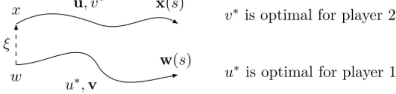
This suggest a way to find a control that allows the player to force the dynamics to stay in K, or close to it. Assume that the initial condition is in K and that the player will update his choice of control at discrete times s1, s2, . . . sN = 1. If at time sm the state
2.3. Differential games 17
zm:= (sm, ym) is in K, choose any u. If zm is outside of K, let wm denote a closest point
of zminto K and choose um such that
Èzm≠ wm,(sm, f(ym, um))Í Æ 0.
With this procedure one obtains the following.
Proposition 2.3.8. Consider a partition of [0, 1], denoted := {0 Æ t1, . . . , tN = 1} and
Î Î its mesh, i.e. Î Î := maxm<Ntm+1≠ tm. Let (K, ¯F) be viable, with F as in (2.5)
and f Lipschitz and bounded. Let (t1, x1) œ K.
There exists a piecewise constant control u (t) such that
˙x(t) = f(x(t), u (t)), x(t1) = x1
satisfies
d2K(x[t1, x1,u ](1)) Æ CÎ Î,
for a positive constant C independent of the .
We omit the proof as it is a corollary of the more general case with two players described in Chapter 4.
The construction described above is essentially the extremal aiming of Krasovskii and Subbotin [61] where player 2 is absent. It is also reminiscent of the construction in discrete time in the framework of Blackwell’s approachability, see Blackwell [14].
Quantitative case
Let us consider the case of a terminal payoff at time t = 1, i.e., an objective of the form g(x(1)).
For every initial condition (t1, x1) œ [0, 1] ◊ Rn, and a given u, we have a unique
trajectory, hence the following value function V(t1, x1) := sup
uœU(t1)
g(x[t1, x1,u](1))
is well defined.
The value function inherits the regularity of the payoff function. In particular, if g is Lipschitz, so is V(t, ·), for all t. We refer to Bardi and Capuzzo-Dolcetta [9, Chapter III, Prop. 3.1] for the proof.
The value function also satisfies the following crucial property.
Theorem 2.3.9. (Dynamic programming principle) Assume ¸, g are Lipschitz. Then, for
all (t, x) œ [0, 1] ◊ Rn and for all h > 0 :
V(t, x) = max
uœU{V(t + h, x[t, x, u](t + h))} .
At least heuristically, by a Taylor series expansion, one can deduce from the dynamic programming principle stated above that the value function should solve the following PDE:
ˆV
ˆt + maxuœU ÈÒxV, f(x, u)Í = 0 (2.6)
V(1, x) = g(x).
The partial differential equation (PDE) (2.6) is called Hamilton-Jacobi-Bellman equation. This PDE is important in optimal control theory because it provides necessary and sufficient optimality conditions. We refer to Bardi and Capuzzo-Dolcetta [9, Chapter III, Section 3] for a detailed description and proofs.
An important problem is that (2.6) fails to have solutions in the classical sense, even if the data of the problem (dynamics and payoff functions) is smooth. A significant breakthrough was achieved by Crandall and Lions [33], who introduced the definition of viscosity solutions, which will be recalled in Chapter 3.
Relation between the quantitative and qualitative case
Let us point out an important connection between qualitative and quantitative prob-lems.
Define v1:= V(t1, x1). Consider the target game with dynamics
(˙t(s), ˙x(s)) œ (1, F(x)), (t(0), x(0)) = (t1, x1), s œ [0, 1 ≠ t1] (2.7)
and target set Múµ [t1,1] ◊ Rn defined by:
Mú:= {(1, y) œ [0, 1] ◊ Rn | g(y) Ø v1}.
The link between the quantitative and qualitative game comes from the following propo-sition:
Proposition 2.3.10. The set
L(v1) := {(s, y) œ [t1,1] ◊ Rn | V(s, y) Ø v1}
is viable under the dynamics (2.7).
The intuition here is that the value function is constant along optimal trajectories: since there is no running payoff, it depends only on the terminal state, that is, the state at time t = 1. Hence, for any initial conditions in L(v1), there exists at least one trajectory
that remains there (e.g. an optimal trajectory) and leads to a terminal state in Mú.
An important consequence of this fact is that solving the target problem described above and using the construction of Proposition 2.3.8 we obtain an explicit method to derive ‘≠optimal strategies. We omit this construction here, but in Chapter 4 we describe in more detail the extension of this approach to the case of two players, zero sum games.
2.3.3 Two players
Qualitative case
We do not cover target games in detail in this thesis, but let us make some remarks. As it was pointed out before, the main complication in continuous time games comes from the fact that there is no canonical information structure. Let us describe briefly some of the information structures that have been proposed in the literature.
As an early example of alternative theorems for two players, let us mention the work of B.N. Pöeni nyj [79], who studies the target game with a different class of strategies
2.3. Differential games 19 Definition 2.3.11. (‘-strategies) We say the players are using ‘-strategies in the target game if the game is played as follows:
i) Both players know (t1, x1).
ii) player 2 chooses ‘1 >0 and informs player 1 of the control function v1 that he
will use in the interval [t1, t1+ ‘1].
iii) Using this information, player 1 chooses his control function.
iv) At time t1+ ‘1, the new state is announced and the situation is repeated, with
player 2 choosing ‘2.
Under this information structure, several examples of alternative theorems are pro-posed in [79], under different assumptions on the target set and the dynamics. However, in this theory no explicit connection with the quantitative case is made.
Krasovskii and Subbotin introduce the extremal aiming method [61] for target games. The description of this method motivates the work in Chapter 4. They use positional strategies, which are limits of piecewise constant motions. In general, the control func-tions originating from this procedure are not regular enough to obtain solufunc-tions in the Carathéodory sense. Thus, as in Pöeni nyj’s approach, their construction provides infor-mation of an approximated game only.
In order to solve the target game exactly, Cardaliaguet [21] considers instead non anticipating strategies which are defined later in Chapter 3 and establishes an alternative theorem. Note that this is an important advance with respect to the other approaches, since it allows us to solve the target game exactly, instead of an approximate version. Quantitative case
As we did for the target game, we need first to specify which information is available to the players and how are they allowed to interact. Different information patterns and strategies have been proposed in the literature, we refer to Bardi and Capuzzo-Dolcetta [9, Chapter VIII].
A common feature of these different notions is that they allow to reduce the problem to study a certain system of PDE’s. For the finite horizon game with ¸ © 0, these PDE’s are:
ˆw≠
ˆt (t, x) + supuœUvinfœV
+
f(x, u, v), Òxw≠(t, x), = 0 (2.8a)
ˆw+
ˆt (t, x) + infvœVusupœU
e
f(x, u, v), Òxw+(t, x)
f
= 0 (2.8b)
with boundary conditions w≠(1, x) = w+(1, x) = g(x).
Although the above relations were heuristically derived by Isaacs’ [58, Section 4.2], the connection between PDE’s and differential games was first made explicit in the framework of viscosity solutions [33] by Evans and Souganidis [36]. As pointed out by Lions in the introduction of the book [67], the study of these equations was a motivation to introduce the definition of viscosity solutions.
Note that under the following condition, called Isaacs’ condition sup
uœUvinfœV Èf(x, u, v), pÍ = infvœV supuœUÈf(x, u, v), pÍ
holds for all x, p œ Rn, there is only one equation, called Hamilton-Jacobi-Isaacs
Let us remark that this condition is conceptually very strong. It imposes the existence of the value of a family of games in pure strategies, which denies the important role of randomization in game theory, as pointed out in von Neumann’s remark above. In Chapter 3 we propose a way to avoid Isaacs’ condition, inspired from Fleming [38]. A different approach to introduce randomized strategies in differential games and hence avoid Isaacs’ condition has been proposed by Buckdahn, Li and Quincampoix [18].
Krasovskii and Subbotin applied their method to a suitable target set to establish the existence of the value for differential games with finite horizon and terminal payoff using an explicit description of ‘≠optimal strategies. The material of Chapter 4 is inspired from their construction, which allows to establish the existence and characterization of the value function. Later, Subbotin [97] proposes a notion of generalized solutions, called minimax solutions and characterizes the value function as the unique minimax solution of the HJI equation. We establish the equivalence of minimax solutions for HJI equations with the standard machinery of viscosity solutions in Chapter 5.
2.4 Discrete time mean field games
Let us briefly comment on some related (and important) previous work on games with a continuum of players before moving on to the framework of mean field games, to which our contributions are more closely related.
2.4.1 Games with a continuum of players
As pointed out in Section 2.2, we are interested in modelling situations with a "large" number of identical agents. This statement is ill-defined, but it could mean either of the three following situations:
1. Games with a continuum of agents per se.
2. Convergence, in a suitable sense, of a sequence of games with atomic players to a non atomic limit game.
3. Use the limit non atomic game to compute ‘≠optimal equilibria for the atomic game.
On the first situation, let us mention the pioneering work of Aumann [6]. One mo-tivation for introducing games with a continuum of agents is an important concept in economics, perfect competition. The essential idea of this notion is that there are many agents whose individual influence on the economy (e.g. for affecting prices) is negligible. Thus, following [6], the natural way to study economies with perfect competition is to consider non atomic agents. The introduction of this idea allows Aumann [6] to solve a long standing conjecture in economics.
Later, Mas-Colell [72] introduced the notion of distributional equilibrium for a one shot game with a continuum of players, building on results of Schmeidler [86]. The definition of distributional equilibrium is recalled later in Chapter 6. Let us refer also to Milgrom and Weber [76] were several existence results of Nash equilibrium are established for games with incomplete information where the set of types is a continuum.
The references cited above concern one shot games only. In dynamic games, let us mention the extension of the model of Mas-Colell by Jovanovic and Rosenthal [59] for discrete time stochastic games, which is also introduced in Chapter 6. Later, Lasry and Lions [64, 65, 66] and Huang, Caines and Malhamé [56, 57] introduced the mean field games theory, which studies non atomic dynamic games in continuous time.
2.4. Discrete time mean field games 21 The idea of using a continuum of players is also present in the literature on congestion games, which goes back to Wardrop [106] and Smith [89]. We refer to Wan [104, 105] for an extensive survey of this literature. Games with a continuum of players have also been introduced in the framework of population games by Hamilton [51] and Maynard Smith [73].
As for the convergence of equilibria of games with finitely many players to an equilib-rium of a non atomic game, an early example is the work of Haurie and Marcotte [52] in the framework of congestion games and Sandholm [85] for potential games.
In the framework of mean field games the convergence of the sequence of Nash equilibria of the N player games has been established by Lasry and Lions [64] for games with an ergodic payoff (see also Feleqi [37] for a detailed proof) and by Bardi [8] for linear quadratic mean field games.
Results of a similar flavour, based on stochastic approximation techniques, have been obtained by Benaïm and Weibull [10] for population games and by Gast, Gaujal and Le Boudec [44] for games with a centralized controller. In the stochastic approximation framework, the idea is to approximate the path of a Markov chain by a deterministic trajectory given by a suitable ordinary differential equation. The assumption these models have in common is that the probability that the relevant state variable in the N player game changes between two consecutive stages of the game goes to zero as N goes to infinity.
Our interest is more on the third situation: constructing an approximate Nash equilib-ria via suitably defined limit objects. In this sense, our contribution is closer to the work of Huang, Caines and Malhamé [57].
2.4.2 Continuous time mean field games
Mean field games have been introduced independently by Huang, Caines and Malhamé [56, 57] and by Lasry and Lions [64, 65, 66] and have received considerable attention in the literature. The aim of mean field games theory is to model situations with a large number of identical agents. Their distinctive feature is the backward-forward structure: each player anticipates a certain behavior of the other players and computes his own optimal behavior; if the observed aggregate behavior is consistent with the prediction, the players are said to be in a mean field game equilibrium. Precise definitions will be given in Chapter 6.
The following example is borrowed from Cardaliaguet’s notes on mean field games [20, p.2]:
Example 2.4.1. Let us consider first N players in Rd. The random position of player i
at time t is given by
dXti= –itdt+
Ô 2dBi
t
Each player i aims to minimize the cost:
⁄ T t 1 2|–is|2+ F (m≠is,N)ds + g(x i T, m≠iT,N) where m≠i s,N := N1≠1 q j”=i”xjs.
Heuristically, if one takes the limit as N æ +Œ, one obtains the following backward-forward system of coupled PDE’s:

![Figure 4.1.3 – Distance to a set W µ [t 0 , 1] ◊ R n satisfying P1 and P2.](https://thumb-eu.123doks.com/thumbv2/123doknet/2328958.31185/63.892.314.576.152.297/figure-distance-set-w-r-satisfying-p.webp)