Publisher’s version / Version de l'éditeur: Technical Report, CHC-TR-009, 2003-03
READ THESE TERMS AND CONDITIONS CAREFULLY BEFORE USING THIS WEBSITE.
https://nrc-publications.canada.ca/eng/copyright
Vous avez des questions? Nous pouvons vous aider. Pour communiquer directement avec un auteur, consultez la
première page de la revue dans laquelle son article a été publié afin de trouver ses coordonnées. Si vous n’arrivez pas à les repérer, communiquez avec nous à [email protected].
Questions? Contact the NRC Publications Archive team at
[email protected]. If you wish to email the authors directly, please see the first page of the publication for their contact information.
Archives des publications du CNRC
For the publisher’s version, please access the DOI link below./ Pour consulter la version de l’éditeur, utilisez le lien DOI ci-dessous.
https://doi.org/10.4224/12340935
Access and use of this website and the material on it are subject to the Terms and Conditions set forth at Ice decay boundaries for the ice regime system : Recommendations from a scientific analysis
Timco, G. W.; Johnston, M.
https://publications-cnrc.canada.ca/fra/droits
L’accès à ce site Web et l’utilisation de son contenu sont assujettis aux conditions présentées dans le site
LISEZ CES CONDITIONS ATTENTIVEMENT AVANT D’UTILISER CE SITE WEB.
NRC Publications Record / Notice d'Archives des publications de CNRC:
https://nrc-publications.canada.ca/eng/view/object/?id=de112647-e2f7-4f3a-a5f5-43e43638f192 https://publications-cnrc.canada.ca/fra/voir/objet/?id=de112647-e2f7-4f3a-a5f5-43e43638f192
TP 14096 E
Ice Decay Boundaries for the Ice Regime System:
Recommendations from a Scientific Analysis
G.W. Timco and M. Johnston
Sept Oct Nov Dec Jan Feb Mar Apr May June July Aug
0.0 0.2 0.4 0.6 0.8 1.0 1.2 No rm a lized St re n g th -40 -30 -20 -10 0 10 A ir T e m p e ra tu re (C ) early July 10% late-June 15-20% early-June 50% mid-May 70%
decay bonus decay bonus
Air Temperature
Technical Report CHC-TR-009
March 2003
TP 14096 E
Ice Decay Boundaries for the Ice Regime System:
Recommendations from a Scientific Analysis
G.W. Timco and M. Johnston Canadian Hydraulics Centre National Research Council of Canada
Ottawa, Ont. K1A 0R6 Canada
Technical Report CHC-TR-009
ABSTRACT
The Canadian Ice Regime System takes into account the decay of sea ice by allowing the addition of +1 to the Ice Multiplier for ice that is deemed to be decayed. The AIRSS definition of decay relates to the surface properties of the ice such that decayed ice is defined as ice that has thaw holes or is at the “rotten” stage. This report examines this approach based on an analysis of the strength of first-year sea ice, second-year sea ice, multi-year sea ice, and the damage statistics for Arctic vessels. The analysis shows that there is no quantitative scientific basis for the current AIRSS approach of taking into account the decay of sea ice in the Ice Regime System. The analysis further shows that the decay of sea ice can be quantified in a meaningful manner. The report provides a detailed discussion of the analysis with recommendations for modifying AIRSS to account for the decay of sea ice.
RÉSUMÉ
Le Système des régimes de glaces du Canada tient compte de la décroissance de la glace de mer en permettant l’ajout de +1 au Coefficient multiplicateur pour la glace jugée en décroissance. Dans le SRGNA, la définition de la décroissance réfère aux propriétés de la surface de la glace et la glace en décroissance est décrite comme présentant des trous de fonte ou se situant au stade de glace «pourrie». Dans ce rapport on examine cette approche en fonction d’une analyse de la résistance de la glace de mer de première année, de la glace de mer de deuxième année, de la glace de mer de plusieurs années et de statistiques sur les dommages causés aux navires arctiques. L’analyse montre que l’actuelle approche préconisée dans le SRGNA pour tenir compte de la décroissance de la glace de mer dans le Système des régimes de glaces n’a aucun fondement scientifique quantitatif. Elle montre en outre que la décroissance de la glace de mer peut être quantifiée de manière sensée. Le rapport comprend une discussion détaillée de l’analyse et des recommandations de modification du SRGNA permettant de tenir compte de la décroissance de la glace de mer.
TABLE OF CONTENTS ABSTRACT... 1 RÉSUMÉ ... 1 TABLE OF CONTENTS... 3 LIST OF FIGURES ... 4 LIST OF TABLES... 4 1.0 INTRODUCTION ... 5
2.0 SHIP DAMAGE IN THE CANADIAN ARCTIC ... 8
3.0 FIRST-YEAR SEA ICE ... 10
3.1 AIRSS Decay Bonus for Decayed First-Year Sea Ice... 10
3.2 Growth of Sea Ice ... 10
3.3 Ice Salinity ... 11
3.4 Brine Volume and Total Porosity ... 11
3.5 Flexural Strength... 13
3.6 Internal Processes within Sea Ice ... 14
3.7 Changes in Flexural Strength: Case Study ... 15
3.8 Ice Borehole Strength... 17
3.9 Decay Process in First-Year Sea Ice ... 21
3.10 Recommendations for the Decay Bonus for First-Year Ice... 22
4.0 SECOND-YEAR ICE ... 26
4.1 AIRSS Decay Bonus for Decayed Second-Year Sea Ice... 26
4.2 Strength of Second-Year Ice... 26
4.3 Recommendations for the Decay Bonus for Second-Year Ice... 28
5.0 MULTI-YEAR ICE... 30
5.1 AIRSS Decay Bonus for Decayed Multi-Year Sea Ice ... 30
5.2 Strength of Multi-year Ice ... 30
5.3 Decay Process in Multi-year Ice ... 32
5.4 Recommendations for the Decay Bonus for Multi-Year Ice ... 33
6.0 SUMMARY AND RECOMMENDATIONS... 34
7.0 ACKNOWLEDGEMENTS ... 35
LIST OF FIGURES
Figure 1: Vessel traffic in the Canadian Arctic by month for the 1996 calendar year (data from Mariport Inc.) ... 8 Figure 2: Histogram showing the number of damage events in the Arctic for each month
... 9 Figure 3: Ice salinity versus ice thickness for cold first-year sea ice ... 12 Figure 4: Flexural strength versus the square root of the brine volume for first-year sea
ice... 14 Figure 5: Ice thickness and air temperature for the Resolute region in the Canadian
Arctic... 15 Figure 6: Brine Volume and flexural strength calculated for the Resolute region from
the data input from Figure 5... 16 Figure 7: Photograph of the borehole jack ... 17 Figure 8: Photograph of the borehole jack in the ice. ... 18 Figure 9: First-year ice sites sampled during 2002 season (January 2002 RADARSAT
image courtesy of CIS) ... 19 Figure 10: Depth dependence of the borehole strength during the decay of first-year sea
ice from June 14 (JD165) to August 11 (JD223). ... 20 Figure 11: Borehole strength versus the time of year for first-year sea ice. Note the rapid decrease in strength during the spring. ... 21 Figure 12: Comparison of normalized ice borehole strength and calculated flexural
strength. ... 22 Figure 13: Relationship between ice strength and air temperature throughout the year
for the Resolute region. The time-frame where the decay bonus would be applied for this region is shown at the bottom of the figure. ... 23 Figure 14: CIS Ice Strength Chart for July 8, 2002. Note that most of the ice in this
region has strength between 10% to 15% of its mid-winter strength. ... 25 Figure 15: Photograph showing smooth surface of second-year ice ... 26 Figure 16: Photograph showing decayed second-year ice ... 27 Figure 17: Ice Conditions across Mould Bay in March-April 1983 (after Bjerkelund et
al., 1985)... 27 Figure 18: Borehole jack strength as a function of ice temperature, old ice ... 31 Figure 19: Comparison of first-year, second-year and multi-year borehole strength
during the decay season... 32
LIST OF TABLES
Ice Decay Boundaries for the Ice Regime System:
Recommendations from a Scientific Analysis
1.0 INTRODUCTION
Navigation in Canadian waters north of 60°N latitude is regulated by the Arctic Shipping Pollution Prevention Regulations (ASPPR). These regulations include the date Table in Schedule VIII and the Shipping Safety Control Zones Order, made under the Arctic Waters Pollution Prevention Act. Both of these are combined to form the “Zone/Date System” matrix that gives entry and exit dates for various ship types and classes. It is a rigid system with little room for exceptions. It is based on the premise that nature consistently follows a regular pattern year after year.
Transport Canada, in consultation with stakeholders, has made extensive revisions to the Arctic Shipping Pollution Prevention Regulations (ASPPR 1989; Canadian Gazette 1996; AIRSS 1996). These changes, introduced only outside the zone-date system, were designed to reduce the risk of structural damage in ships which could lead to the release of pollution into the environment, yet provide the necessary flexibility to shipowners by making use of actual ice conditions, as seen by the Master. In this new system, an "Ice Regime", which is a region of generally consistent ice conditions, is defined at the time the vessel enters that specific geographic region, or it is defined in advance for planning and design purposes. The Arctic Ice Regime Shipping System (AIRSS) is based on a simple arithmetic calculation that produces an “Ice Numeral” that combines the ice regime and the vessel’s ability to navigate safely in that region. The Ice Numeral (IN) is based on the quantity of hazardous ice with respect to the ASPPR classification of the vessel (see Table 1). The Ice Numeral is calculated from
IN =[CaxIMa] + [CbxIMb] +.... (1) where
IN = Ice Numeral
Ca = Concentration in tenths of ice type “a”
IMa = Ice Multiplier for ice type “a” (from Table 1)
The term on the right hand side of the equation (a, b, c, etc.) is repeated for as many ice types as may be present, including open water. The values of the Ice Multipliers are adjusted to take into account the decay or ridging of the ice by respectively adding or subtracting a correction of 1 to the Ice Multiplier (see Table 1).
The Ice Numeral is therefore unique to the particular ice regime and ship operating within its boundaries.
Table 1 Table of Ice Multipliers for AIRSS
Type E Type D Type C Type B Type A CAC 4 CAC 3
Old / Multi-Year Ice……….. (MY) -4 -4 -4 -4 -4 -3 -1
Second Year Ice……….. (SY) -4 -4 -4 -4 -3 -2 1
Thick First Year Ice………. (TFY) > 120 cm -3 -3 -3 -2 -1 1 2
Medium First Year Ice…………. (MFY) 70-120 cm -2 -2 -2 -1 1 2 2
Thin First Year Ice………. Thin First Year Ice - 2nd Stage
(FY) 30-70 cm
50-70 cm -1 -1 -1 1 2 2 2
Thin First Year Ice - 1st Stage 30-50 cm -1 -1 1 1 2 2 2
Grey-White Ice………. (GW) 15-30 cm -1 1 1 1 2 2 2
Grey Ice………. (G) 10-15 cm 1 2 2 2 2 2 2
Nilas, Ice Rind < 10 cm 2 2 2 2 2 2 2
New Ice……….. (N) < 10 cm " " " " " " "
Brash (ice fragments < 2 m across) " " " " " " "
Bergy Water " " " " " " "
Open Water " " " " " " "
Ice Decay : Add 1 to the IM for MY, SY, TFY, MFY ice if the ice has Thaw Holes or is Rotten.
Ice Types Ice Multipliers
Ice Roughness : Subtract 1 from the IM if the floes are more than 3/10s ridged and the overall ice concentration is greater than 6/10s
The ASPPR deals with vessels that are designed to operate in severe ice conditions for transit and icebreaking (CAC class) as well as vessels designed to operate in more moderate first-year ice conditions (Type vessels). The System determines whether or not a given vessel should proceed through that particular ice regime. If the Ice Numeral is negative, the ship is
not allowed to proceed. However, if the Ice Numeral is zero or positive, the ship is allowed to
proceed into the ice regime. Responsibility to plan the route, identify the ice, and carry out this numeric calculation rests with the Ice Navigator who could be the Master or Officer of the Watch. Due care and attention of the mariner, including avoidance of hazards, is vital to the successful application of the Ice Regime System. Authority by the Regulator (Pollution Prevention Officer) to direct ships in danger, or during an emergency, remains unchanged.
At the present time, there is only partial application of the ice regime system, exclusively outside of the “zone-date” system.
Credibility of the new system has wide implications, not only for ship safety and pollution prevention, but also in lowering ship insurance rates and predicting ship performance. Therefore, there is a need to establish a scientific basis for the system. To this end, Transport Canada approached the Canadian Hydraulics Centre of the National Research Council of Canada (CHC/NRC) in Ottawa to assist them in developing a methodology for establishing a scientific basis for AIRSS. Considerable progress has been made in addressing the scientific basis (see Timco and Kubat (2001) for a recent update).
One important aspect of the Ice Regime System (IRS) is the decay of the sea ice. As noted in Table 1, an additional integer value is added to the Ice Multiplier if specific types of sea ice are decayed. The IRS allows the addition of one to the Ice Multiplier if the multi-year ice, second-year ice, thick and medium first-year ice is decayed. No allowance is made for decay
in thinner ice. This modification can significantly increase the Ice Numeral for decayed ice regimes.
This modification for decay was originally done on an “ad hoc” basis with no scientific evidence established for it. Further, there is no accepted definition of ice decay. Because of this, Transport Canada has asked the CHC/NRC to review this question. An initial study of this issue was discussed in Timco et al. (2002). In the present report, the previous work is extended. Ship damage events in the Arctic are reviewed to provide some insight into the time of year when damage events occur. The properties and strength of sea ice are reviewed with an eye towards the decay process. This is done for first-year sea ice, second-year ice and multi-year ice. The report provides key recommendations for an approach that could be taken for considering the decay of sea ice in the Ice Regime System.
2.0 SHIP DAMAGE IN THE CANADIAN ARCTIC
As a first step, it is instructive to understand the volume and timing of vessel traffic in the Arctic. The majority of vessel traffic occurs during the summer months. This traffic is primarily comprised of commercial shipping for transporting goods to the Arctic, removal of natural resources from mines, fishing vessels, tour boat operations and government vessels. In the 1970s and 1980s there also was some activity in the Beaufort Sea related to offshore oil and gas exploration. At the present time, this Beaufort activity has stopped. To quantify the volume of traffic, use was made of a database developed by Mariport Inc. They have compiled a list of vessel traffic in the Arctic for several years. For the present analysis, the data from 1996 was used. In this year, Mariport reported that there were 59 different vessels in the Canadian Arctic. These data were analysed to count the number of different vessels that were in the Arctic during each month of the 1996 calendar year. Figure 1 shows that there is some limited shipping in June and July, but the majority of traffic takes place during August and September. Sept Oct Aug July June May Apr Mar Feb Nov Jan Dec 0 10 20 30 40 50 Nu mb e r o f V ess el s 1996 Data
Figure 1: Vessel traffic in the Canadian Arctic by month for the 1996 calendar year (data from Mariport Inc.)
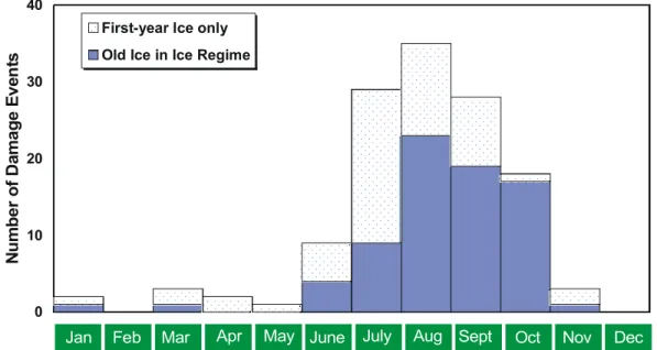
The Canadian Hydraulics Centre has developed a database related to vessel damage due to ice, as part of their work to put the Ice Regime System on a scientific basis (Timco and Kubat, 2001). This database contains over 1500 Events related to both damage and no-damage Events of ships in ice-covered waters. The database was queried to extract the information related to vessel damage due to ice. The query included all types of damage (not just hull-related damage). The data was filtered to look at regions with latitude north of 57° and includes approximately 20 years of damage statistics. The vast majority of the damage Events relates to the Canadian Arctic, but there are also a few Events in the American Arctic and in the Baltic Sea. Figure 2 shows a histogram of the results. The data have been further separated based on the presence of old or multi-year ice at the time of the vessel damage.
Several observations can be made from this figure:
The shape of the histogram is very similar to Figure 1; i.e. there are more damage events with more vessel traffic.
The largest number of damage events occurred in August, with slightly fewer damage Events in both July and September.
In July, there are a large number of Events in which only first-year ice is present. Between August and October, there are a similar number of damage events with multi-year ice present, but a decreasing number with only first-year ice present.
Sept Oct Aug July June May Apr Mar Feb Nov Jan Dec 0 10 20 30 40 Nu m b e r o f D a m a g e E v e n ts
First-year Ice only Old Ice in Ice Regime
Figure 2: Histogram showing the number of damage events in the Arctic for each month. The data is based on approximately 20 years of information.
3.0 FIRST-YEAR SEA ICE
3.1 AIRSS Decay Bonus for Decayed First-Year Sea Ice
The AIRSS Regulatory Standard (AIRSS, 1996) specifies that a bonus of +1 may be applied to the Ice Multiplier of Thick and Medium First-Year ice if the ice is Decayed. The Standards define decayed ice as ice that has thaw holes formed, or is rotten ice. Basically this bonus takes into account the fact that first-year sea ice is considerably weaker in strength than sea ice in the winter. In the following sections, some background information is given on the properties, growth and decay of first-year sea ice. Following that, a discussion and recommendations on the decay bonus for first-year sea ice is given.
3.2 Growth of Sea Ice
Sea ice is a complex material that is composed of solid ice, brine, air and, depending upon the temperature, solid salts. Ice growth mechanisms can produce several different grain structures, depending upon the prevailing conditions. The details of the ice microstructure influence significantly the mechanical and physical properties of the ice. When the ice grows, it traps some of the salt that is present in the seawater. The amount of salt that is trapped in the growing ice sheet is affected by several factors. Typically first-year sea ice has salinity in the range of 4 to 6 parts per thousand (‰) salt. This is lower than the salinity of seawater, which is typically 35 ‰. The brine, air and solid salts are usually trapped at sub-grain boundaries between a mostly pure ice lattice. Also, because a temperature gradient exists, the upper surface temperature is close to the ambient air temperature, and the lower surface temperature is at the freezing point (usually -1.8°C for sea ice). Because there are a number of salts in the ice, the phase relationship with temperature is multifarious (see e.g., Weeks and Ackley 1982). All of these factors make understanding and charactering sea ice extremely difficult.
The surface appearance of first-year sea ice changes as the ice gets thicker. The Stages of Development of the ice is categorized as follows (MANICE, 2002):
New (N) (less than 10 cm thick) - Sea ice that is in early stages of formation. This ice is less
than 10 cm thick and in small platelets or lumps, or ice in a soupy-looking layer. New ice is usually subdivided into frazil, grease ice, slush or shuga.
Nilas (NI) (less than 10 cm thick) - A thin elastic crust of floating ice that easily bends from
waves and swells. It has a matte surface appearance.
Young Ice (YN) (10 to 30 cm thick) - Young ice is subdivided into the following sub-stages: Grey (G) - Young ice, 10 to 15 cm thick, that is less elastic than Nilas. It often breaks from
swells.
Grey-white (GW) - Young ice, 15 to 30 cm thick.
Thin First-year Ice (FY) (30 to 70 cm thick) - Sea ice that grows from Young Ice and is 30
to 70 cm thick. This is separated into: Stage 1 (30 to 50 cm thick); and Stage 2 (50 to 70 cm thick).
Medium First-year Ice (MFY) (70 to 120 cm thick) - Sea ice that is 70 to 120 cm thick.
3.3 Ice Salinity
For sea ice, the salinity (Si) is usually expressed as the fraction by weight of the salts
contained in a unit mass. It is usually quoted as a ratio of grams per kilogram of seawater, that is, in parts per thousand (‰ or ppt). In sea ice there is usually some salinity variation with depth in the ice sheet. This depth dependence of the salinity changes throughout the winter as the salt within the ice migrates downward through the ice. There can be, however, marked salinity variations even within a small sample. In many cases, therefore, the average value of a salinity profile is used as a first approximation of salinity for an ice sheet.
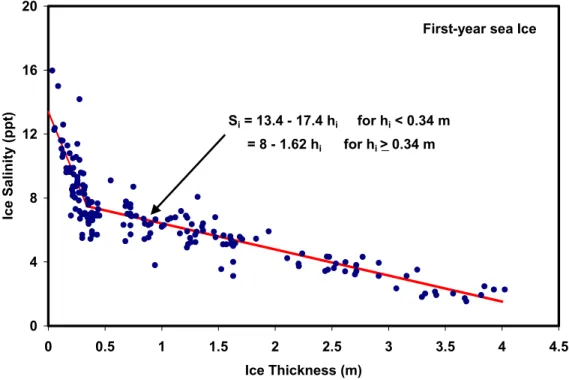
In collating information on sea ice from a wide number of sources, Cox and Weeks (1974) found that the average salinity of a cold ice sheet could be related to the thickness of the ice (hi). Figure 3 shows a plot of the average ice salinity (Si) versus ice thickness for a large
number of measurements on sea ice sampled during the growth season. The graph gives the original data of Cox and Weeks along with some more recent data from Frederking and Timco, Sinha and Nakawo, and Frederking. The data were collected from cores from all parts of the Arctic including the Beaufort Sea, Bering Sea, Labrador, Eclipse Sound and Strathcona Sound. From Figure 3 it appears that a reasonable representation of the ice salinity for a given ice thickness hi can be expressed as (from Timco and Frederking 1990):
; 34 . 0 4 . 17 4 . 13 h for h m Si = − i i ≤ ; 34 . 0 62 . 1 0 . 8 h for h m Si = − i i ≥ (2)
This approach assumes that there is no salinity variation with depth through the ice sheet, which is a reasonable first approximation for sea ice. Equation (2) gives the average salinity of sea ice as a function of the ice thickness. As evidenced in Figure 3, there is a good fit of the equations to the data. The change in salinity with thickness reflects the drainage of the brine during the year, and the fact that slower growth rates trap less salt in the ice sheet. With thicker ice, the growth rate is substantially lower than that for a thin (usually snowless) ice sheet in the early winter. All of these factors affect the strength of the ice.
3.4 Brine Volume and Total Porosity
Historically sea ice has been analyzed in terms of the "brine volume" in the ice. The brine volume represents the amount of liquid brine in the host ice matrix. The determination of the brine volume integrates the influence of both temperature and salinity. The brine volume (νb) of the ice is related to the temperature (Ti ) of the ice, the salinity (Si ) of the ice and the types
of salts present. For sea ice, the brine volume can be determined from the Frankenstein and Garner (1967) Equation: + = 49.185 0.532 i i b T S υ (3)
) ( / F1 T Si i b ρ υ = (4)
where ρi is the bulk ice density, and
F1(Ti ) = - 4.732 - 22.45 Ti - 0.6397 Ti2 - 0.01074 Ti3
for - 2 ≥ Ti ≥ - 22.9
= 9899 + 1309 Ti + 55.27 Ti2 + 0.716 Ti3
for - 22.9 ≥ Ti ≥ - 30
Although the latter is more accurate, the former provides a reasonable estimate of the brine volume. The brine volume is usually quoted in terms of the volume in parts per thousand, similar to the salinity. Alternatively, it can be expressed as a volume fraction. (For example, a brine volume of 20 ‰ is equivalent to a brine volume fraction of 0.020).
0 4 8 12 16 20 0 0.5 1 1.5 2 2.5 3 3.5 4 4.5 Ice Thickness (m) Ice Salinity (ppt) Si = 13.4 - 17.4 hi for hi < 0.34 m = 8 - 1.62 hi for hi > 0.34 m
First-year sea Ice
Figure 3: Ice salinity versus ice thickness for cold first-year sea ice
Knowledge of the brine volume for sea ice is useful on its own. However, in addition to the liquid brine in the ice, air is present in the ice. In certain instances (especially where brine drainage occurs) the air volume can be significant. For this reason it is usually better to express the porosity of the ice as the total porosity (i.e. brine plus air). For this, the total porosity (νT) of the ice is expressed as
where νb is the relative brine volume and νa is the relative air volume. Cox and Weeks (1982) developed equations to calculate the total porosity. To do this, the bulk ice density must be known accurately. Since this is a property that is not usually known due to the difficulty of an accurate measurement, the following discussion will be related only to the brine volume.
3.5 Flexural Strength
Several researchers have attempted to relate the strength of sea ice to the brine volume or total porosity of the ice. There is a good reason for this. It is generally assumed that as the total porosity in the ice increases, the strength should decrease since there is less "solid ice" that has to be broken. Timco and O’Brien (1994) have done the most comprehensive analysis of the flexural strength of ice. They compiled a database of over 2500 reported measurements on the flexural strength of freshwater ice and sea ice. For this data set, approximately 1000 tests were performed on sea ice. Timco and O’Brien (1994) showed that the data for first-year sea ice could be described by:
) * 88 . 5 ( exp 76 . 1 b f υ σ = − (6)
where σf is the flexural strength of the ice and the brine volume (νb) is expressed as a brine
volume fraction. This relationship is shown with the data in Figure 4.
Several observations can be made from this figure:
The value of 1.76 MPa for zero brine volume is in excellent agreement with the average strength (1.73 MPa) measured for freshwater ice.
The general scatter in the data increases with decreasing brine volume. This is a reflection of the fact that, at low brine volumes, the ice is much more brittle. The range of scatter approaches that measured for freshwater ice. This type of scatter is characteristic of a brittle material. It is natural scatter.
This equation is the most comprehensive equation for flexural strength to date. There have been a few other equations proposed to relate strength and brine volume but these have been based on substantially fewer data points, and data that extended over a very limited range. In other words, the other equations are valid over only a small brine volume range. The wider range of this equation represents these other equations very well in the ranges where they are valid.
The data for the equation was compiled from a large number of investigators, and from a variety of geographic locations, in both polar and temperate climates. Therefore it should be quite representative of the flexural strength of sea ice in most regions. The brine volume used to represent the ice beam for any test was taken to be the average brine volume, determined from the average temperature and salinity of the beam. Thus, to calculate the flexural strength, it is only necessary to know the average temperature and salinity of the ice.
0 0.5 1 1.5 2 0 0.1 0.2 0.3 0.4 0.5 0.6
Square Root of Brine Volume (νb) 1/2 Flexural St rengt h ( M Pa)
First-year Sea Ice
Average value for freshwater ice
σf = 1.76 exp [-5.88*sqrt(νb)]
Figure 4: Flexural strength versus the square root of the brine volume for first-year sea ice.
In summary, the fact that a very large number of data points have been used in this analysis, the excellent agreement with the flexural strength of freshwater ice at zero brine volume and the associated scatter comparable to freshwater ice, indicates this equation is a very good representation of the dependence of flexural strength of sea ice on the brine volume.
3.6 Internal Processes within Sea Ice
The information discussed above provides some insight into the internal processes within sea ice. During the mid-winter months, the air temperature is very low and the ice is cold. When the ice is cold, the majority of entrained salt is in the form of precipitated crystals within the brine pockets. As spring approaches, the air temperature progressively warms and the internal temperature of the ice increases. Increasing ice temperatures cause a phase change within the brine pockets whereby precipitated salts dissolve and enter solution. As the salts dissolve, ice melts along the walls of the brine pocket and the overall brine volume increases.
As the ice temperature warms, the ice becomes nearly isothermal. Brine pockets continue to increase in size and eventually interconnect to form large brine drainage channels within the ice. These channels provide a conduit for the liquid brine to “drain” out of the ice. Once the brine drainage channels form the ice salinity decreases rapidly. Ice that is isothermal and from which most of the salinity has drained is considered to be in an advanced state of decay. What does ice decay mean quantitatively in terms of the degradation in ice strength? To answer this, a natural starting point would be to calculate the flexural strength of the ice using the inverse relationship between ice strength and brine volume described in Equation 6. The following discussion focuses upon changes in the flexural strength of the ice during the decay season.
3.7 Changes in Flexural Strength: Case Study
It is possible to use this information to determine the flexural strength of first-year ice throughout its lifetime. As an example, the sea ice in the Resolute region in the Canadian Arctic will be discussed. To determine the flexural strength, it is necessary to know the brine volume of the ice. This can be determined if the ice salinity and ice temperature are known. Figure 3 shows the relationship between the salinity and ice thickness, so if the thickness is known, the salinity can be determined. Information on the ice thickness in the Resolute region can be found in Billelo (1980), who measured the ice thickness on first-year ice near Resolute from 1959 to 1972. To determine the ice temperature, a linear temperature profile was assumed for the ice with the bottom ice temperature of –1.8°C. The ice surface temperature (Ts) was determined from the relationship developed by Timco and Frederking (1990):
Ts = Ta for –2 ≥ Ta ≥ -10
Ts = 0.6 Ta – 4 for Ta< -10 (7)
where Ta is the air temperature in °C. For this analysis, the air temperature at Resolute was
obtained from the Canadian Ice Service. Using this approach, the flexural strength can be calculated based upon only the ice thickness and air temperature.
Figure 5 presents a graph of the air temperature and ice thickness at Resolute for a typical winter. In September, the air temperature is below 0°C and steadily decreases. The temperature reaches a low value of approximately -35°C in January to March. In April, the air temperature begins to rise and reaches 0°C in June. Corresponding to this change in temperature, the ice begins to grow in September and reaches a maximum thickness of approximately 1.8 m in mid-April. The ice begins to melt in early July. Once the melting begins, the decrease in ice thickness is quite rapid.
Sept Oct Nov Dec Jan Feb Mar Apr May June July Aug
-40 -30 -20 -10 0 10 A ir T e m p er a tu re (C ) -2.0 -1.5 -1.0 -0.5 0.0 Ic e T h ic k n ess (m ) Ice Thickness Air Temperature
Figure 5: Ice thickness and air temperature for the Resolute region in the Canadian Arctic.
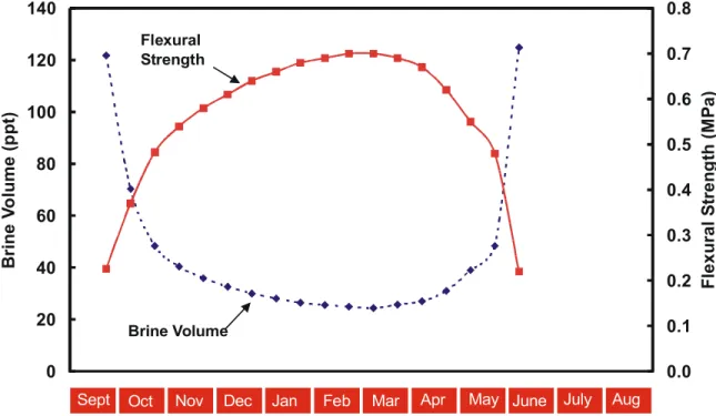
Figure 6 presents information on the corresponding brine volume and flexural strength for the conditions given in Figure 5. In September and October when the ice is forming, the brine volume is relatively high in the ice. As winter progresses, the air temperature decreases and the average ice salinity also decreases, with a resultant decrease in the brine volume. The figure shows that for most of the winter months, the brine volume in the ice is relatively constant at approximately 25 ‰. In spring, there is a steady increase in air temperature and solar radiation intensifies. When this occurs, the brine volume in the ice dramatically increases into an almost “runaway” condition in mid- to late June. The flexural strength is almost a mirror image of the brine volume. It is relatively low in the autumn when the ice is forming, and remains relatively constant throughout the winter months. In April, the strength of the ice begins to decrease rapidly such that by mid-June, the strength is considerably lower than the mid-winter strength. At this stage, the ice temperature is close to the melting point and the equations for calculating the brine volume are no longer valid. At the same time, the ice begins to decrease in thickness.
Sept Oct Nov Dec Jan Feb Mar Apr May June July Aug
0 20 40 60 80 100 120 140 Br in e V o lu m e( p p t) 0.0 0.1 0.2 0.3 0.4 0.5 0.6 0.7 0.8 Fl e x ur a l S tr e ng th (M P a ) Flexural Strength Brine Volume
Figure 6: Brine Volume and flexural strength calculated for the Resolute region from the data input from Figure 5.
In order to calculate the flexural strength of decaying sea ice, an equation would need to be developed to take into account the total porosity of the ice (Equation 5), rather than only the brine volume. Calculation of the total porosity requires reliable information about the density of the ice. The wide range of scatter in the reported densities of cold, winter sea ice (Timco and Frederking, 1996) illustrates the difficulty of obtaining accurate ice density measurements. It is considerably more difficult to measure accurately the density of warm sea ice. As a result, developing an equation that requires the total porosity as input is a formidable and at this time, an impossible task. Clearly, it becomes necessary to use other means to measure the strength of decaying sea ice. The most feasible means of determining
the strength of warm ice would be to avoid performing property measurements on an extracted ice core, i.e. to do the strength tests in situ. The borehole jack assembly fulfils that requirement.
3.8 Ice Borehole Strength
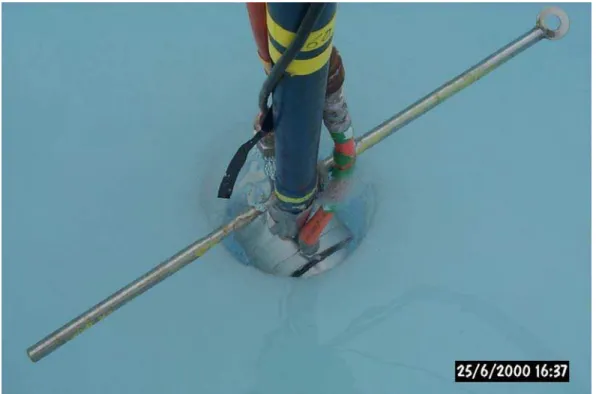
The borehole jack test has been used extensively to characterize the in situ strength of ice. The jack consists of a high-strength stainless-steel hydraulic cylinder with a double-acting piston (Figure 7) that pushes on the sidewalls of an augured hole in the ice (Masterson, 1996). Pressure is applied to the front and back load plates hydraulically by means of the piston located inside the jack body and activated by a pump at the surface of the ice. Oil is transferred from the pump to the piston by means of hydraulic high-pressure hose supplied with quick-disconnect couplings. Displacement is usually measured by using a linear, variable resistor (potentiometer) mounted inside the jack body and attached to the front plate. Resistance is related to displacement by a calibration curve and is measured at the surface by means of an ohms meter (multimeter) or on a chart recorder.
Figure 7: Photograph of the borehole jack
For a test, the jack is placed into an augured hole in the ice and lowered to the desired depth (see Figure 8). Hydraulic fluid is supplied to the jack and the pistons begin to exert pressure on the sidewalls of the ice. In this case, the principal stress is the applied plate pressure. Since the pressure is being applied to what is essentially the surface of a semi-infinite solid, the stresses are three-dimensional. At the beginning of the test, a bulb of crushed ice forms beneath the load plates as a result of surface unevenness and high local stress concentrations. The bulb continues to crush the surrounding ice as the applied pressure is increased until at some point it pushes out around the load plate and failure is reached. In many cases, the crushed ice never escapes from the bulb but the size of the bulb diameter grows larger and the
displacement increments increase exponentially. Some of the ice near the load plate recrystallizes from the high pressure. Large displacements are associated with this consolidation. By plotting pressure/displacement curves the “ultimate" or confined compressive strength of the ice can be determined since the curve approaches this value asymptotically (Masterson, 1996). Note that in contrast to the uni-axial strength tests, the stress conditions and stress-state for this test are very complex.
Figure 8: Photograph of the borehole jack in the ice.
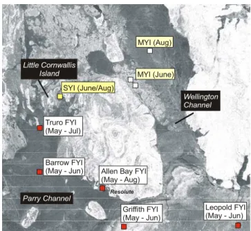
Three seasons of measurements have been conducted near Resolute, Cornwallis Island in the Canadian Arctic to investigate systematically the decay process in first-year sea ice. The first season, in 2000, focused upon level, landfast first year ice near Truro Island (74°14′N, 97°13′W), Nunavut. The success of the first season led to a second season of measurements on first year ice around Truro Island. The third season, in 2002, expanded the objectives: different areas of first year ice were sampled, as well as different types of sea ice. The programs began in May, when the ice was cold, and extended until June and July, when the snow cover had melted fully and the ice was beginning to ablate. Property measurements included snow depth, ice thickness, air and ice temperature and ice salinity. Figure 9 shows the location of the measurements in this program.
Truro (May - Jul)
FYI
Barrow FYI
(May - Jun) Allen Bay FYI (May - Aug) Griffith FYI (May - Jun) Resolute MYI (June) MYI (Aug) Parry Channel Wellington Channel SYI (June/Aug) Little Cornwallis Island Leopold FYI (May - Jun)
Figure 9: First-year ice sites sampled during 2002 season (January 2002 RADARSAT image courtesy of CIS)
Measuring the in situ, confined compressive strength of the ice (i.e. ice borehole strength) with a borehole jack was a significant component of the field programs. Strength measurements were obtained at least twice per week in the early season and more frequently as the season progressed. Each test day, depth profiles of the ice borehole strength were obtained throughout the full thickness of the ice for a total of three holes. Results from the different borehole jack tests were compared based upon the pressure at an indentor displacement of 3 mm (σ3mm).
Figure 10 shows the borehole strength as a function of depth in the ice sheet for six different days ranging from JD165 (June 14) to JD223 (August 11). These data were collected in Allen Bay in 2002, and show the changes in the ice strength as the ice decays. The data show that in the later part of June, the first year ice in Allen Bay was 1.83 to 1.88 m thick and had an ice borehole strength between 4.0 and 8.1 MPa. Ice in the upper and lower surfaces (depths 0.30 and 1.80 m) had half the strength of the ice interior. Strength in the ice interior was relatively constant (from 7.1 to 8.0 MPa) until the bottom ice was reached. When Allen Bay was revisited on 11 August (JD223), the first year ice was between 1.2 and 1.3 m thick and the ice borehole strength ranged from 3.1 to 4.5 MPa. Moreover, at that time, there was little difference in the strength at different depths. The reader is referred to Johnston et al. (2000), Johnston and Frederking (2001) and Johnston et al. (2003a) for a more thorough discussion of results from each season.
-2.1 -1.8 -1.5 -1.2 -0.9 -0.6 -0.3 0.0 0 2 4 6 8 10 12 14
Borehole Strength (MPa)
Depth in Ice Sheet (m)
Allen Bay JD165 JD168 JD171 JD175 JD207 JD223
Figure 10: Depth dependence of the borehole strength during the decay of first-year sea ice from June 14 (JD165) to August 11 (JD223).
Results from the borehole jack tests during the decay season were compared to published measurements made in the winter on first-year sea ice (Blanchet et al., 1997; Masterson et al., 1997). The Blanchet et al. (1997) data was used to extrapolate the borehole strength to mid-winter conditions resulting in a value of 33 MPa. Note that the Blanchet data was modified to allow a comparison to be made at a common loading rate (see Johnston et al. (2003a) for details).
The results from the three field programs are shown in Figure 11 along with the mid-winter borehole strength value. There is very good agreement in the strengths for all of the sites investigated. The figure shows that there is a dramatic decrease in the strength during the spring when air and ice temperatures begin to warm. The data shows that, by early July, the borehole strength is approximately 10% of the mid-winter strength. After the first week of July, the change in strength decreases and the strength is relatively constant during the remainder of the decay/melting of the ice.
0 5 10 15 20 25 30 35 50 100 150 200 250
Ice borehole strength (MPa)
2000_Truro 2001_Truro 2002_Truro 2002_Allen Bay 2002_Barrow 2002_Griffith 2002_Leopold
April May Jun Jul Aug Sep
Apr May Feb- Mar
mid-winter
Julian Day
Figure 11: Borehole strength versus the time of year for first-year sea ice. Note the rapid decrease in strength during the spring.
3.9 Decay Process in First-Year Sea Ice
As previously discussed, the flexural strength equation is not reliable for warm sea ice. In the temperature region where the flexural strength equation is not appropriate, borehole jack tests offer a feasible means of measuring the in situ confined compressive strength of the ice. Having demonstrated the feasibility of the borehole jack in measuring the strength of decaying ice, it is instructive to see how the in situ confined compressive strength relates to the flexural strength of the ice.
Figure 12 shows the calculated flexural strength and the measured borehole strength, both normalized to their mid-winter strengths. The trends of decreasing normalized strengths are in excellent agreement with one another. Both strengths show that in mid-May, the ice had about 60-70% of its winter strength. By early June, the ice had about 50% of its mid-winter strength. After the first week of June, only the borehole jack measurements provided information about the degradation in ice strength. Measurements showed that by the end of June, the ice had only 15 to 20% of its mid-winter strength. The ice strength was stable during the month of July, when only 10% of the mid-winter ice strength remained.
Sept Oct Nov Dec Jan Feb Mar Apr May June July Aug 0.0 0.2 0.4 0.6 0.8 1.0 1.2 N o rm aliz e d S tr e n g th
Measured Borehole Strength Calculated Flexural Strength
Based on Historical Ice Thickness Values Based on Actual Ice Thickness Values CHC Measured Values Blanchet et al. Measured Values
Figure 12: Comparison of normalized ice borehole strength and calculated flexural strength.
The correlation between the ice strength and air temperature is shown in Figure 13. Increasing air temperatures are the primary reason for the decrease in ice strength during the decay season. Once the air temperature warms to about –10°C, the majority of the internal salts within the ice have converted from the solid phase to the liquid phase, and the sea ice is no longer in its mid-winter state. After the ambient air temperatures rise above about –10°C, the brine pockets rapidly begin to increase in size, causing a decrease in ice strength. Figure 13 shows that the decrease in ice strength continues until early July, by which time the ice has about 10% of its mid-winter strength.
3.10 Recommendations for the Decay Bonus for First-Year Ice
The current Ice Regime System takes into account the large difference in strength between mid-winter ice and summer ice by introducing the “decay” of the sea ice. This is done by allowing the addition of +1 to the Ice Multipliers for Thick First-year and Medium First-year ice when the ice has “thaw holes” or is decayed to the “rotten” stage. This is a very qualitative approach. The definition of the rotten stage is not quantitatively well-defined (and it is not easily detectable). Further, as can be seen from Figure 12 and Figure 13, there is not an abrupt change in strength at any time – rather, there is a continual decrease in the strength of the ice once the air temperature begins to rise. This decrease in strength is directly related to the rise in the air temperature. The data show that the strength of the ice sheet has decreased to approximately 20% of its mid-winter strength when the mean ambient air temperature remains consistently above 0°C. Further, when the air temperature remains above 0°C for several weeks, the strength of the ice drops to approximately 10% of its mid-winter strength. This analysis provides a quantitative method for incorporating the difference in mid-winter and summer strength.
Sept Oct Nov Dec Jan Feb Mar Apr May June July Aug 0.0 0.2 0.4 0.6 0.8 1.0 1.2 No rm al iz ed S tr e n g th -40 -30 -20 -10 0 10 A ir T e m p e ra tu re (C ) early July 10% late-June 15-20% early-June 50% mid-May 70%
decay bonus decay bonus
Air Temperature
Figure 13: Relationship between ice strength and air temperature throughout the year for the Resolute region. The time-frame where the decay bonus would be applied for this region is shown at the bottom of the figure.
Measurement of air temperature is very easy. The present analysis has shown that this property can be directly related to the strength of first-year sea ice. This can be used as a means of defining the stage at which the summer bonus could be given to the Ice Multiplier for first-year sea ice.
When should the summer bonus be given? There are several aspects that must be considered for this. The data show that the strength of the ice is approximately 20% of the mid-winter strength once the air maintains a temperature of 0°C for a few days. This is a result of a gradual increase in temperature during the spring with a resultant decrease in strength. Does this value seem reasonable to take for the summer bonus? For the Arctic, above zero temperatures occur typically at the end of June. An examination of the ship traffic and damage statistics (see Figure 1 and Figure 2) shows that there are a large number of damage incidents during July when the vessel traffic is still relatively low. Thus, a value of 20% of mid-winter strength is too high. If a value of 10% of mid-winter strength were used, this would typically occur in mid-July on the Resolute region; i.e. one month with ambient air temperatures above 0°C. This strength of the ice at that time should not present any potential hazard for ice-strengthened vessels. Further, the ice at this time has thinned considerably from its mid-winter thickness (Figure 5). Thus, it is recommended that summer decay bonus can be
applied if the CIS Ice Strength Charts indicate that the ice strength is 10% or less of the mid-winter strength. If this information is not available, the decay bonus can be applied if observations show that the ice has decayed to the rotten stage (thaw holes throughout the full-thickness of ice).
Recently, the Canadian Ice Service has developed a new product to provide direct information on the strength of level first-year sea ice. Collaborative research in developing this product has taken place between the CIS and the CHC with very promising results (Gauthier et al., 2002; Langlois et al, 2003; Johnston and Timco, 2003). Figure 14 shows an example of one of the CIS Ice Strength Charts that were produced during the spring of 2002 for the Resolute region. This product can be used to determine where and when the ice decay bonus can be applied. If this information is not available, the current definition of ice decay (thaw holes or rotten) could be used to determine if the decay bonus should be applied. A recent study (Timco et al., 2003) has shown that these surface conditions occur with the strength less than 10% of the mid-winter strength.
It should be noted that the existing application of the increase of +1 to the Ice Multipliers for decay for first-year ice apply only to Thick and Medium First-year ice. This can cause an inconsistency in the resulting Ice Numerals. A CAC4 vessel in decayed Medium First-year ice will have a higher Ice Numeral than the same vessel in Open Water. Also, a CAC3 vessel will have a higher Ice Numeral in decayed Thick and Medium first-year ice than in thinner ice or Open Water. Since the ice strength is calculated based on the thickest first-year ice in the region and all thinner ice would be more decayed, it is reasonable to consider the decay of all the year ice. Thus, it is recommend that the decay bonus should be applied to all
first-year ice types, including Open Water.
The present analysis shows that there is a good reason to take into account the strength of sea ice in the Ice Regime System. Since the Regulations must cover all of the calendar year, they should be structured to take this large strength difference into account. This is necessary not only for the spring season, but also for the autumn season when the ice is forming and increasing in strength. Examining the thickness and flexural strength of the sea ice in autumn growth period can provide guidance for this. Figure 5 shows the rapid increase in ice thickness as the temperature decreases in the autumn. By early November the ice thickness is typically on the order of 0.3 to 0.4 m (i.e. Thin First-year ice). Figure 6 shows that this ice already has considerable strength with a flexural strength of 0.4 to 0.5 MPa. It is recommended that this be used as the “cut-off” for the summer decay bonus. Thus, it is
recommended that once there is new ice Thin First-year ice (or thicker) in the ice regime, the summer decay bonus should not be applied.
Figure 14: CIS Ice Strength Chart for July 8, 2002. Note that most of the ice in this region has strength between 10% to 15% of its mid-winter strength.
Based on this analysis, the following recommendations are made with regard to first-year sea ice decay:
1. The concept of decay of sea ice should be re-cast in terms of the strength of the ice in the Ice Regime System.
2. There should be a bonus given for low strength during the summer months, since the ice is considerably weaker and thinner than in mid-winter.
3. The springtime (i.e. melt) limit for the summer bonus could be based on the present analysis. The summer decay bonus can be applied if the CIS Ice Strength Charts indicate that the strengths is 10% or less of the mid-winter strength, or if observations show that the ice has decayed to the rotten stage (thaw holes throughout the full-thickness of ice).
4. The summer decay bonus should be removed if there is Thin First-year ice (or thicker ice) in the ice regime in the autumn during ice growth.
5. In applying the summer bonus, the Ice Multipliers for all first-year ice (including Open Water) should be increased by +1.
4.0 SECOND-YEAR ICE
4.1 AIRSS Decay Bonus for Decayed Second-Year Sea Ice
Ice that has survived one (summer) melt season is termed second-year ice. The AIRSS Regulatory Standard specifies that a bonus of +1 may be applied to the Ice Multiplier of Second-year ice if the ice is Decayed. The Standards define decayed ice as ice which has thaw holes formed, or is rotten ice. In the following sections, the properties and strength of second-year ice are reviewed.
4.2 Strength of Second-Year Ice
Second-year ice is thicker than first-year ice and it stands higher out of the water and has a smooth undulating surface. Summer melt produces a regular pattern of numerous small puddles over the ice surface. The bare patches of ice and puddles are usually bluish-green. The World Meteorological Organization (WMO) states that second-year ice normally does not exceed a thickness of 2.5 m. Figure 15 and Figure 16 show photographs of second-year ice in its winter state and its decayed state, respectively.
Figure 16: Photograph showing decayed second-year ice
Figure 17 shows a cross-section of the second-year ice that was present in Mould Bay in March-April, 1983 (Bjerkelund et al, 1985). The figure shows that (what had been) first-year ice in the winter of 1982, survived the summer and became second-year ice the following fall (October 1982). In fact, during the fall 1982 freeze-up, the second-year ice served as a platform to which newly formed first-year ice could accrete. Figure 17 shows the second-year ice “platform” and the younger first-year ice form distinct layers, in which the second-year ice overlays the first-year ice. It is important to note that the thickness of the second-year ice in Mould Bay in 1983 (2.06 m, maximum) was comparable to first year ice in that area (typically 1.7 to 2.3 m thick, as reported in Bilello, 1980).
1 1 0 2 7 6 5 4 3 2
Distance across Bay (km)
T o ta l D e pth ( m ) Mud Flats Second-Year Ice First-Year Ice Water Snow
Figure 17: Ice Conditions across Mould Bay in March-April 1983 (after Bjerkelund et al., 1985)
Since property measurements on second-year ice have been very sparse (Bjerkelund et al., 1985; Sinha and Shokr, 1999; Johnston, 1998), it is not surprising that very little is known about that ice type. The problem is exacerbated because often, no distinction is made between second-year and multi-year ice, which leads to second-year ice being incorrectly classified as multi-year ice (Kovacs and Morey, 1986).
To the authors’ knowledge, the flexural strength of second-year ice had not been measured. The uni-axial compressive strength of second-year ice at Mould Bay in the Canadian Arctic was reported in Sinha (1985), where compressive strengths (σc) ranged from 7 to 15 MPa. Measurements showed a stress-rate (σ&) dependence of the form:
23 . 0 5 . 29 c c σ σ = &
where the stress-rate is in MP/s. These strengths are comparable to good quality freshwater ice and are higher than compressive strengths measured on first-year sea ice that, for the same range of stress rates, varied from 0.5 to 4 MPa (Timco and Frederking, 1986).
Recently, Johnston et al. (2003a) measured the properties of second-year ice in Templeton Bay, Little Cornwallis Island. Site visits were made on 11 June 2002 and then again on 11 August 2002. When the second year ice was sampled in June it was 2.45 m thick, and in August, it thickness had decreased to 1.63 m. In June, salinity measurements showed that the interface between second-year ice and first-year ice occurred at a depth of about one metre (the depth at which the salinity became typical of first year ice). By August the low salinity layer was only 0.5 m thick.
In June, borehole jack tests showed that the second-year ice in Templeton Bay had a strength of about 10 MPa, regardless of the depth tested (at 0.30 m intervals). By August, the second-year ice had strength from 3.5 and 9.4 MPa, depending upon the particular depth. The August strength profiles showed stronger ice in the top and bottom layers, and weaker ice in the interior. The average borehole strength of the second-year ice was 10.2 MPa in June and decreased to 5.8 MPa in August. Results showed that the second-year ice had 35% and 19% of its mid-winter strength in June and August, respectively. Although data were sparse, they suggest that second-year ice decays in a manner similar to first-year ice. However, the limited data underscores the need for further study in this area.
4.3 Recommendations for the Decay Bonus for Second-Year Ice
The AIRSS Regulatory Standard specifies that a bonus of +1 may be applied to the Ice Multiplier of Second-year ice if the ice is Decayed. The Standards define decayed ice as ice that has developed thaw holes throughout its full-thickness or is in the rotten stage. As the previous discussion makes clear, very little is known about the properties and strength of second-year ice. The available information indicates that second-year ice is a 2-layer system in which less saline ice (i.e. the ice that has survived one season melt) overlays saline first-year ice. The bottom layer of ice, which essentially is first-first-year ice that has accreted to the
bottom of the second year ice platform, may decay in a manner similar to “pure” first-year ice (throughout its entire thickness).
The decay mechanism for second-year ice, however would involve different processes than first-year ice. Ice that has survived a full melt season and re-solidifies during freeze-up would have much lower salinity. Because of the decreased salinity, the ice would have less entrained salts than first year ice, which is the underlying premises for why the two ice types decay differently. In the case of second-year ice, radiative heating would cause less internal melting in the ice and fewer brine drainage channel would develop. Although internal melting plays a significant role in the decay of first-year ice (resulting in a decrease in strength), it would have a lesser effect on second year ice. In short, second-year ice does not decay in the same manner (or extent) as first-year ice, nor would it show the same large reduction in strength.
With the limited information available at present, there is no reason to argue for (or against) the current AIRSS decay bonus for second-year ice. Although there is no solid scientific basis for it, the authors see no reason to alter the technique of applying a bonus of +1 when decayed second-year ice is encountered, as suggested by existing AIRSS Regulations.
Based on this analysis, the following recommendations are made with regard to second-year sea ice decay:
1. It is recommended that the bonus for second-year ice remain as currently defined in the AIRSS Regulations.
2. It is further recommended that active research be undertaken on second-year ice to establish a scientific basis for evaluating the validity of the bonus for decayed second-year ice.
5.0 MULTI-YEAR ICE
5.1 AIRSS Decay Bonus for Decayed Multi-Year Sea Ice
Ice that has survived more than one (summer) melt season is termed multi-year ice. The AIRSS Regulatory Standard specifies that a bonus of +1 may be applied to the Ice Multiplier of Multi-year ice if the ice is Decayed. The Standards define decayed ice as ice that has developed full-thickness thaw holes or is rotten ice. In the following sections, the properties and strength of multi-year ice are reviewed.
5.2 Strength of Multi-year Ice
In contrast to first-year ice, multi-year ice usually has a very low salinity. As such, there is little porosity in the ice and it is considerably stronger than first-year sea ice. Further, since there is little salt, there is not a large change in the brine volume with increasing temperature. There is, however, a general decrease in strength with increasing temperature, but this mostly result from internal melting at the grain boundaries (despite the absence of entrained salts) and the temperature dependence of the strength of the ice lattice. In many ways, multi-year ice is similar to freshwater ice and glacial ice.
Although there have been a large number of strength tests performed on freshwater ice, relatively few strength tests have been performed on multi-year ice. There have been no reported measurements of the flexural strength of multi-year ice. However, there have been a number of measurements on the compressive strength of multi-year ice (Timco and Frederking, 1982; Sinha 1984; Cox et al., 1984). These measurements showed that (1) the strength of multi-year ice is similar to the strength of first-year ice when the ice is very cold (i.e. -20°C), but (2) multi-year ice is considerably stronger than first-year ice when the ice is warmer. This is a reflection of the fact that, as the temperature of multi-year ice increases, there are only small differences in its brine volume.
Several reports on the borehole strength of multi-year ice were published in the open literature. Those data provide information about the borehole strength of ridged and level multi-year ice in Mould Bay (Sinha, 1986), multi-year ice at the Ice Island (Sinha, 1991) and multi-year ice and second-year ice around Cornwallis Island (Johnston et al., 2003a).
In addition to the publicly available data, four privately funded field studies to measure the borehole strength of multi-year ice were conducted from 1973 to 1983, to assist oil and gas exploration in the Beaufort Sea. For the purposes of this paper, those four studies will be identified as Herschel, Kigoriak, Beaufort, and Labrador. The results of those privately funded studies are not publicly available; however they were made available to the CHC as part of the NRC Centre of Ice-Structure Interaction (Timco, 1998).
Johnston et al., (2003b) discuss results from all publicly available and privately funded studies into the borehole strength of old ice. Borehole strengths from all the previously mentioned field studies were plotted as a function of temperature in Figure 18. The figure shows that the
strength of multi-year ice is relatively independent of temperature from approximately –20°C to –5°C. Within that temperature range, most borehole strengths are between 20 and 35 MPa. In comparison, once the temperature of the multi-year ice reaches about –5°C, data show that the ice strength may decrease. Measurements showed some temperate multi-year ice (above a temperature of –5°C) had very little strength (3.6 MPa) while other warm multi-year ice still had appreciable strength (up to 26 MPa). The strength data show that in the summer, multi-year ice could be weak or very strong. The fact that the strength data show such scatter emphasises that extreme caution be exercised when transiting waters with multi-year ice.
0 10 20 30 40 50 -25 -20 -15 -10 -5 0 Ice Temperature (°C)
Ice Borehole Strength (MPa),
individual depths
MYI_Herschel MYI_Kigoriak MYI_Labrador SYI_Cornwallis MYI_Cornwallis MYI_Mould Bay MYI_Ice Island
Figure 18: Borehole jack strength as a function of ice temperature, old ice
Figure 19 shows a comparison of the measured borehole strength of first-year, second-year and multi-year ice (after Johnston et al., 2003a). The figure shows that the mid-winter strength of first-year sea ice is about 30 MPa (after Sinha, 1986; Blanchet et al., 1997). The multi-year ice strength reported in Figure 18 showed that cold, multi-year ice in its mid-winter state can have a strength from 20 to 40 MPa. It is reasonable to assume that the mid-winter strength of 30 MPa used in Figure 19 is also appropriate for cold multi-year sea ice. Similarly, the mid-winter strength of 30 MPa would be representative of second-year ice. The same mid-mid-winter strengths for all three ice types is a reflection of the fact that most of the salt in first-year sea ice is in its solid state when the ice is cold. As such, there is little brine porosity in the ice, regardless of its overall salinity in the different ice types, and their strengths are comparable.
Figure 19 shows that, although the mid-winter strengths of first-year, second-year and multi-year ice are comparable, strength in the different ice types begin to diverge from one another as the decay season progresses. All three ice types show a decrease in strength over time,
however the first-year ice shows the most significant decrease in strength. The limited measurements on second-year ice showed that the second year ice behaved similar to first-year ice, in terms of a reduction in strength. In fact, their strengths were comparable in June (about 10 MPa), while in August the second-year ice had a slightly higher strength than the first-year ice (5.8 MPa versus 3.7 MPa respectively). In comparison, multi-year ice had a strength of 13 MPa in August, considerably higher than either second-year or first-year ice. The fact that the strength of first-year, second-year and multi-year ice showed differing degrees of decay (in terms of strength) as the summer progressed is a direct result of the different salinities (hence brine volumes) of the three ice types, and the different decay processes that take place in each ice type.
0 5 10 15 20 25 30 35 50 100 150 200 250
Ice borehole strength (MPa)
Apri l
May Jun Jul Aug Sep
Apr May Feb - Mar Julian Day First-year ice Second-year ice Multi-year ice mid-winter borehole strength
Figure 19: Comparison of first-year, second-year and multi-year borehole strength during the decay season
5.3 Decay Process in Multi-year Ice
Virtually nothing is known about the actual decay process in multi-year ice. As discussed above, there have been only a limited number of measurements on multi-year ice throughout the winter and spring seasons. The information available is not conclusive for making any concrete statements about the decay process. There are a few things to note in this regard for multi-year ice:
The limited number of borehole jack tests at higher temperatures do not show a strong temperature dependence, indicating that multi-year ice does not decay in the same manner as first-year ice. This is understandable based on the phase
relationships of the salts and the low salinity of multi-year ice.
Multi-year ice can decay. Figure 18 shows a decrease in strength very close to the melting point of the ice. Further, large multi-year ice floes have broken apart very easily with the MV Arctic (B. Gorman, personal communication). It is not clear, however, whether this was due to lower ice strength or a relatively thin multi-year ice floe.
There is no visual method for judging if multi-year ice has decayed.
The large range of strength values for multi-year ice close to the melting point indicates that temperature cannot be used as a method for defining low strength for multi-year ice.
5.4 Recommendations for the Decay Bonus for Multi-Year Ice
Based on the limited information available on the decay of multi-year ice, there is no scientifically-based reason to increase the Ice Multiplier for decay of multi-year ice1. Moreover, an analysis of the damage statistics for vessels in the Arctic shows that in approximately 73% of the reported damage cases, there is multi-year ice present in the ice regime (Kubat and Timco, 2003). This emphasises the high potential for damage for this ice type.
Based on this analysis, the following recommendations are made for multi-year ice:
1. The bonus of +1 to the Ice Multiplier should not be given for decay of multi-year ice. It is recommended that the approach proposed in the ASPPR be re-adopted.
2. Field measurements of multi-year ice throughout the summer season should be undertaken to provide more insight into the decay and strength of multi-year ice. This work would provide the necessary information for making the final decision on the issue of decayed multi-year ice and the Ice Regime System.
1
It should be noted that in the original ASPPR document (ASPPR, 1989) an argument was put forward stating that there should be no adjustment for the decay of multi-year ice. However, in the Arctic Ice Regime Shipping System Standards (AIRSS, 1996) there is a bonus given for the decay of multi-year ice. The authors do not know the reason for this change.