Analysis of numerical solutions for the M.I.T. flight simulator

by HIDEO MORI

B.S., University of Utah (1950)

SUBMITTED IN PARTIAL FULFILI1ENT OF THE REQUIMENTS FOR THE DEGREE OF

MASTER OF SCIENCE at the

MASSACHUSETTS INSTITUTE OF TECHNOLOGY (1952)

Signature of Author

Signature redacted

Department of Electrical Engineering, August 22, 1952

Certified by

Signature redacted

Thesis rvisor

Signature redacted

Chairman, (artmental Committee on Graduate Students

)1 52L

i.i S INST. _T 4c DEC Ii lU4 .IBRAR

ANALYSIS OF NUMERICAL SOLUTIONS FOR THE M.I.T. FLIGHT SIMULATOR

byr

HIDEO MORI

Submitted to the Department of Electrical Engineering on August 22, 1952 in partial fulfillment of the requirements for the degree of Master of Science.

ABSTRACT

The high level checking of large-scale analog computers can be accom-plished by comparing a numerically calculated solution of the equations simulated with the solution obtained from the analog computer. A method of ascertaining the adequacy of the numerical solutions for the purpose of checking an analog computer is il~ustrated.

The errors committed at each interval of tabulation are examined and the propagated effect of these errors are found. The effects of the

errors are assumed linear and superposition of the effects of the separate errors gives the total propagated error.

The propagated effect is found by solving a set of variational

equations associated with the original differential equations. The tion of the variational equations are simplified by sectioning the solu-tion such that the solusolu-tion of a set of constant-coefficient linear differential equations is required for these sections.

The application of the method to the propagation of inaccuracies in analog computing elements is discussed as well as a comparison of alternate approaches to obtaining a numerical solution

Thesis Supervisp r: Thomas Franklin Jones, Jr.

The author wishes to express his gratitude to Professor T. F. Jones, Jr., for supplying his time and knowledge during the supervision of this thesis, to the personnel of the

Dynamic Aamlysis and Control Iaboratory who made it possible to undertake this thesis, and to Miss Jeanne O'Brien for typing the manuscript.

ABSTRACT . . . . . * . . . . ACKNOWLEDGMENT . . . . . . . . . . . . . . . . . . . .

Chapter I. Introduction. . . . . . .. . . . . .

1.0. The Problem and the Objectives of this Thesis . . . . . . . . . . . . . . .

1.1. History of the Problem . . . ..

Chapter II. The Theory of the Error . . ...

2.0. The Differential Equations and the

Asso-ciated Variational Equations . . .

2.1. The "H" Matrix and its Characteristic Values . . . .e ...

2.2. Characteristic and Dual Vectors . . .

Chapter III. A Sample Problem . . . . . . . . . . . . . .

3.0. Equations, "H* Matrix and X Roots . .

3.1. Sectioning, Characteristic Vectors, and

Dual Vectors . . . . . . . . . . . . . .

3.2. The Step Response . . . . . . . . . .

3.3. Truncation Errors . . . . .g.... 3.4. Roundoff Errors

3.5. The Resultant Correction . . . . . . . Chapter IV. Weighting Function Obtained from "H" Matrix. 4.0. Adjoint Method . . . . . . . . . . . . 4.1. Pulse Response by Using "H" Matrix . . .

4.2. Experimental Results . . . . . . . . . . . S C . . 2

3

6

6 7 . . 10 10 12 13 . . 16 . . 16 . . 18 . . 22 ., . 22 . . 32 .. 34 ..38 ..38

. .

40

. . 41 -1 , I _J ., L4 , i - " L - -,.

-Gnapor w.

Chapter VI.

Appendix A.

Appendix B.

Appendix C.

6uurc.;L; ul: i2r-OJr . . . . . . . . . .

5.0.

Roundoff Errors . . . . . . . .

5.1. Truncation Errors. . . . .

5.2. Extrapolation . . . .

Summary and Conclusions. . . . 6.0. Location of Characteristic Values on

Complex Plane. . . .

6.1. Application to Study of Machine Errors

and Approximation in Equations . . . .

* 0 * 0 * . ~0 . . . . . . . . . . . . . . . . . . . .

6.2. Error Analysis Before and During Operation . .

6.3. Extrapolation Versus Iteration . . . . . . .

6.4. Use of Digital Computers. . . . .

Step Response by Solving Linearized Differential Response Equations on an Electronic Analog Computer. Probability of a Roundoff Error in a Sum of

Numbers.. . . . . References . . . o o . . . o .o

4'-46

47

50

55

61 63

INTRODUCTION

The judicious use of large-scale analog computers requires some

method of checking the accuracy of the solutions obtained from these

computers. The M.I.T. Flight Simulator1 uses the method of comparing

a machine solution and a hand-calculated ftheck" solution. The effect of errors in the check solutionr, the comparison of various approaches to obtaining the check solution, and the comparison of two methods of error analysis are discussed in this thesis.

1.0. The Problem and the Objectives of this Thesis.

The M.I.T. Flight Simulator is an analog computer and as such it has mary eccentricities. For example, the solution obtained from the computer may not be the solution of the desired problem because of errors in setup, gain errors in the amplifiers and other component errors, and calibration errors. Since no automatic indication that the s:>lution is in error is possible, a method of ascertaining the accuracy of the compu' tation of the desired problem is required before the solutions obtained from the computer can be accepted with ary degree of certaintr. The present method used to check the operation of the M.I.T. Flight Simulator

consists of comparing the analog solution with a specific numerical solu-tion of the desired problem. If an adequate check is achieved, then the computer is assumed to be set up properly and free of serious systematic errors. Since variations of the parameters of the problem normally do not seriously affect the accuracy of computation, solutions other than the

check solution are usually assumed to be correct. In other words, it is assumed that the computer can extrapolate solutions from the check solu-tion without serious error. This fact has been verified by adjusting the

computer to solve one check solution accurately and then changing the

parameters and checking the results with other numerically calculated check solutions.

In addition to checking the setup of the computer, a check solution furnishes many of the data needed to use the flight simulator to its

fullest capabilities. This is illustrated by the fact that the numerical solution is useful in choosing the proper time scale extension factors, scale factors, and gearbox ratios. These factors are determined largely by the maximum and minimum values of the variables and the rate of change of these variables.

Analyses of the accuracy of the M.I.T. Flight Simulator have been made many times, but no analysis of the check solutions has been made.

Analysis of the check solution gives much informatelon about the equations being solved, as well as the effect of errors omnipresent in the computer on the solution of the equations.

The objectives of this thesis are to determine the following;

1) a method of establishing the adequacy of the numerical check solutions for the flight simulator, 2) the adequacy of alternate approaches to

obtaining the numerical check solutions, 3) the effects of machine errors on the solutions.

1.1. History of the Problem.

The growth of the M.I.T. Flight Simulator has resulted in the accept-ance of larger, more complex problems than those handled previously by the

-U-laboratory. The present hand computation method of obtaining numerical check solutions for these larger problems is approaching impracticability because of the excessive time required. A reduction of the time necessary for the computation can be made if accuracy can be sacrificed. The check solution need be accurate only to around 0.05 percent of the maximum devi-ation of a particular variable, since the best solutions obtained from the simulator are of that order of accuracy.

The process of obtaining a numerical solution is not an exact process. 1 The numbers used in the computation are not exact since a roundoff error occurs when a number is confined to a certain number of significant figures, and s ince a truncation error results from the numerical approximations to the processes of integration and differentiation. These roundoff and truncation errors are not of serious magnitude on an instantaneous basis, but do have an accumulating and continuing effect which may render a com-putation useless. This continuing effect varies from point to point in

the tabulation. That is, this propagated effect may be negligible at one point, but may be excessively large at another point. The method used for obtaining the numerical result also determines the effect of the error. For example, consider the question: What are the relative effects of an

error when using extrapolation techniques as compared to those when using

an iterative approach?

Other than the intuitive methods used by experienced numerical

analysts, the author has encountered two methods of attacking this problem. Both methods require *the solution of a system of variational equations. The method of solution of these variational equations is the only differ-ence between the two approaches. _{One method gives the error as a function} of time and the other gives the error at one point caused by errors

committed at previous times. Chapter II elaborates on the method used

in this thesis, as advanced by Murray and Brock,2 which solves the

vari-ational equations associated with the original differential equations by sectioning the solution and assuming constant coefficients for the varia-tional equations. A sample problem using this method isgiven in chapter III to illustrate the final error.

The second scheme uses a weighting-function,3 which is the solution of the adjoint equations associated with the variation equations.

Chapter IV shows the correlation between the two methods by illustrating how to obtain the weighting function from the approach taken by this thesis. A discussion of various approaches to obtaining a check solution is given

Chapter II

THE THEORY OF THE ERROR2

The M.I.T. Flight Simulator is designed to solve a set of simul-taneous ordinary differential equations. The numerical solution for these equations is not the true solution due to roundoff and truncation errors present at each interval of computation. The error analysis technique presented in the following sections provides a means of compensating for the errors resulting from all variables by means of corrective time func-tions for each particular variable. The condition for the application of this theory is that errors from different sources such as roundoff and truncation are superposable, that is, the resultant correction is the sum of the effects of all the separate errors committed. The theory is not valid if the errors interact upon one another.

2.0. The Differential Equations and the Associated Variational Equations. The system of differential equations solved by the computer can be arranged so that the first time derivative of each variable is equated to a function of the variables. A simple method of performing this arrange-ment is to note the inputs to each integrator in the setup diagram for the

analog computer. The system of equations being solved by the simulator can be written thus,

Zu = fu(Z ,Z2 ,Z 3j****Zmst) u = l,2,2....m 2.1 d

where Zu EiZ . _{The solution of this system of equations is}

U Udt

Inasmuch as a numerical solution is to be obtained, the values of the variables will be available only at discrete time intervals. Conse-quently, the equations are modified as follows;

t

Zu,n = Zu,n-l + n u,n-1(Z 1, Z2*Z3s''Zm, t)dto 2.3 n-1

The ideal solution above is not obtained, since errors are incurred at each numerical step. The solution obtained is the one in which the ubiquitous errors are also used in the computation and as a result Eq. 2.3 should be written as

^0 t n

Z =n Z ufn-u + f un-1 (Z ,Z2,Z3 2000Zm t)dt. 2.4

ut n-u

where the tilde indicates the value of the function with the errors

included in them. If CZ is the correction that must be applied to u~n

the computed solution to give the correct solution (the total error at this point is the negative of CZ ), then by definition Z + CZ = Z

u,n u,n u,n u,n

The substitution of Z + CZ in Eq. 2.3 yields

u,n u,n

OW AN

t--'Zu zu ,n + + CZu zu~n = = Zu Z ,n-1 + Zu + CZu ,n-1 + .. + t n fu,n-1l( 1 + C 1)f

un

(Zi+

CZ1),

n-1

(Z 2 + Cz2), (Z3 + Cz 3),....(Z + CZm),t dt. 2.5

The relationship for the correction can be obtained by taking the difference between Eqs. 2. and 2.5:

CZ _u,n = CZ _{Cu,n-i +ftni} + nf _{u,n-l [(}Z + CZ ),9 (Z + CZ )..

1 1 2 2

(ZM + Cz),t dt - nZun-1 [' 2'z3...Z dt. 2.6 n-l

-12-If the partial derivatives 6f /aZ . exist and are continuous, then by

u 3

expanding fu UEl + CZ ),(Z2 + CZ2 )..4ZM + CZm), about fu ( 1 Z2,Z3 **Zm t)

one obtains by neglecting all products of CZ

(Z + CZ1), (Z2 + CZ(2 Z3 + CZ3 ).' M + CZM), t]

fu Z ,Z2,Z3''''Zm1 + t CZ . 2.7

j=lO. '

Substitution of Eq. 2.7 into Eq. 2.6 gives

CZ u.n CZ u. 1+ n U CZ 2.8

n-l

If both sides of Eq. 2.8 are differentiated with respect to time the result will be the system of the following variational equations.

CZ = CZ 2.9

2.1. The "H" Matrix and its Characteristic Values.

A method of systematization is desirable so that the equations can be handled efficiently. This is done by matrix notation wherever possible. Equation 2.9 can be written as

=(H]C] 2.10

6 z

6 Z V~m

O

₁

Of2 O

f2

Of

2

H2 2 2

L 1 6'2 M

H * . . . 2.11

If "H" is assumed constant, that is, the array of partial

deriva-tives are constant, then the system of variation equations can be solved easily. If the equations are sectioned into time intervals during each of which the "H" matrix is essentially constant, a particularly simple solution to Eq. 2.10 can be found. The development which follows outlines this approach.

In transfom notation the variational equations become

XCZ = [H] CZ] 212

or

[H.

XU CZI = 0, where U is the unit matrix.

If gX 2'X3 **X[ are the characteristic values of the "H" matrix, then the solution for the variation equations can be assumed to be

X CZ = [ eXP

t _E T1 Y

2.13

where e P] is a diagonal matrix.

2.2. Characteristic and Dual Vectors.

Characteristic and dual vectors are used both to evaluate the con-stants by the inclusion of initial conditions and also to separate the

terms so that the effects of the errors present in each of the variables are noticdable.

The column matrix is easily identified as the correction neces-sary at time t a, since e is equal to the unit matrix when t = t a

CZ( cj = [V]V[ ] = Y 2.14

Differentiation of Eq. 2.13 yields

= e

(x p] [yr1

]

2.15 but

[xpeXPt I

[Xp

[

P 2.16

Substituting Eq. 2.13 into Eq. 2.9

= [H][CK eX1

El

1

]

2.17

then equating Eqs. 2.15 and 2.17

[H] (V][ e [v t V] -1 [V

[X

t [VI 1 2.18

reveals that

=

[V]

Ip 219

Equation 2.19 is the condition for the solution of the V matrix, which is known as the characteristic vectors of the "H" matrix. The

inverse matrix is known as the dual vectors. The time expression of Eq. 2.13 for the correction can be used only in the range where the approximation that the "H" matrix remains constant can be applied. The process of obtaining the "H" matrix and its associated characteristic values, characteristic vectors, and dual vectrasmust be repeated for each

section. The amount of sectioning that is required will depend upon how rapidly the partial derivatives change.

-le-The total correction in the solution will then be the sum of the corrections due to the separate errors. This idea of superposition requires that the errors from different sources do not interact upon one another. This method of approach has an error due to sectioning and an error due to linearizing. If the accuracy to which the error is sought is not great and if the sectioning is done judiciously, the com-bined error from these two sources can be neglected. The examples taken

Chapter III

A SAMPLE PROBLEM

The accuracy of the method of error analysis for a typical set of equations for the M.I.T. Flight Simulator was determined by the use of two numerically computed check solutions. One solution was computed with extreme vigilance using an iterative process with a small interval of tabulation and a large number of significant figures. The number of significant figures was reduced and the interval of tabulation was increased for the second solution. It was assumed that the first solu-tion was the desired result and the correcsolu-tion to the second solusolu-tion was obtained by noting the errors present in the second solution

3.0. Equations, "H" Matrix, and X Roots.

The equations as obtained by noting the inputs to each integrator on the general setup diagram of the sample problem for the M.I.T. Flight Simulator in Fig. 3.1 is given below.

Y - A sin 0 + B sin kt X - A cos 0 + B cos kt

3.1 0 - *

- f (XY,0,*)

The inclusion of the variable ' shows how higher order time derivatives can be handled by this method. The "H" matrix associated with this set of equations is shown in Eq. 3.2.

-17-T

INDICATES REFERENCE VOLTAGE

B

*(DRIVINS FUNCTION)

RES.

POT.

8r A -- +E . f(

X

.Y

#9 ]

#1

POT.

9fA

FIG. 3.1

SIMULATOR SETUP DIAGRAM FOR

SAMPLE

PROBLEM

0 0 A sin 6 0

0 0 -A cos 0 0

HI= 3.2

0 0 1

Of Of Of 6 f

The first step in determining a satisfactory way of sectioning the equations consists of examining terms of the "H" matrix to determine which terms have large variations. The characteristic values of the "H" matrix were obtained at O.lT (T is the total solution time) second inter-vals to assist in deciding the amount of sectioning required for the problem. One of the characteristic values was zero, another was a

nega-tive real number, and the final two were a pair of complex conjugate

numbers. The loci of these roots are plotted on the complex plane in Fig. 3.2.

An examiration of Fig. 3.2 showed that for the major portion of the solution the characteristic values did not change very rapidly. The assump-tion of a constant "H" matrix, which implied a set of constant characteristic values, was a valid one for sections of this problem.

3.1. Sectioning, Characteristic Vectors, and Dual Vectors.

On the basis of the assumption that a constant "H" matrix could be assumed for specific portions of the solution, the sample problem was

sectioned into three parts, 0IaTSO.LT and 0.1 (aT SO.8T and finally

0.8T aT(T. The solution will be worked for the first two sections using the values for the characteristic values, characteristic vectors, and dual vectors obtained by using the information obtained from the check soliion

IMAGINARY

I

MA GINAR Y

AXIS

t

- REAL AXIS

I

5

-e-

t

'1

3

pW u'R o rv - re'

-2

I

39%.X ja% w r .0 U 2

2

p

I

t~t

ROOTS ARE PLOTTED AT O.IT INTERVALS

SCALE EXPRESSES RATIO OF ROOT AT t

wGT

TO THE ROOT AT tuO

FIG. 3.2

LOCI OF X ROOTS AS A FUNCTION OF TIME

4

U

I

0, -33.5, -16.6 t j 55.2, and 0, -56.8, -4.9 j 62.2 for. a = 0.2 and

0.6, respectively.

The characteristic vectors are

1 -274.7 -3.8 + j 2.51 -o.46 -0.228 - j 0.758 1 -274.7 -3.8 + j 2.51 -0.228 +

j

0.758 1 -3.51 -13.05 0 0 0.211 -0.037 -13.05 -0.252 + j 0.040 -0.0032 -

j

0.041 -13.05 -0.252 - j 0.040 -0.0032 +

j

0.041

The dual vectors obtained by the inversion of the two matrices

repre-senting the characteristic vectors in Eqs. 3.3 and 3.4 are given below:

-. 009

7.3

x 10 6 1.3 x 10 8 + j 2.2 x 10. 1.3 _{x 10 6} -j 2.2 x 1Cr6 -33 x 10-6 -. 0036 -6.7 x ~ m3 -j 1.1 x 10 -6.7 x 10 +j 1.1 x 10-3 0 0.219 -. 109 +j .033 .109 -j .033 -.0045 7.18 x 10-5 2.46 x _{1C~ .4} + J 3.47 x 10 2.46 x

_lo

_-4 - j 3.47 x 10 3.45 x i0-4 -. 0454 -. 0156

-j

.022 -. 0156 +j .022 0 2.33 -1.16 +J .972 -1.16 +j .972 0 2.28 -1.14 +j 13.24 -1.14 -j 13.24 -111.1 -0.225 1 -274.7 0 0 1.54 and -222.0 3.3 a 3.4 and 0 0.724 -.362 +

j

.77 -.362 -

j

.77

3.5

3.6

a

Satisfactory assurance of the validity of the theory can be obtained by carrying out a few numerical examples. The correction needed in the variable X will be found in the following pages. Equation 2.13 shows that the correction that must be applied to X to obtain the desired solution is

CX(aT) = i V [e ),Pb VI Y(aT) 3.7

a=O&Z

where b = (a-a) with a> a. This equation was valid only in the region

a <a <a where a and a were the upper and lower bounds of the region

1:5 -2 1 2

where the "H" matrix was assumed constant. For the region 0<a<0.4 the correction, CX, given for the error present at time aT is CX = CXY + CXX +

CX + CX where

CX= 002 - .002 e-33.5bT - 275 e-16.6 bT (2.6 x 10-8 cos 55.2bT

+ 4.4 x 106 sin 55.2bT y

CXX = 7.39 x 10-6 + e-33.5bT + 275 e-16.6 bT (1.34 x 1o-4 Cos 55.2bT

+ 2.2 x 10-4 sin 55.2 bT Y

3.8

Cx₄

,

=[ -.₂i₉e-33.₁5bT , e-l6.6 bT (.219 cos 5.52bT - .066 sin 55.2bT] l

CX =[275 ₇ e33 5_{bT + e1}6_.6 _{bT (.72c}

os 55.2bT - 1.5 sin 55.2bTC bY6

Similarly for the region 0.4<at< the correction, CX, becomes

cxY

=

[.Is~-.0he~,b

_{eh*b ( oo64 cos 62f.2 bT - .0091 sin 62.2bT iYy}

CX = -13.05 2.33 e-56.8bT + _{e-h.9bT (-2.33 cos 62.2bT + 1.94 sin 62.2bT y*}

CXe = -13.05 2.28 e-56.8_{bT + e*-.9bT (-2.28 cos 62.2bT}

+ 26.5 sin 62.2bT ye

The constant term for the correction in X caused by yy, y, and y was neglected since the numerical value was less than 1/l0th of the other quantities. This indicates that the lasting effect on X caused by an error in *, 0, or X is very small.

3.2. The Step Response.

The step responses (responses to a step of error), or sensitivity func-tions, are the separate terms of Eqs. 3.8 and 3.9. The relationship between the portions of CX caused by errors committed in X, Y, and

e

are given in Figs. 3.3, 3.4, 3.5, and 3.6, respectively. The step response is the propagation of one error originating at one interval of tabulation in the check solution. The procuremept of a function of the error present in each of the variables is necessary so that the convulution of the error functions and the step responses can be made to obtain the total correction.

3.3. Truncation Errors.

If the functions to be numerically handled are assumed analytic, then the two major errors are due to roundoff and truncation sources.5

The effectsof these errors are inherently affected by the integration formula used in the numerical process. An elaboration of this phase of the problem will be undertaken in chapter V. An iterative process utilizing the Newton-Gregory integration formula6 with finite differences is used by the analysis section of the laboratory in obtaining the check solutions:.

/ / / I _-~ 1/

0.IT

I.TT

a

a.

0.2

a=

0.6

.4T

Q.5T

C6T

CX CAUSED

BY ERROR

FN

X

I.0

0.5

z

Id Am ~Eb

z

0.

1.0

I

F

1G.

3.3

mmmwmw ,I-e W 0-- ft1-

%

t

--O.2T

03T

04T

Q5T

'4-/

I

a

uO.6~~..wmb/'

/

/

/ / / / /

$

/

/

/

BY ERROR IN

0

0.IT

0.6T

em

i

0.01-a 'U 0

0.0

-

'I

'4 I

/

/

/

/

/

'C

I

4.

I

I

\-.-=

0.6

1~ I

Q5T

I I

a

z

a

9L li IL Pi 0. L)

0.2

0

0.2

O.IT

o.2T

03

0.

--- FIG. 3.Z

CX

0.4

ERROR IN

#

=

0.2

I

to

0.4

0.6

CAUSED

BY

auO0.6

O.IT

0.2T

/

0.4T

5

0.6T

2

4

The truncation error in the Newton-Gregory formula

f f 1 h ~ f~ 1 ' 1 " 1 " 9

I 3 a

fn-1~ + n A ' T2 27 ....31

is the first negledted term in the formula, therefore, the error committed by using n differences will be8

ET n+C1l4 n+1 3l

In the check solution being studied the first differences were neglected in the integration of the variables X, Y, and 0. The second differences were neglected in *. Substitution of these neglected differences in

Eq. 3.11 reveals that the truncation error for X, Y, and 6 at each interval will be

EZ - (.025T)( )A' T but for * will be

1 "TA

E (.025T)( A - - Th 3.13

T

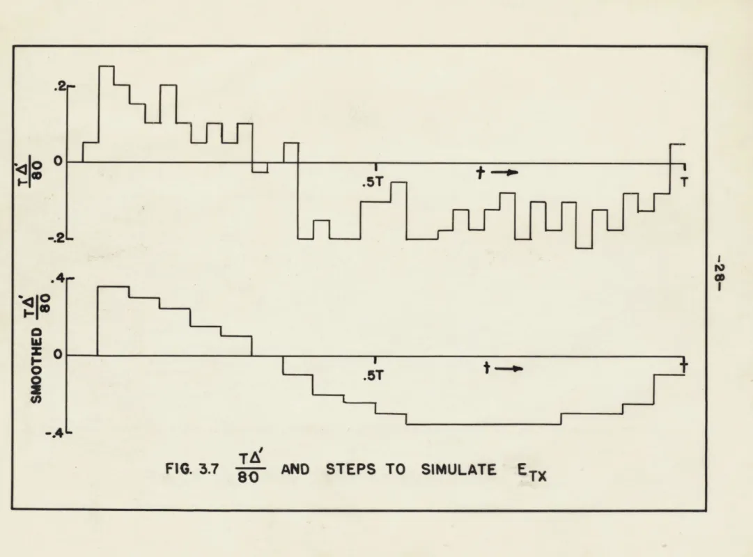
The plots of the first differences of X, Y, and 6 multiplied byr are

given in Figs. 3.7, 3.8, and 3.9. The second differences of * multiplied by T/b480 are given in Fig. 3.10.

Since a reduction in the amount of numerical work was desirable, the

following scheme was used to reduce the work. The smoothed truncation error curves were sampled at 0.05T-second intervals. The size of the samples was increased by a factor of two since the number of error steps (intervals at which a truncation error occurs) was decreased by two.

An examination of the truncation error in * reveqls that this error seems to be alternately positive and negative and as a result has very

.5T

.4-rI

0

.T.4E

I F

lnII

F

I

.5T

.5T

AND STEPS TO SIMULATE ETY

FIG. 3.8

80

.1

-E

e%

ro

₄₀ i

T

T

T

K m ...

-46--1

sy

.

LLJ

.5T

.5T

L~Lj

t

STEPS TO SIMULATE

80d

4o 0

Do.

nFlJ

.00or

7',

0a:I

x-'

T

0

05 L I

T

...

...

E:l

.0010-L--,--i

FIG. 3.9

AND

_{E TO}

m-

M

.

H-.ST

H1

'UI

t

-7

4TLF

IL

T

T

STEPS TO SIMULATE

.ir

II

nl

L

1_

-. ' ?..mmmm.~ w

0J

I

FIG.

3.10

Tb*AND

.a5

w

ET *

io 0

_wo

1--I*

little effect upon X. The truncation error in * is almost insignificant in comparison with the other errors when convolved with QX*. This is

evidenced by noting the scale used in the graphs relating these quantities. Although a crude approximation for E was made, the step response was such that the contribution to the total correction was negligible from this source of error. The major contribution to the correction arose from

truncation errors in 0 and X. An inspection of the magnitude of the step

responses and the magnitude of ETO and En shows that these two sources were the major contributors to the total correction curves.

3..4. Roundoff Errors.

The roundoff error cannot be handled as precisely as the truncation error since roundoff is a statistical variation and is not a function of the equations being handled. The probability of having a roundoff error can be handled. The maximum value caused by roundoff and a possible standard deviation of the error originating at each time interval will be attempted here.

The Newton-Gregory formula used ty. the computing section of the lab-oratory when written in terms of the ordinates rather than differences becomes

Z _n =Z _n-1 + hZ, _n

3.14

when neglecting the first differences, and

Z =Z _{n n-l} +Z"

Z

3.l<

2 n n-3

Z =Z +- Z

5 + 8 Z -Z3,16

when using first and second differences respectively. If the Z's are

assumed correct and the maximum roundoff error in the ZVs 'is e, the maximum contribution to the Z' s from the Z' s will be

= ch c 6 3.17

The factor I c

iwould

be equal to one when no differences or first

differences are used, but would be equal to 14/12 when second differences are used. Equation 3.17 shows that the maximum error in Z caused by a -roundoff of & in Z will be reduced by the interval of tabulation, h. The standard deviation of the error can be found by using the material in Appendix A.

The preceding discussion indicates that the contribution of roundoff

in Z to Z isnot significant. The contribution of an error in the solution is attributed mainly to the roundoff in the variable. The maximuim error in I would occur if a roundoff error of the same sign occurred in every variable for a period of time. The committed error function would be e in this case, if maximum roundoff errors are assumed. If the probabili-ty of having a roundoff error of magnitude O:Se :S is unifoigq, then the

probability of having an error e would be P(e )de and the standard deviation would be

a =2 e2P(e )de = e

03

The resultant error function would have a standard deviation equal toft/3. Since the errors have an equal chance of being either positive or negative,

the resultant error in X will be almost negligible, when the convolution with the step response is perfonmed.

Roundoff errors can be assumed random when the change in the quantity at each interval is greater than the maximum roundoff error. The only qiantity in the check solution that did not satisfy this criterion was the variable X. The change in XIwas less than the roundoff for a period of 8 intervals when X reached a maximum value somewhere between a - 0.5

and a - 0.7. With this exception the rest of the variables changed rapidly

enough, so that the effects of roundoff could be neglected.

3.5. The Resultant Correction.

The resultant correction was obtained by summing the result of the

convolutions of the approximation to the truncation error (roundoff errors

are neglected) and the respective step responses. For the second section

0.4S a SO. 8 the correction was obtained by using the terminal conditions

of the first section as well as the errors existing in the second section. The resultant correction is plotted in Fig. 3.11 as a dotted curve. The

solid curve is the approximation to the actual difference between the two check solutions determined by the computing section.

The apparent displacement in the solid curve after aT = 0.45T seconds

was caused by X reaching a maximum value and remaining at this maximum value for 0.15T seconds. The inclusion of this roundoff error in the calculated

correction would give a closer, but not exact, agreement between the two

curves.

The occurrence of this gross roundoff error cannot be predicted, but its effect is not serious since a cursory examination of Fig. 3.11 indicates that the cumulative error for the majority of the solution is in the order of magnitude of the roundoff error in I. Notice should be given also to

- ACT

---

CAL

TIME Of SECTIONING 0

O3T

0.4T

FIG. 3.11

ACTUAL

.5T

O.AT

.T

0

UAL

CULATED

0 0

cor

A

#

A'

/

A

AND CALCULATED

Cx

.IT

k

02T

7,

x

u

-1.5,

4S

.

0,!T

_I 05} C

..&-

.00-a- 1001A

the smoothing effect of integration on errors in (. The further that the errors are removed from the point of interest, the less the effect of the error. The more integrations that have to be performed before the effect is felt, the less is the effect.

The more sections used, the more accurate the resultant error to the actual propagated error. If the amount of sectioning is carried to its extreme, the result is the solution of the variation equations without

sectioning. A superficial examination of Fig. 3.11 indicates that the

resultant correction gives the order of magnitude of the error, but not the

exact form. These results indicate that a rough estimate of the error can be made from a very few sections.

The last section .8Sagl was not performed since the object of this chapter was to verify the validity of the sectioning and linearizing assumptions for this error analysis technique. For the purposes of error

study this complete survey need not be made since a set of step. responses

would give the desired information concerning the sensitivity of the various

sections to errors. Determination of the step responses is the beginning

to the error analysis study made by Rabow, in which the step responses were obtained by superimposing a step (error) upon a solution and recording

the variation that resulted from this step when compared to the original solution. The sAeps were inserted in the different variables and the results recorded at the various points of interest. The time at which

the steps were initiated was also varied. The proper interpretation of these step responses gave the weighting function that related the error committed and the propagated error at a later time.

The "H" matrix technique gives a method of obtaining these step responses during the presetup stage. The responses obtained are only approximations to the experimentally obtained responses. Although the pulses of error used in this chapter were the errors present in using a

numerical process, the errors could just as well have been errors in the

computer functional elements. A more efficient use of error analysis can

probably be made when the two techniques are combined; therefore, the

following chapter will show how a step response may be obtained at various

times during a solution by using the information obtained from the "H"

0036-.

Chapter IV

The study of the propagation of errors in analog computers by Jones3 used a weighting function which is the relationship between the error at various times during a solution and the error that has accumulated at a later time T in a solution. This weighting function can be obtained by properly analyzing a set of step responses for the particular system. This chapter illustrates the correlation between the step response obtained experimentally and the one calculated by the "H" matrix.

4.0. Adjoint Method.

The weighting function is the solution of the adjoint equations which are a set of equations in which the "H" matrix has been transposed'with a negative sign.

=

[H

ta _4.1

a] = H] .2

If Eq. 4.3 is premultiplied with Eq. 2.11 the result is

W.QWA~C [H].1[1 C =f CZ 4.4

or

+

JCZ

= 4 .5

but

Therefore

d CZ =

_4.7

and by integrating from time t to T

T d14CZ dt = 0 _4.8

c(T)CZ(T) + a2(T)CZ2 (T) *

- at)CZ1 (t,) a+ a2 (a )CZ2 t) + .. 9 = 0

1,9

If the boundary conditions of a n (T) 1 ., ap (T) 0 when p / n, the equation reduces to

CZ n (T) a nl(t )CZ ) + n2 a 2 a) + . . ..

An inspection of the final equations shows that the propagated error at time T is the weighted sum of the errors present at t in the variables. All errors must be changed to an equivalent error in one or more of the variables. The solutions of the adjoint equations may be rather difficult, but a system to obtain them experimentally was devised by Jones and verified by Rabow. The essence of this method was to purposely insert an error

(a step) at various times in a solution and to compare the results iith a solution that was run without the error (the step) inserted. The difference between the two solutions (with and without the error) was the step response to an error at the time when the step was initiated. The difference at a

time T in the two solutions was plotted against the time at which the error was inserted as the base. The resultant curves gave the weighting function.

4.1.

Pulse Response by Using "H" Matrix.

The step response at various points in a solution is obtained by the "H" matrix method. Since the problem is sectioned so that a constant "H" matrix can be assumed, the step response is the same regardless of when the error is inserted during a section of the problem. The responses are dif-ferent for difdif-ferent sections. The time response to an error originating

in a section is

CZ =V e '- t .V

For the purpose of illustrating how to obtain these step responses, a

hypo-thetical problem with two variables which has been sectioned into two parts

will be used. The point of sectioning is at time t s The response in the

two variables due to an error occurring at time t where 0 Ct is or

ts t a T,

CZ ~tta ₌ Ka t

cz.1

(ta) _{2 X}

2 _{1 (ta}

CZ2 1 = l + K 2Ke 2Y2 (t*

The propagated error in Z caused by errors present in both Z and Z2 at

-1 ) 2 2 a

CZ = L le _{+ L e Y (ta)}

Two types of step resonses can be obtained, one when the step is

inserted into the same variable that is being measured, and the other when the step is inserted into a different variable. If a step is inserted in

Z during the period t 4 t < T and the response in Z is desired, then

1 ~~s a CL a

Cz is the desired step response. The superscripts refer to the section of the solution. A step initiated at a time 0 Q t t in Z requires that

1 1

CZ and CZ for the first section be calculated until time t - t The

11 21 s a

step response during the first section is CZ 1 _{The remainder of the step}

11

response (during the second section) is obtained by calculating CZ where the initiating steps are equal to the teminal values of CZ1 and CZ1 _at

11 21

time t s This procedure is carried out for as many times as there are sec-tions in the solution. The above procedure is used to obtain the step response of an error in the same variable as the one being measured.

If the step is inserted in Z2 and the response in Z is desired, then for the interval t (t ST the desired response is CZ 2. If the step is initiated at C i t < t then for the interval ta Ct the desired step response_CL5

5

1 1 1

in CZ 2 during the first section. The value of CZ 2 and CZ at time

t = t -t is the magnitude of the step used at time t_s 5 _s12 to obtain CZ 2 + CZ2_U1 for the second section.

4.2. Experimental Results.

The two step responses given in Fig. 4.1 as a solid line were obtained by Rabow by inserting a pulse into the input of integrators x and 0, respec-tively. This pulse in the integrand is equivalent to a step in the output. The responses are for the variable x. A general block diagram for the simu-lator setup used to obtain these pulse responses are given in Fig. 4.2, which

- -- CALCULATED

--- EXPERIIENTAL

-

-QIT

O2T

0.3T

04T

05T

t

O.6T

O.7T OST

Q9T

1.

AND CALCULATED

STEP

3

2

1

-0

--

2

-3

3

2

01

-.3

L

000-0 000 0-

-okr

1

rlo

I

P

02T

OiT

O.4T

OST

O6T

O7T

0

T

LOT

4

-r

RESPONSES

)T

-43-B

E(DRIVINO

FUNCTIOO

POT

-U-RECORD

POINT

J

w

POT.

A~

t9~

FIG.4.2 SIMULATOR SETUP DIAGRAM SHOWING RECORDING

& = A cos 0 + B cos dt = A sin 0 + B sin dt - f(x, y, w,

e, e)

at

dt dw

W

=

f(e,

0, w)

The pulse widths used were 0.3 seconds and the pulse- height was of such a magnitude that both the x and 0 shafts were displaced by 0.00333 units. Inaamuch -as the pulse is not an impulse, the shaft displacement is not an ideal step, but a step with a ramp front. As a result the CX in Fig. 4.2 did not start from 0.0033 but started from zero. The delay in the rise of CX was also due to the fact that a pulse was used rather

than a step.

The dotted line gives the same responses for an ideal step in using the initial conditions to the original differential equations in obtaining the "H" matrix. The equations for the step responses are

CX = 3.559 x 10-5 e-525.4aT - 3.394 x 10- 2 e-134.2aT

x

+ e-10.2aT 1.034 cos 20.17aT + ."'735 sin 20.17aT

CX₀ O -.068 e525.haT - 26.260 e-134.2aT

+ e-10.2aT [26.323 cos20.17aT - 1210 sin 20.17aTJ

The assumption of a constant "H" matrix cannot be made for an entire solution for the type of equations solved on the M.I.T. Flight Simulator.

A possible time of sectioning would be at a time of two thirds the

solution time. This would give closer agreement at the end of the responses. This step response without sectioning gives an indication of what can be expected by using only the initial values of the variables in solving the

H" matrix.

The conclusions to be drawn here are that the "H" matrix method can give the step responses necessary for obtaining the weighting functions by using a very few sections. The experimentally obtained step response is an approximation to the step response in that a pulse rather than an impulse is used in the integrator inputs. The precision of the simulator dictates the lower limit for the size of the pulse to be used, and the upper limit is reached when the error cannot be assumed to be an increment additive to the solution. The weighting function obtained by using pulse responses obtained by the "H" matrix can be made to correspond closely to experimental results if the solution is sectioned into possibly three sections.

Chapter V SOURCES OF ERBOR

The truncation and roundoff errors present at each numerical. tabulation are inherently associated with the integration formula used in the numerical process. The numerical technique used in the numerical computation (iterative

or extrapolation) has a marked effect on these errors. The propagation of these errors has been explained in the previous sections of this thesis, but the actual source of these errors has not been discussed. This section will elaborate on these errors.

5.0. Roundoff Errors.

The process of numerical computation involves the use of present and past information to obtain present or future information. The process can be integration, differentiation, extrapolation or any other mathematical operation. *he probability of having a roundoff in the result is dependent upon the coefficients multiplying the past information and the probabillity of roundoff in the past data. The maximum roundoff error will occur when the algebraic sum of the coefficients and the roundoff in the past ordinates or differences are a maximum. An indication of the magnitude of the maximum roundoff error that can occur is the sum of the absolute values of the

coefficients multiplied by the roundoff. The probability of having a roundoff error in a sum of numbers is dependent upon the coefficients mul-tiplying the numbers as explained in Appendix B. The roundoff error com-mitted at any step can be assumed random if the variable changes more than

the roundoff errors committed at each interval are comparable regardless of whether iteration or extrapolation techniques are used, the buildup of the error can become prohibitive in an extrapolation process. This buildup of the error will be explained in section 5.3.

5.l. Truncation Errors.

The magnitude of the truncation error is an indication of the accuracy of the numerical mathematical process of the variable to the true mathe-matical process. In the case of integration when a Newtonian integration

formula is used the truncation error committed is apprximately equal to the first neglected term in the formula, but if an infinite number of

terms are used then the process is exactly equivalent to a true integration. The more rapidly -the function to be integrated varies, the more "terms of the formula must be used to reduce the truncation error. The errors com-mitted in the various Newton formulas when the first, second, or third

differences are neglected are discussed in Chapter 3. This time domain approximation to the error committed gives an indication of the error com-mitted, but the signal frequency spectrum that the formula can handle is best expressed in the frequency domain. In the analog computation field,

the use of transfer functions .is prevalent and the numerical analysbt may find it useful to look at the numerical processes in the frequency domain. The closeness of the various integration formulas to 1/s when expressed in the frequency domain is an indication of the adequacy of the formula to the functions being integrated.

The Newton Gregory formula with no differences reduces to the simp3e integration formula

4n M 6n-i + n

5.1

which in the frequency domain becomes7

___ T

O(s) 1 - e-sT

When one difference is used the integration formula reduces to the trapezoidal rule

T 0

50

en n-1 + Sn n-1) .

and when two differences are used the integration formula becomes

() MT (5 + 8

n 6 n-1 + n + n-1 n-2)

The corresponding transfer functions for these integration formulas become

.906 , T + e-sT 2 -sT and T_ 5 + 8e's - e -2sT B(s) 12 -sT 5 respectively.

Each of the above integration formulas should reduce to 1/s in the range s = -A2 and s = * 2 where At= 21T/T if true integration is to be performed. By expanding e-sT into a series, Eqs. 5.2, 5.5, and 5.6 can be reduced to the following when sT is made small enough so that the

-4 T _{_} e-sT 1 - e-T T 1 + esT T 2 ~-sT 2T 1 - -2s T 5 + 8e~T -e2sT T2_ 1 - e-sT T sT(1 sT + 2 sTl 21 31. 2sT + (sT)2 ST +2. * sT (sT) T 12 - 6sT + 2L J2sT * sT (sT)2 1 2- + N + .1

Equations 5.7, 5.8, and 5.9 will approximate 1/s as follows.

T 1 e-sT s 1 sT (sT) 7- + -141 +. 5.10 5.11 sT +(sT)2

(sT)3

T 1 + e- 1 2 (2)(2') (2)(3+ 2 _{-s T s sT (} + T)3' 1 e1 + 3L._2 + T s + 8es-T _ e-2sT T s 1 - e-s' sT ~2 4 1 - + + (sT)4 - . . . = ~ 2 ~ 31 SsT (sT) (sT)3 3- + .L

The results indicate that Eq. 5.9 gives the smallest error, Eq. 5.8 the next smallest and Eq. 5.7 the largest error. These results are con-sistent with the results from the time domain analysis. For a fixed maximum frequency signal Eq. 5.7 can have the same accuracy as Eq. 5.9

if the interval of tabulation T for Eq. 5.7 is decreased by a sufficient amount. When the numerical integration formulas are expressed in the

frequency domain, the ability to handle a certain signal frequency spec-trm with a specified accuracy becomes evident.

5.2. Extrapolation.

Numerical analysts use two basic methods of approach to obtain a numerical solution to the type of equations solved on the M.I.T. Flight Simulator, The two methods are the iteration and extrapolation methods. 1_{n the iteration technique, the equations are cambined and arranged so} that if a value for one variable is assumed, then all other variables can be obtained by numerical integration or other mathematical relationships. AIfter the value for the first variable is chosen and the values for all the

other variables have been computed, one iteration is comple ted when the newly obtained variables are replaced in the original equations to determine

if a proper choioe for the assumed quantity was made. If the two values

(the assumed values and the values obtained by the numerical computations)

do not agree within the limits of accuracy specified, then another itera-tion is performed. Not until an agreement within the tolerances specified is reached does the computer advance to the next interval. This process, which can be likened to a servo system, can use a crude integration formula,

since the feedback loop (the original equations) is the most accurate meas-uring device that is available. The buildup of the errors cannot be great since each integrated value is substituted into the original equations for verification at each interval.

In the extrapolation method the values of the variable at previous intervals are weighted to obtain the value of the variable at the present interval. A relatively high accuracy formula. which is not susceptible to roundoff errors must be used since no verification is performed at each interval. An error can be made at one interval and will not be cor-rected as in the iterative.processes.

The buildup of errors has usually limited the number of consecutive steps that can be handled by extrapolation techniques. Wong has shown

that .the choice of extrapolation formulaa, so that the buildup of errors will at most be linear, must have the absolute magnitude of the largest coefficient multiplying the various past information around unity. As an illustration the following simultaneous linear differential equations were solvedi

* = x - y - 1 + 2t

S 2x - y + 3t + 1 5.13

x(O) - 1, y(O) = 0 using the extrapolation formula below:

Xn = n-4 + X-3 _{X n- +TX n-3 +}

TXn-. . 5.14

Y - Y + Y -Y +TY + TY

n n-4 n-3 n-l n-3 n.1

After the solution of the equations had been calculated for a number of intervals, the same intervals were recalculated with an error inserted at one interval in x. The difference of the two solutions was the step remponse to an error. This response shown in Fig. 5.l exhibits an unusual pattern, which was not expected from the analysis made by using the "H"

"Hv MATRIX

L~~J

___

I

211V4?Th-LL

FIG.

5.1

STEP RESPONSE

Li

-- ACT UAL

-4H" MATRIX

FOR AN EXTRAPOLATION PROCESS

.00m 0 'C 0 ACTUAL

.0008

.0005

K

>~ 0 0 I

ro

_a

.0005

U I i i I 1 1 1

H = $.15

2

-The characteristic roots of the "IIH matrix are tjl. The equations for the step response using characteristic and dual vectors as explained

in chapter IIbecome CX 1 1 e 0 -a. 1 2j 2j x 5.16 CY 1-j 1+j 0 e-jt 1 J L J L2j 2j y or Cy - -sin t 5.17 CX _x - 2 sin (t + 45*)

The answer to the pattern was that an error in one variable was not inserted once, but four times by the extrapolation formula. Ah examination of the extrapolation formula in Eqs. 5.14 reveals that if an error was committed in one interval, then the pattern of the errors in succeeding intervals

would be as follows: 1, -1, 1, 0, 0, 0, 1, -1, 1, 0, 0, 0, The pattern repeats itself after 6 intervals. The effect of the errors in

the derivatives was neglected since these errors mem diminished by the interval of tabulation (.03). The actual error in x would be the running

sum of the errors committed' at each step, therefore the extrapolation

for-mula used has a linear buildup of errors. The smoothing effect due to decreasing the interval of tabulation which occurs in an iteration process was not present in the extrapolation technique. In fact the more steps required for a solution the more likely the accumulation of a large error when using an extrapolation technique.

The iteration process may require considerable time when a slow-speed computing machine is used and a large amount of iteration is required at each step. On the other hand the buildup of errors when using an extrapo-lation technique may render a computation useless if a large number of steps are required in the solution. A compromise between the two would be to use iteration, for example, at every tenth step and extrapolation at other times. A watch on the differences would indicate when a computation

is becoming useless due to the inadequacy of the numerical process. The

type of equations solved on the M.I.T. Flight Simulator is such that the

Chapter VI

SUMMARY AND CONCLUSIONS

A correction can be found to compensate for the errors committed at each interval of tabulation. The errors present at each interval must be known to obtain the actual correction, but for error analysis purposes the obtaining of the step response is sufficient. These sensitivity functions indicate the susceptibility of the solution of the differential equations to an error in any of the variables. This scheme is not a catholicon for errors in a numerical solution, but is rather a method of assessing the adequacy of the solution for the purposes of checking the M.I.T. Flight

Simulator.

6.0. Location of Characteristic Values on Complex Plane.

The behavior of the errors can be obtained by a cursory examination

of the location of the roots of the characteristic equations in the complex plane. A root in the left half plane indicates that the errors will die out, whereas a root in the right half plane indicates that the errors will increase with time. The root locations change with time as well as with parametric changes of the differential equations. The movement of the root locations is towards the right half plane as the problem progresses for the type of equations simulated on the M.I.T. Flight Simulator.

Although errors committed near the end of the solution do not die out, the buildup in the remaining time can not become excessive and the solution is still valid at the end.