Design and analysis of jammable granular systems

Design and Analysis of Jammable Granular Systems by

Nadia G. Cheng

B.S. Aerospace Engineering, University of California, San Diego, 2007 S.M. Mechanical Engineering, Massachusetts Institute of Technology, 2009

Submitted to the Department of Mechanical Engineering in Partial Fulfillment of the Requirements for the Degree of

Doctor of Philosophy at the

Massachusetts Institute of Technology June 2013

ARCHIVES

@ 2013 Massachusetts Institute of Technology. All rights reserved.

Signature of A uth or...,... . . . . ... ... ... Department of Mechanical Ji 'ineering

a 10, 2013

C e rtifie d b y ...

Karl Iagnemma Principal Research Scientist of Mechanical Engineering Thesis Supervisor

C e rtifie d b y ... - ... ... Anette Hosoi Associate Professor of Mechanical Engineering Thesis Supervisor

A ccep te d b y ... K 7..'...

Design and Analysis of Jammable Granular Systems by

Nadia G. Cheng

Submitted to the Department of Mechanical Engineering on May 10, 2013 in Partial Fulfillment of the Requirements for the Degree of Doctor of Philosophy in

Mechanical Engineering

ABSTRACT

Jamming-the mechanism by which granular media can transition between liquid-like and solid-like states-has recently been demonstrated as a variable strength and stiffness mechanism in a range of applications. As a low-cost and simple means for achieving tunable mechanical properties, jamming has been used in systems ranging from architectural to medical ones. This thesis explores the utility of jamming for robotic manipulation applications, both at a fundamental level of understanding how granular properties affect the performance of jammed systems, and at a more applied level of designing functional robotic components.

Specifically, the purpose of this thesis was to enable engineers to design jammable robotic systems in a principled manner. Three parallel yet related studies were conducted to work towards this goal. First, an experimental analysis was conducted to determine whether the bulk shear strength of granular systems can be correlated with grain properties-such as ones concerning shape, size distribution, and surface texture-extracted from 2D silhouettes of grains. Second, a novel medium composed of a mixture of hard and soft spheres was proposed to achieve variable strength and stiffness properties as a function of confining pressure; experimental analysis was conducted on this system with not only varying confining pressures but also varying mixing ratios of hard and soft spheres. Finally, the design and analysis of a novel jammable robotic manipulator-with the goal of maximizing both the strength and articulation of the system-is presented. Thesis Supervisors: Karl lagnemmal and Anette (Peko) Hosoi2

Title: 'Principal Research Scientist and 2Associate Professor of Mechanical Engineering

ACKNOWLEDGEMENTS

First and foremost, I thank my thesis advisors Dr. Karl Iagnemma and Prof. Anette (Peko) Hosoi. Their constant support, encouragement, and enthusiasm have enabled me to steadily learn and mature as a researcher and engineer. It has been an absolute honor to be mentored by them. I also extend my gratitude to the other members of my thesis committee, Prof. Sangbae Kim and Dr. John (Jack) Germaine; their wisdom and thoughtful advice have not only contributed to the quality of my work but also to my growth as a researcher.

Much of the knowledge and lifelong friendships I developed have been through the collaborative research project I was part of (funded by the DARPA Chemical Robots and M3 programs) throughout my entire time at MIT. Thank you to, in addition to my advisors, Prof. Gareth McKinley, Prof. Martin Culpepper, Dr. Arvind Gopinath, Dr. Bian Qian, the folks at Boston Dynamics, (now Prof.) Randy Ewoldt, Sarah Bates, Maria Telleria, Jeff Morin, Ahmed Helal, and Nick Wiltsie. I could not have asked for a more supportive and fun group of people to work towards challenging deadlines with.

I am also very grateful to all the UROPs I have worked with: Katy Gero, Hao Chen, Stephan Hawthorne, Alexis Hakimi, Sara Falcone, Shaymus Hudson, and Jorge Perez. I greatly appreciate all their patience and trust in me, and I hope that they have benefited as much as I have from our time working together. I am also extremely thankful to those who have selflessly taken the time to help me in my work: Steven Keating, Mark Belanger, Amy Adams, Stephen Rudolph, Dr. Germaine, Robin Deits, and Max Lobovsky.

I also thank all the students and postdocs who have been part of the Robotic Mobility Group, Team Peko, as well as the Laboratory for Manufacturing and Productivity and the Hatsopoulos Microfluids Laboratory. I have been so lucky to learn from and be surrounded by such talented and kind individuals every day.

I have also been very fortunate to have the opportunity to work on exciting and challenging side projects that have made my time at MIT all the more fruitful. Many thanks

Jason Spingarn-Koff, Ostap Rudakevych, Natan Linder, Sean Follmer, Daniel Leithinger, and Alex Olwal.

I am forever grateful to my talented and inspiring teachers and mentors from various stages and aspects of my life: Diana Ng Cheng, Dr. Victor Cheng, Prof. Claire Tomlin, Dr. P. K. Menon, Dr. Banavar Sridhar, Dr. Shon Grabbe, Prof. Keiko Nomura, Dr. Evelyne Kolb, Mrs. Paula Spaulding, Zoe Austin, Carlos Carvajal, Christine Leslie, and Robin Offley-Thompson. Their patience and faith in me have given me courage to keep challenging myself with the knowledge that even if I come up short, I am bettering myself.

Thank you to my college colleagues and dear friends-Greg Nichols,

Jean-Paul

Many, many thanks to Ahmed Helal, Maria Telleria, and Lisa Burton for not only being wonderful colleagues but also some of my dearest friends. I know that I have been very fortunate to be around such selfless individuals who inspire those around them to be better people.

Thank you to Max, my partner and best friend.

And last but not least, I thank my family, especially my sister, Lara, and my parents, whose sheer love and belief in me have propelled me further than I ever would have thought possible at every step of my life.

Dedicated to my parents, whose love and teachings in the value of hard work have given me the most blessed life.

CONTENTS

A bstract ... 3

A cknow ledgem ents ... 5

Contents...8

Figures...11

Tables ... 16

1 Introduction ... 17

1.1 M otivation and overview ... 17

1.1.1 Research goals... 18

1.2 Soft robotics: background... 20

1.2.1 Tunable strength and stiffness mechanisms ... 21

1.3 Jam m ing of granular m edia: background ... 22

1.3.1 Physics... 23

1.3.2 Soil m echanics ... 23

1.3.3

Jam

2 Relating granular properties to bulk performance ... 26

2.1 Background and m otivation ... 26

2.1.1 Characterizing "microscopic" grain properties: background ... 28

2.2 Friction angle... 29

2.3 Experim ental m ethods and procedure... 30

2.3.1 Grain selection... 30

2.3.2 Im aging analysis ... 30

2.3.3 D irect shear tests... 34

2.3.4 Triaxial tests... 37

2.3.5 D irect shear vs. triaxial tests... 39

2.4.1 Circularity and polydispersivity vs. friction angle ... 40

2.4.2 Density vs. friction angle ... 42

2.4.3 Surface properties... 44

2.5 Conclusions ... 45

2.6 Recom mended next steps... 46

3 Exploration of stress-dependent properties in granular systems ... 47

3.1 Background and motivation ... 47

3.1.1 Rubber-sand mixtures in soil mechanics studies ... 49

3.2 Experimental methods and procedure... 50

3.2.1 Determining -3 for the case of no applied vacuum pressure ... 52

3.3 Results and Discussion ... 53

3.3.1 Bulk compression modulus and yield stress ... 53

3.3.2 Bulk compression modulus, effective friction angle, and percolation... 57

3.3.3 Effective friction angle and angle of repose... 59

3.3.4 Predictive models for the bulk compression modulus ... 61

3.4 Conclusions ... 67

3.4.1 Recom mended next steps... 67

4 Design and analysis of a jammable robotic manipulator ... 69

4 .1 O v erv iew ... 6 9 4.2 Hyper-redundant robotics: background... 70

4.3 Strength-to-weight performance... 71

4.3.1 Experimental methods and procedure ... 71

4.3.2 Experimental results and discussion... 73

4.4 Design of jammable manipulator prototypes ... 75

4.4.1 Overview ... 75

4.4.2 Prototype 1... 76

4.4.3 Prototype 2... 77

4.4.3.1 Design of jammable segments ... 77

4.5.1 Speed... 79

4.5.2 Strength...80

4.5.3 Dexterity and articulation w ith sim ple control... 82

4.6 Predicting the bending strength of a jam m able beam ... 84

4.6.1 Com paring theory w ith experim ental results... 85

4.7 Conclusions ... 87

4.8 Recom m ended next steps... 87

4.8.1 M anipulator design... 87

4.8.2 Feedback and control ... 88

4.8.3 Potential applications... 88

5 Conclusions ... 90

A Derivation for predicting the maximum bending moment of a jammable beam ... 93

A.1 M odeling a "jam m able" beam as a com posite beam ... 93

A.1.1 Empirically determining parameters for compressive and tensile jammable elem ents... 98

FIGURES

Figure 1.1: A schematic of a jammable system composed of granular media contained in an elastic, impermeable membrane. The differential jamming pressure, Pjam, can be controlled by a vacuum pump, and is defined as Pjam = Pout - Pin where Pout is the ambient pressure outside of the system and Pin, is the pressure inside the system. (Diagram s: courtesy of Steven Keating.)... 18 Figure 1.2: A visual representation of where the three studies presented in this thesis might

fall along a spectrum of "jamming" research, which encompasses fundamental physics, soil mechanics, and jamming applications... 19 Figure 1.3: A sampling of jamming applications across various fields. Applications include: a universal gripper [2][49]; a soft, mobile robot [50][51]; tangible user interfaces [7]; an endoscopic tube [4]; architectural structures [5][6]; and reconfigurable molding and casting devices (Steven Keating, M IT). ... 25 Figure 2.1: A visual representation of the goal of the work presented in this chapter, which is to correlate "microscopic" properties of individual grains with the "macroscopic" perform ance of the bulk system ... 28 Figure 2.2: Example of raw and binary images of grains. ... 31 Figure 2.3: The running average for the parameter "aspect ratio" vs. the number of particles considered for kosher salt grains; each of the five curves represents a unique distribution of grains in a single photograph... 34 Figure 2.4: A schematic of the direct shear test set-up ... 35 Figure 2.5: An example of results from direct shear tests for ground coffee. The inset graph presents the shear stress vs. displacement data for three different applied normal loads. The main graph presents the maximum shear stress versus the applied normal load. This latter curve is expected to be linear, and its angle relative to the horizontal axis is defined as the friction angle, a, of the material. Note that a non-zero vertical intercept in the main plot indicates that the material exhibits cohesion (i.e., the curve

Figure 2.6: A schematic of the triaxial test set-up used to determine the friction angle, a, of a set of grains, which were contained in a cylindrical, thin elastic membrane sealed off by two rigid end plates. Labeled parameters: isotropic confining pressure U₃, which is

the vacuum pressure (Uvac) applied to the inside of the cell; and a1, which is equal to the sum of the axial yield stress (ay) and the confining vacuum pressure. or and U3 are the principal stresses in the system and are used to calculate the friction angle.. 37 Figure 2.7: A schematic describing how the Mohr-Coulomb failure criterion is used to

determine the friction angle, a, of a set of cohesionless grains. Note that a is expected to remain constant for a limited range of u3 values (or confining pressures)... 38

Figure 2.8: A comparison of friction angle, a, as determined from triaxial compression tests vs. direct shear tests. The dotted line with a slope of one serves as a visual aide to compare how a differs between the two types of experiments (if the results between the two experiments were identical then all the points would lie on this line)... 39 Figure 2.9: Friction angle, a, vs. the inverse of circularity, C-1... 41 Figure 2.10: Friction angle, a, vs. polydispersivity, P... 42 Figure 2.11: Friction angle, a, vs. the bulk density of different granular systems: 1) sand, 2) 390 jim glass beads, 3) Folgers ground coffee, 4) diatomaceous earth, 5) cumin seeds, 6) Jasmine rice, 7) couscous, 8) sesame seeds (unhulled), 9) amaranth grain, 10) oat bran, 11) corn grit, 12) poppy seeds, 13) table salt, 14) kosher salt, 15) sesame seeds (hulled), 16) quinoa, 17) sandblasting glass beads, 18) Goya rice, 19) 300-425 jIm glass beads, 20) 800-1200 [tm glass beads, 21) 1500-2000 [tm glass beads, 2) 2000-2500 jm glass beads, 23) finely ground coffee, 24) medium-ground coffee, 25) coarsely ground coffee... 4 3 Figure 2.12: SEM images of two types of sesame seeds tested: a) hulled and b) unhulled.. 45 Figure 3.1: A photo of grains from the outside of a triaxial cell during a test; the scale bar rep resen ts 5 m m ... 4 9 Figure 3.2: Effective modulus, Eff, vs. compressive yield stress, cy. Solid lines connect points for a given volume fraction of soft spheres, T, (values labeled at the rightmost end of each curve), while dotted lines connect points for a given confining pressure, -3 (designated by different marker shapes and corresponding values in the legend)...55

Figure 3.3: Effective modulus, Eeff, vs. compressive yield stress, U3 for the cases of V, = 0 and V, = 1. The lines represent power law fits for each case: the dotted lines represent fits including all four data points in each case, while the solid lines represent fits that include only three data points for q3 34 kPa in each case...57

Figure 3.4: Effective compression modulus, Eeff, and effective friction angle, aeff, vs. V, for various values of q3. The red and blue shaded regions reflect the overall trends of

Eeff and aeff, respectively, for q3 34 kPa. The shaded vertical bars at

approximately V, = 0.29 and V, = 0.71 indicate the theoretical percolation thresholds for the soft and hard spheres, respectively ... 59 Figure 3.5: Effective friction angle, ae/f, vs. Vs for various values of a3. The solid circle and

square markers represent the angle of repose for the case of "no rolling" and "rolling", respectively. In the case of "no rolling", the bottom layer of the grains was contained in a circular dish such that they were not allowed to roll laterally; in the case of "rolling", the grains were placed on a large horizontal surface such that the bottom layer of grains was allowed to roll and move laterally... 61 Figure 3.6: A diagram of the idealized system used to calculate a theoretical value of the

bulk compressive stiffness, Eeff using a Monte Carlo simulation. Each square (or unit) represents a sphere in the real system. Note that the ratio of units labeled Eh to those labeled Es depends on the value of Vs, which is specified by the user in the

sim u latio n ... 6 4 Figure 3.7: Normalized bulk modulus, Eeff, vs. volume fraction of soft spheres, Vs, where the Eeff = Eeff Ee*f and E* is the effective compressive modulus when Vs = 1.

Both a closed-form and three numerical solutions are included. The solution calculated from the Bache and Nepper-Christensen model (labeled "BNC model") is also included for com parison [82]... 66 Figure 4.1: Two prototypes of the jammable robotic manipulator: a) the first prototype, and (b) the second prototype: (left) in the unjammed state, and (right) jammed in a corkscrew configuration... 70

Figure 4.2: Microscope images of the grains tested. Top row, left to right: coarsely ground coffee, finely ground coffee, sawdust; bottom row, left to right: solid glass spheres, hollow glass spheres, and diatom aceous earth ... 72 Figure 4.3: Compressive stress vs. strain data for the grains tested... 73 Figure 4.4: A schematic illustrating how serially connected tunable stiffness elements can be coupled with simple external actuation to achieve complex and arbitrary co n figu ratio n s... 7 6 Figure 4.5: A CAD drawing showing a cross-sectional view of the second prototype of the manipulator; schematics of primary system components are also included and lab e le d ... 7 8 Figure 4.6: Tip load vs. displacement curves for the cantilevered, jammed manipulator. One test was conducted with activated tension cables along the top of the manipulator to provide tensile strength; the other test was conducted without the use of tension cables. The dotted line represents the linear fit for the apparent elastic regime for the fo rm er case...8 1 Figure 4.7: A comparison of various manipulator technologies: the Octopus Project [12], the OctArm [16], a surgical robot [89], a personal robot [92], the Festo bionic handling assistant [17], a search-and-rescue robot [93], and an elephant trunk composed of springs and cables [88]. The parameters of interest were the flexibility of the robot (quantified as length/radius of curvature) and relative payload capacity (quantified as maximum transverse payload/manipulator mass)... 82 Figure 4.8: The manipulator demonstrating its ability to: a) reach an end effector target with multiple configurations, and b) achieve many complex and highly articulated shapes. Note that the manipulator is jammed to rigidly hold its shape in all these im a g e s... 8 3 Figure 4.9: A series of images (sequentially labeled) extracted from a video that demonstrated the manipulator operating in a confined environment with obstacles to achieve a desired end-effector position (indicated with the left-most, black peg)...84

Figure 4.10: The theoretical maximum bending moment, Mmax, vs. the effective bulk tensile modulus of ground coffee, Et. The empirical values used in (4.1) to calculate Mmax were determined for the case of Pi am = 101 kPa... 86 Figure A.1: A series of diagrams illustrating the parameters used in (A.1)-(A.8) for a

rectangular cross section of a beam composed to a tensile element with

cross-sectional area A1 and a compressive element with cross-sectional area A2. . . . ...----... . 96

Figure A.2: A diagram illustrating the parameters used in (A.9)-(A.12) for a circular beam cross section composed of a tensile element with cross-sectional area A1 and a

compressive element with cross-sectional area A2 .---. . . .. --- . 97

Figure A.3: The normalized distance, d, (of the neutral axis from the center of the beam for the case of a rectangular and circular cross section) vs. E2E... 97 Figure A.4: Engineering stress vs. engineering strain data from the triaxial compression tests conducted on coarsely ground coffee. Different-colored curves represent tests conducted at various differential jamming pressures, Pam, as specified in the legend. ... 9 9 Figure A.5: Engineering stress vs. engineering strain data from the triaxial tensile tests conducted on coarsely ground coffee. Different-colored curves represent tests conducted at various differential jamming pressures, Pam, as specified in the legend. ... 1 0 0

TABLES

Table 1.1: A comparison of various phase-change and "smart" materials that are capable of transitioning between a solid (or solid-like) state and a liquid (or liquid-like state). 22 Table 2.1: An example of grain parameters extracted from ImageJ for a batch of ground coffee photographed five times, each time after randomly redistributing the grains on a flat, horizontal surface... 33 Table 4.1: Empirical values for stiffness-to-density, Eeff/p, yield stress, ay, and strength-to-density, 0y/p, for the m aterials tested... 74 Table A.1: Effective modulus and yield stress values extracted from the data presented in

Figure A.4 and Figure A.5, where Ec is the compressive modulus, and Uyc and -y't were the compressive and tensile yield stresses, respectively...100

CHAPTER

1

INTRODUCTION

1.1 Motivation and overview

The motivation for this thesis was to contribute to the field of soft robotics by furthering the understanding of "jamming" of granular media as a means for achieving variable strength and stiffness components. Jamming is the mechanism by which granular media can reversibly transition between fluid-like and solid-like states [1], and while physicists have studied the intricacies of the jamming phenomenon for decades, designers and engineers have only recently adopted it as a simple mechanism for achieving tunable strength and stiffness components in many applications. The breadth of jamming applications introduced in the last several years includes robotic end effectors [2] and manipulators [3], medical devices [4], reconfigurable architectural structures [5][6], and haptic and tangible user interfaces [7][8].

Such systems demonstrate the relevance of jamming in real-world applications because they can be cheaply and readily realizable and capable of rapidly transitioning between relatively large ranges of strengths and stiffnesses. In most of these systems-which we will refer to as "jamming applications"-the bulk behavior of the system is

controlled by specifying the confining pressure acting on the system, which is often composed of grains contained in an impermeable and elastic membrane. Therefore, a simple component such as a vacuum pump can be used to modulate the differential jamming pressure, Pam, of the system [2], as illustrated in Figure 1.1.

un-jammed state

jammed state

"fluid"

"solid"

elastomer _{interstitial fluid} bladder _{() (often air)}

PP

O

Pout

6Q

0

0

granular

O

media _pump

atmospheric pressure

Figure 1.1: A schematic of a jammable system composed of granular media contained in an elastic, impermeable membrane. The differential jamming pressure, Pjam, can be controlled by a vacuum pump, and is defined as Pjam = Pout - Pin, where Pout is the ambient pressure

outside of the system and Pin is the pressure inside the system. (Diagrams: courtesy of Steven Keating.)

The combination of the aforementioned projects highlights the primary benefits of utilizing jamming for robotics: it enables robots to be more human-safe, inexpensive, and robust compared to most technologies that have traditionally been used for such applications.

1.1.1 Research goals

The overarching goal of this research was to enable engineers to design jammable robotic systems in a principled manner. Within this scope, several areas were highlighted:

1. evaluating the strength and stiffness of granular systems in the context of jammable applications;

2. correlating granular properties with the bulk performance of systems; and 3. robotic manipulation applications.

This thesis presents an exploration of these areas through three parallel yet related studies, each of which is discussed thoroughly in Chapters 2-4:

1. Chapter 2 presents an experimental analysis of whether the bulk shear strength of granular systems can be correlated with grain properties extracted from 2D silhouettes of individual grains;

2. Chapter 3 introduces a novel granular medium-specifically, a mixture of hard and soft spheres-and an experimental analysis of whether it can achieve tunable strength and stiffness properties as a function of mixing ratio and confining pressure; and

3. Chapter 4 presents the design and analysis of a novel, jammable robotic manipulator.

Figure 1.2 presents a visual representation of where these studies might fall along a spectrum that broadly encompasses disciplines-namely, physics, soil mechanics, and jamming applications-that contribute to the study and application of jamming. Section

1.3 presents a brief background of each of these disciplines in the context of jamming.

fundamental physics soil mechanics jamming applications

micro ++ macro novel tunable jammable robotic

grain properties granular systems manipulator

1

Figure 1.2: A visual representation of where the three studies presented in this thesis might fall along a spectrum of "jamming" research, which encompasses fundamental

1.2 Soft robotics: background

While the term "soft robotics" is not yet well defined, it is apparent why researchers are interested in making robots softer: traditional systems often utilize distributed, rigid components such as electric motors, which might limit a robot's range of motion and abilities to conform to complex environments. More importantly, in comparison to a system such as an elephant's trunk, which is composed of continuous structures that are flexible and can be "actuated," traditional robotic systems can be relatively fragile and therefore lack robustness. However, the benefits of traditional robotic components-including high force output, bandwidth, and repeatability-are often what existing "soft robots" lack due to the dearth of technologies that are both physically compliant and have high mechanical performance output.

There have been many approaches to making robots softer by replacing traditional actuators with more compliant ones enabled by technologies such as shape memory alloy and polymer actuators [9]. Though impressive and physically compliant, many of these technologies are not ideal for robotic applications because they are incapable of large force outputs and high-bandwidth operations. For example, as part of a thrust to design a system that mimics an octopus tentacle, a robotic arm composed of a silicone body and shape memory alloy actuators was developed; though highly articulated, this arm lacked the bending strength and stiffness required for many manipulator applications [10][11][12]. Additional examples of compliant yet low-force systems that have contributed to the field of soft robotics include a caterpillar-inspired robot [13] and an extremely lightweight mobile robot composed of a Nitinol mesh [14][15].

Another approach to realizing soft robotics is through hydrostatics; for example, portions of a robot can be composed of bladders that can both change shape and apply forces on the environment by controlling the fluid pressure in the system [16][17][18]. The benefits of this type of system include: the effective stiffness of the bladder can be tuned based on the supplied fluid pressure, and force outputs can be relatively high depending on the fluid pressure. Because small (mm- and cm-scale) traditional valves can be very expensive, researchers have also been developing novel valve technologies that enable components to be more discrete for these hydrostatic robotic systems [19] [20] [21].

However, in comparison to the jammable robotic manipulator presented in Chapter 4, hydrostatic robots cannot easily be controlled to embody arbitrary configurations because hydrostatic pressure would cause a bladder to expand to its natural inflated shape rather than maintain an arbitrary one.

A more thorough review of approaches to developing "soft" robotic manipulators is presented in Section 4.2.

1.2.1

Tunable strength and stiffness mechanisms

There are various phase-change and "smart" materials that are capable of transitioning between solid (or solid-like) and liquid (or liquid-like) states. Such materials would benefit soft robotic applications because they would enable systems to transition between rigid, load-bearing states and passively deformable ones.

For example, magnetorheological (MR) and electrorheological (ER) fluids-which consist of small metal particles (with dimensions on the order of tens of micrometers) suspended in a liquid-can exhibit yield stresses (and therefore behave like a solid) when a magnetic or electric field is applied, respectively. MR fluids have been proven to be very effective as rapidly tunable suspension and damping mechanisms in automotive and robotic applications [22][23][24][25]. MR fluid has even been proposed as a variable stiffness material for robotic gripping mechanisms [26]. However, even though MR and ER fluids can exhibit large impact strengths at high strain rates, their properties are highly strain-rate-dependent, yielding relatively low strengths and stiffnesses under quasi-static conditions.

Phase-change materials, including thermally tunable materials such as wax and solder, have also been proposed as variable stiffness mechanisms for soft robotic applications [27][28][29]. However, for thermally controllable materials, the significant amount of time and energy required to transition between states can be unreasonable for many robotic applications.

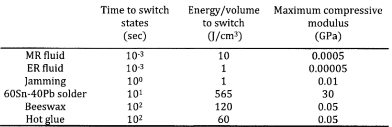
Table 1.1 presents a comparison of various phase-change and "smart" materials that are capable of transitioning between solid (or solid-like) and liquid (or liquid-like) states. The performance metrics compared are: the amount of time it takes to switch between

compressive modulus of the material in its most rigid state. Note that the values listed are meant to be order-of-magnitude approximations only, as some of the values depend on the mechanism employed to transition between states (e.g., an electromagnet or electro-permanent magnet can be used for MR fluid).

Table 1.1: A comparison of various phase-change and "smart" materials that are capable of transitioning between a solid (or solid-like) state and a liquid (or

liquid-like) state.

Time to switch Energy/volume Maximum compressive

states to switch modulus

(sec) (J/cm3_{) (GPa)} MR fluid 10-3 10 0.0005 ER fluid 10-3 1 0.00005 Jamming 100 1 0.01 60Sn-4OPb solder 101 565 30 Beeswax 102 120 0.05 Hot glue 102 60 0.05

From this brief survey of tunable strength and stiffness mechanisms, it was concluded that jamming of granular media exhibited a desirable combination of the metrics presented in Table 1.1. Therefore, jamming was selected as the mechanism to focus on for achieving variable strength and stiffness properties in soft robotic applications.

1.3 Jamming of granular media: background

This section provides a brief background of the research conducted in various disciplines-specifically, those outlining the spectrum in Figure 1.2-in the context of jamming and how it can be applied in real-world systems. The spectrum includes physics at one end, where decades' worth of fundamental granular studies have been conducted but often with idealized conditions; jamming applications at the opposite end, where engineers are developing novel systems that utilize jamming but with limited knowledge about how granular properties correlate with the performance of real-world systems; and soil mechanics in the middle, where both fundamental and empirical studies have been conducted in order to enable engineers to properly design geotechnical systems, which are often relatively large-scale and composed of natural materials.

1.3.1 Physics

"Jamming" is defined by the physics community as occurring when "force chains" are present such that local yield stresses are introduced in a system that can otherwise behave like a fluid, thereby enabling systems to transition between fluid-like and solid-like states [1][30]. The effective phase transition that occurs in jammed systems is analogous to what is observed in microscopic systems with attractive particle interactions [1][31][32]. Jamming, or when the effective solid phase is achieved, can occur only when the density of

particles exceeds a threshold. As seen in many materials at the microscopic scale, systems can become unjammed, or achieve the effective liquid phase, when the temperature is raised (e.g., when the system is vibrating) to a critical value or when the material is sheared enough to cause the particles to move relative to each other.

Significant work has been done in the physics community to understand how different grain parameters, such as shape and size distribution, affect system attributes including the jamming transition [33][34][35][36], packing fraction [37][38], and the distribution of force chains [39] [40] [41]. While these studies provide valuable insight into how grain properties might affect the performance of a system in a jamming application, they do not necessarily provide all the information that an engineer would need to make fully educated design decisions. For example, performance factors such as the bulk compressive stiffness and strength of a granular system as a function of confining pressure might be important to an engineer designing for a jamming application, though studies in the physics community do not necessary evaluate such metrics. Additionally, much of the research in the physics community focuses on idealized systems (e.g., frictionless spheres and infinite boundary conditions), which drastically differ from real-world systems.

1.3.2 Soil mechanics

Compared to the physics community, in which granular systems are typically limited to simple and idealized (e.g., frictionless) grains and boundary conditions, the soil mechanics community primarily conducts empirical studies on natural materials (mostly soils) for large-scale and long-term applications. For engineers developing jamming applications,

shape, surface roughness, and size distribution) and the correlation of grain properties with the bulk performance of systems (including the bulk compressive modulus and the bulk shear strength). As will be discussed further in Chapter 2, the soil mechanics community has conducted significant research to address the challenge of efficiently and accurately classifying properties of grains [42][43][44]. Additionally, engineers developing jammable systems greatly benefit from the breadth of research conducted to correlate such properties with the bulk performance of systems [45] [46] [47] [48].

While the soil mechanics community provides a vast knowledge base for those designing jammable systems, there are still many research challenges specific to jamming applications that need to be addressed. For example, how would the bulk performance of a granular system differ between a very large system under high confining stress (e.g., the foundation for a house) and a much smaller system under lower confining stress (e.g., a robotic manipulator on the scale of a human arm)? Another interesting challenge is, rather than being constrained to studying naturally occurring granular systems (as geotechnical engineers often are), how can engineers design and fabricate novel grains to fulfill a particular application's requirements? These questions motivate some of the work presented in this thesis.

1.3.3 Jamming applications

As previously mentioned, jamming of granular media is becoming increasingly popular across many areas because of its simplicity yet effectiveness in rapidly transitioning between relatively large ranges of strengths and stiffnesses. Figure 1.1 presents various examples of jamming applications from a range of fields, including robotics, user interfaces, medical technologies, and architecture. Even though one of the goals of the research presented in this thesis was to further the understanding of jamming in the field of robotics, we hope that our contributions will benefit many other fields as well.

Endioq

E) ( E)

endoscopic tube e stru ing & casting devi

Figure 1.3: A sampling of jamming applications across various fields. Applications include: a universal gripper [2][49]; a soft, mobile robot [50] [51]; tangible user interfaces [7]; an endoscopic tube [4]; architectural structures [5] [6]; and reconfigurable molding and casting

CHAPTER

2

RELATING GRANULAR PROPERTIES TO BULK

PERFORMANCE

1

2.1 Background and motivation

For many engineering applications, jammable components present opportunities that traditional rigid-body ones do not, as they can minimize the need for traditional rigid actuators, decrease costs, increase robustness, and increase range of motion. As previously mentioned, examples of novel jamming applications include a universal robotic gripper [2] [49], customizable architectural structures [5], a highly articulated robotic manipulator [3], a flexible endoscope [4], and tangible user interfaces [7].

Unfortunately, little headway has been made in identifying granular materials that are best suited for this new class of jammable systems. Isolated studies have been conducted to better understand how certain grain types affect system performance. In the case of the robotic manipulator, the strength-to-weight performance of six low-density materials was determined experimentally (as will be discussed in 4.3); for the endoscope, the bending stiffness of a slender jammable cylinder was determined for five candidate materials [4]; and in the development of a locomotive soft robot, an effective flexural

1 A significant portion of the data acquisition and analysis presented in this chapter was conducted by

students at The Massachusetts Institute of Technology in the Undergraduate Research Opportunities Program (UROP). Katy Gero conducted all the image data acquisition and analysis, and she also performed the initial set of direct shear tests discussed in this chapter. Sara Falcone also conducted direct shear tests, and Shaymus Hudson conducted the triaxial compression tests.

modulus as well as angle of repose was determined for five materials [51]. In total, the materials used in these studies were: different sized glass, acrylic, polystyrene, and steel beads; aluminum oxide particles (used for sandblasting); table salt; ground corncob; ground coffee; sawdust; diatomaceous earth; and granular corundum. While these selections represent educated guesses for suitable materials for jamming applications, they do not provide general information on what types of materials are optimal; these studies have yet to establish correlations between particle properties and jamming performance. The properties of the membrane also introduce important design parameters for jammable systems, and several groups have conducted preliminary studies to explore this design space [52][53].

For many jamming applications such as the ones described above, there are typically four properties that should be maximized to optimize the performance of the system:

1. the ease of which grains enter the solid-like state (for example, it would be difficult to arrange jigsaw-puzzle-like pieces to interlock);

2. the strength and/or stiffness of the system in the solid-like state; 3. the malleability of the system in the liquid-like state; and

4. the repeatability of these metrics across various jamming/unjamming cycles.

The goal of the work presented in this chapter is to correlate such "macroscopic" properties with "microstructure" granular ones-including grain shape, size distribution, and surface properties-to provide engineers with improved methods for selecting granular systems to best fulfill a particular application's requirements.

particle properties effective bulk properties

(microscopic, individual) (macroscopic, collective)

shape parameters mechanical properties

size distribution fluidity

surface properties ease of jamming

strength

predict

Figure 2.1: A visual representation of the goal of the work presented in this chapter, which is to correlate "microscopic" properties of individual grains with the "macroscopic"

performance of the bulk system.

This chapter presents experimental studies conducted on a wide range of materials with uncontrolled properties to identify whether there are any dominant "microscopic" grain properties that can be used to predict the "macroscopic" performance of granular systems. Specifically, from the categories listed in Figure 2.1, the macroscopic property of interest in these studies was the shear strength of grains, which is a mechanical property and can be quantified using a parameter called "friction angle" (described in further detail in 2.2). From the list of microscopic properties, it was hypothesized that grain shape and size distribution would dominate surface roughness in correlating the properties of individual grains to friction angle.

2.1.1 Characterizing "microscopic" grain properties: background

Describing the microscopic properties of a granular system using a single parameter is extremely difficult, as systems can vary, for example, in shape, size distribution and surface properties. Both researchers in the physics and soil mechanics communities have attempted to quantify grain descriptors, but studies are typically limited to subsets of materials that vary in a small number of aspects only (e.g., shape or size distribution). Because there has been a vast range of research in this area, this section provides only a brief introduction to the prior art and examples of common methods for characterizing grain properties in both 2D and 3D.

In 2D, simple parameters that are frequently used to approximate grain shapes include aspect ratio, circularity, and roundness [54] [42]. More complicated measurements, which usually aim at capturing small-scale features, such as roughness and surface texture, include methods such as fractal and Fourier analysis and discrete element modeling [55][43][56][57][58][59][60]. Grain size distribution has also been a metric of interest, as the ability for smaller grains to fill the voids of larger grains introduces interesting problems under topics including packing fraction and force-chain stabilization [38] [61]. As with the work presented in this chapter, many researchers in the soil mechanics community have been interested in how different grain properties might correlate with the macroscopic behavior of the system [46][47], though most of these studies are limited to soils, which do not necessarily cover the range of granular properties-including unusual shapes and surface properties-that might be represented in jamming applications.

Quantifying grain shapes in 3D is certainly more complicated than in 2D but could provide more useful information about the properties of grains. Many of the methods are similar to those used for 2D shapes, including sphericity and aspect ratio (of orthogonal axes). Additional methods include discrete element modeling [62].

2.2 Friction angle

Analogous to the coefficient of friction for sliding rigid bodies, the angle of internal friction, or friction angle, a, is a parameter that is related to the interparticle friction of grains and is used to predict the shear strength of granular systems. As with the coefficient of friction of sliding solids, friction angle is typically viewed as an intrinsic property because it represents the relationship between the shear and normal stresses in a granular system, which is expected to be linear within a range of confining stresses. Because most jamming applications utilize a vacuum pump to induce a differential jamming pressure, Piam, on the system, the possible range of confining pressures is approximately 0-101 kPa, as 101 kPa is ambient air pressure at sea level. As will be discussed, each of the materials studied in this chapter exhibited constant angles over this operational range of 0-101 kPa.

In the context of jamming applications, a large friction angle represents a large increase in shear strength as the confining pressure on the system (e.g., Pjam) increases, which is typically desirable for such applications.

2.3 Experimental methods and procedure

2.3.1 Grain selection

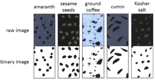
Due to their wide variety of grain properties-including shape, size distribution, and surface roughness-the majority of the materials tested in this chapter were organic grains that could be purchased at most supermarkets. To test the hypothesis that grain shape and size distribution dominate surface properties in predicting the macroscopic performance of materials, two of the grains tested-hulled and unhulled sesame seeds-were very similar except for surface texture.

An initial set of experiments was conducted on twenty-five materials, ten of which were later analyzed more thoroughly. This latter subset of materials covered a wide range of possible particle shapes, sizes, and surface properties.

2.3.2 Imaging analysis

Our studies focused on comparing grain properties that could be obtained from 2D silhouettes of grains using widely available imaging and analysis tools. 2D images of grains were acquired using various methods, depending on the features of the grain. To achieve silhouettes with maximum contrast, a macro-lensed, high-resolution DSLR camera was used to photograph large, opaque grains on a light table, while large, translucent grains were photographed on a black background. Smaller grains required greater magnification and were photographed using a light microscope.

With regard to 2D properties, it has been demonstrated that while shape descriptors derived from images from scanning electron microscopes (SEM) and light microscopes (LM) are slightly different, the relative comparisons among samples are similar [61]. Moreover, it has been demonstrated that LM images can provide accurate relative shape values rather than accurate absolute shape values, which is more important

when looking at shape profile characteristics as opposed to surface roughness characteristics.

ImageJ was used for the entire image analysis process for the results presented in this chapter; it is a java-based image-processing tool available on the public domain. In ImageJ, photos of grains were first converted to a binary format using an automatic conversion function. Examples of the converted images are presented in Figure 2.2. For the various grain properties considered, single values representing some geometric measurement or relation were calculated for every grain in each image using automatic functions.

sesame ground cumin Kosher

amaranth cumin

seeds coffee salt

raw image

binary image e04

0 4*

e e I

Figure 2.2: Example of raw and binary images of grains.

In the initial testing of twenty-five grain types, size distribution as well as several shape descriptors-including circularity, solidity, fractal dimension, and aspect ratio-were considered. After analyzing how these grain parameters varied with friction angle, we selected two parameters to focus further studies on: one shape factor, circularity, and one size distribution descriptor, polydispersivity. These parameters were selected because they yielded apparent correlations with friction angle (as will be discussed in 2.4), and they each also produced a large range of values relative to the measurement resolution for the grains that were tested. The shape descriptor circularity, C, was defined as:

41rA

C = (2.1)

where A and p were the projected 2D area and perimeter of each grain, respectively. The size distribution parameter polydispersivity, P, was defined as

P = Asta (2.2)

Amean

where Astd and Amean were the standard deviation and the mean values of 2D projected areas of grains from a large sample set, respectively. (Note that this definition of polydispersivity follows the definition of the "coefficient of variation," which is the ratio of the standard deviation to the mean values of a data set.)

With these parameters extracted from 2D information only, two main questions arose:

1. Can 2D silhouettes provide repeatable information about particle shape and size distribution, especially when considering non-axisymmetric grains?

2. What is the minimum number of grains that needs to be analyzed to accurately describe each material?

The first question was addressed experimentally: for each grain type, a large set of grains (on the order of hundreds to thousands) was photographed five times, each time after pouring and randomly distributing the grains onto a flat, horizontal surface. For each of the materials, the distribution of various grain properties (such as the cross-sectional area and perimeter of the grain silhouettes) in each photo remained reasonably constant across the five tests, indicating that 2D silhouettes can provide repeatable information about grain shape. Table 2.1 presents an example of select parameters extracted from ImageJ for a batch of ground coffee redistributed and photographed five times; note that, because a large number of grains was included in each batch of material, the majority but not necessarily all of the grains was photographed in each trial. Additionally, because grains would naturally settle in their most stable positions (e.g., sesame seeds would lie flat on horizontal surface rather than balancing on their thin edges), this method of photographing

2D silhouettes did not necessarily account for 3D properties that might be important for non-axisymmetric grains.

Table 2.1: An example of grain parameters extracted from ImageJ for a batch of ground coffee photographed five times, each time after randomly redistributing the

grains on a flat, horizontal surface.

Test no. Number of Average particle Average particle

particles recorded area circularity

(square pixels) (pixels)

1 2654 1583.1 2350.5 0.49 0.19

2 2198 1826.9 2546.5 0.51 + 0.19

3 2180 1656.9 + 2391.0 0.52 +0.19

4 1697 1835.5 + 2725.3 0.54 0.19

5 1686 1762.6+ 2470.4 0.56 0.18

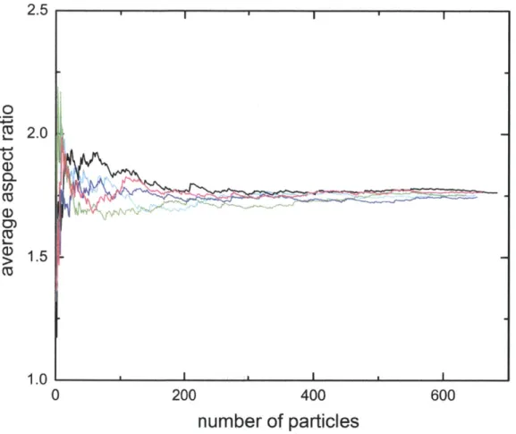
To address the second question, running averages of various shape descriptors were recorded to determine the minimum number of grains required to cause the running average to flatten. An example of this is presented in Figure 2.3, which plots the average aspect ratio vs. the number of particles considered (aspect ratio was calculated in ImageJ as the ratio of the major-to-minor axes of an ellipse fitted to a 2D silhouette of each grain). From this example, it was determined that approximately 400 grains of kosher salt were necessary to accurately describe the average aspect ratio of the material.

2.5 i i i 0 4-0CU 2.0-C5 CU

(,

number of particles

Figure 2.3: The running average for the parameter "aspect ratio" vs. the number of particles considered for kosher salt grains; each of the five curves represents a unique

distribution of grains in a single photograph.

2.3.3 Direct shear tests

Primarily used in the field of soil mechanics, there are various widely used experimental methods for determining friction angle, and while they typically yield similar trends when comparing different materials, they do not necessarily yield the same results for a given material due to the varying nature of different types of experiments [63]. Therefore, we were more interested in presenting an analysis of the resulting trends rather than the absolute friction angle values. For the results in this chapter, direct shear tests were conducted to determine the friction angle of grains. Triaxial tests were also conducted on a few of the materials to spot-check for any large discrepancies between the trends resulting from the two types of experiments.

normal load

force sensor

sample]

horizontal +shear plane displacement

force sensor

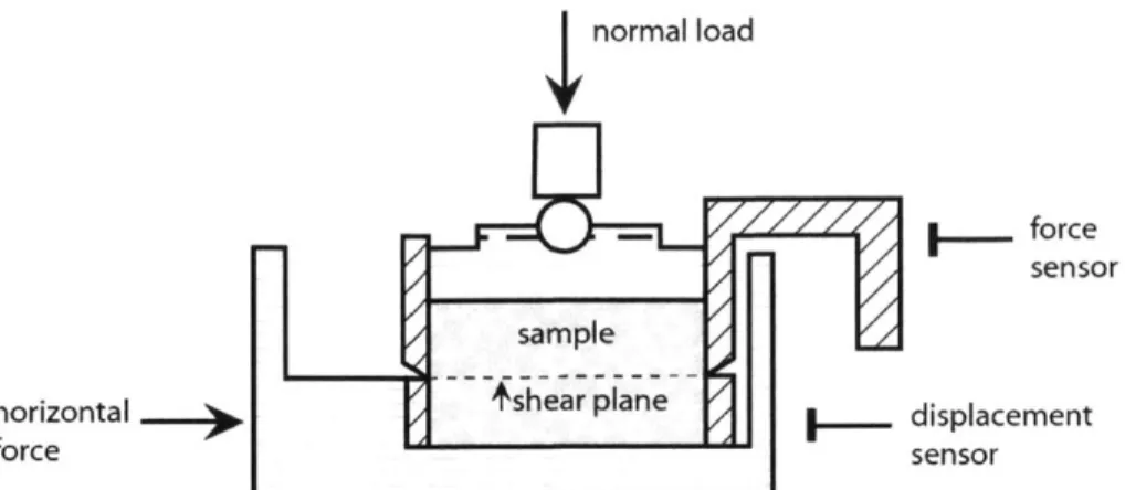
Figure 2.4: A schematic of the direct shear test set-up.

For the direct shear test, grains were placed in a vertically segmented box; a schematic of the set-up is presented in Figure 2.4. The cross section of the box was 6 cm x 6 cm and the height of the box was 5 cm (though the samples did not necessarily fill the height of the box). The lower section of the box was pushed horizontally at a fixed displacement rate to induce a horizontal shear plane in the sample, while the top section of the box was fixed. The resulting horizontal force that the top section experienced was used to calculate the shear stress of the material. For each material, a series of direct shear tests was conducted so that the maximum shear stress could be determined for different applied normal loads (which could be varied across tests but were held constant during each test), which were perpendicular to the direction of shearing. For reference, the mass of the samples ranged from 0.03 to 0.1 kg. A sample output of shear stress vs. horizontal displacement is presented in the inset of Figure 2.5 for three different applied normal loads.

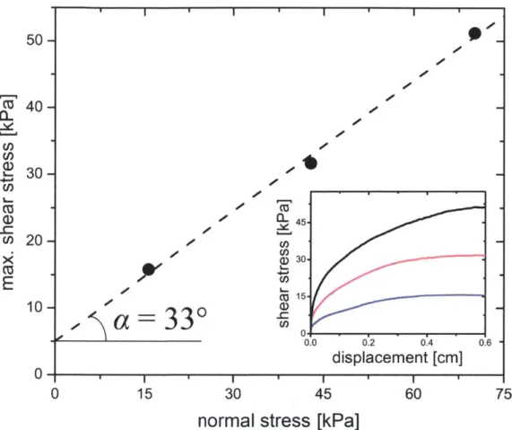
Figure 2.5 also presents an example plot (averaged over five trials) of maximum shear stress vs. applied normal load, which is expected to exhibit a linear relationship. Note that the standard deviation error bars for the maximum shear stress were so small that they do not extend beyond the markers in the plot. The slope of this curve is defined as the friction angle, a, of the material.

I * I 50- 300-(n 40 - - 30-1 --CL) Cl) (DOl_ 13467 (U C

E

normal stress [kPa]

Figure 2.5: An example of results from direct shear tests for ground coffee. The inset graph

presents the shear stress vs. displacement data for three different applied normal loads. The main graph presents the maximum shear stress versus the applied normal load. This latter curve is expected to be linear, and its angle relative to the horizontal axis is defined as the friction angle, a, of the material. Note that a non-zero vertical intercept in the main plot indicates that the material exhibits cohesion (i.e., the curve for cohesionless materials

would intersect the origin).

Five complete trials (each with the same set of three normal loads) were conducted for every material. Because the sample preparation procedure allowed for significant variability in how the grains were distributed into the box, a protocol was developed: grains were "loosely packed" into the box by pouring them through a funnel to incrementally and gradually control the distribution of material. In addition, previous studies have demonstrated that having different technicians conduct experiments can lead to inconsistent experimental results [64]. Therefore, for the work presented here, the same technician ran a majority of the experiments to maximize the precision of the results.

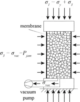
2.3.4 Triaxial tests

In addition to direct shear tests, triaxial compression tests-another common experiment in geotechnical engineering for determining friction angle-were also conducted on several materials to spot-check whether resulting trends varied significantly between the two types of experiments. While triaxial tests have a number of advantages over direct shear tests, namely that there are fewer stress concentrations at the boundaries and there is no forced failure plane in the material, they are more complex to conduct [63].

+

membrane

vacuum pump

Figure 2.6: A schematic of the triaxial test set-up used to determine the friction angle, a, of a set of grains, which were contained in a cylindrical, thin elastic membrane sealed off by

two rigid end plates. Labeled parameters: isotropic confining pressure 03, which is the vacuum pressure (ovac) applied to the inside of the cell; and a, which is equal to the sum

of the axial yield stress (ay) and the confining vacuum pressure. ai and a3 are the

-P 7 -I (3

3 jam IY

Figure 2.7: A schematic describing how the Mohr-Coulomb failure criterion is used to determine the friction angle, a, of a set of cohesionless grains. Note that a is expected to

remain constant for a limited range of a3 values (or confining pressures).

For the triaxial tests, granular samples were contained in a thin, cylindrical latex membrane, as illustrated in Figure 2.6. The triaxial samples were approximately 50-mm in diameter and 90-mm tall, and membranes were approximately 70-microns thick. Granular samples were "loosely packed" into the membrane by dispensing the material through a funnel in a circular motion to ensure a uniform distribution of material. During this process, the membrane was suctioned onto an outer rigid shell to maintain the desired shape of the specimen; the shell had two halves so that it could be easily removed prior to the experiment without disturbing the sample.

During each triaxial test, the specimen was subjected to an isotropic stress,

q3 = Pam (by using a vacuum pump to control the pressure inside the membrane), as well

as uniaxial loading. Friction angle was computed using Mohr's circle, with the two principal stresses being the applied isotropic stress, a3 = Pam, and the sum of the isotropic stress

and the compressive yield stress, a1 = Uy + Pam, respectively. As shown in Figure 2.7,

friction angle, a, was defined as the angle between the horizontal axis and the line that is tangent to the circle and intersects the origin (for cohesionless materials). Typically, for a limited range of q₃ initial conditions, a single line that tangentially intersects multiple

Mohr's circles should be used to calculate the friction angle of the material; therefore, materials that exhibit cohesion would yield an average tangent line with a non-zero vertical intercept.

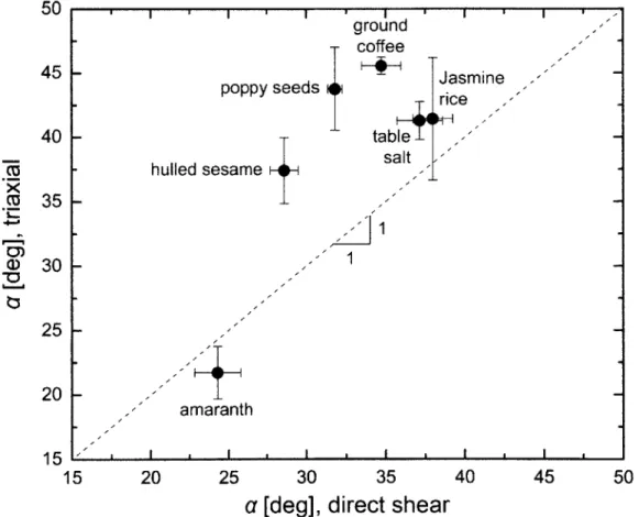
2.3.5 Direct shear vs. triaxial tests

A comparison of friction angle as determined from triaxial compression tests vs. direct shear tests is presented in Figure 2.8. From this comparison, it was concluded that the trends-but not the absolute values-resulting from the two types of experiments were comparable for the subset of materials tested. Direct shear tests generally yielded smaller friction angle values, which might be attributed to the test method's forced shear plane, causing the material to fail before it would under more natural conditions.

The friction angle data presented in the remainder of this chapter was determined from direct shear tests.

, . e poppy seeds hulled sesame

+

a [deg], direct shear

Figure 2.8: A comparison of friction angle, a, as determined from triaxial compression tests vs. direct shear tests. The dotted line with a slope of one serves as a visual aide to compare

how a differs between the two types of experiments (if the results between the two experiments were identical then all the points would lie on this line).

50 45

2.4 Results and discussion

2.4.1 Circularity and polydispersivity vs. friction angle

Figure 2.9 and Figure 2.10 present experimental results for (the inverse of) circularity and polydispersivity vs. friction angle, respectively. These results indicate an asymptotic-approach relationship between each of the two microscopic grain parameters and the macroscopic property, friction angle. For both cases, (2.3) was used to fit the data using a tangent function:

a = a tan~1 b (2.3)

where x was the microscopic grain parameter (C-' or P), and a, b, and c were fitting parameters. For circularity, the values for the fitting parameters were: a = 23.45 + 1.06, b = 0.015 + 0.02, and c = 1.15 ± 0.02, and the coefficient of determination was R = 0.66. For polydispersivity, the values for the fitting parameters were: a = 23.44, b = 0.008 0.009, and c = 0.14 + 0.03, and the coefficient of determination was R2 = 0.26.

This analysis indicates that circularity yielded a more reliable correlation with friction angle than polydispersivity did, though additional experiments should be conducted with materials that exhibit 0.5 P 5 1.4 in order to utilize a denser distribution

of P values to conduct a more thorough analysis of whether polydispersivity can be used to reliably predict friction angle. Regardless, the results provide insight when selecting a granular material for a given application because beyond a certain value of C-1 - 1.3 or

P ~ 0.3, there appears to be diminishing returns with increasing C-1 or P. This has

important implications when considering additional bulk properties such as the fluidity of the system in the unjammed state. One might expect that as C-1 increases, the fluidity of the system in the liquid-like state would decrease; as grains diverge from being spherical, their individual degrees of freedom (especially in rotation) are decreased, thereby inhibiting the motion of grains relative to each other to increase the resistance to bulk deformation [39][65]. Therefore, it would be ideal to utilize a grain that can transition between exhibiting a large value of C-1 for high shear strength in the solid-like state and a

small value of C1 _{for low shear strength in the liquid-like state. This concept of designing}

granular systems to have tunable properties is further explored in Chapter 3.

20 L.

1.0 1.5 2.0 2.5

C1

Figure 2.9: Friction angle, a, vs. the inverse of circularity, C 40

35

t 30

40

35 ~ _{ground coffee}

corn grit seed + hulled sesame

0 30 25 T amaranth 20 0.2 0.4 0.6 0.8 1 P

Figure 2.10: Friction angle, a, vs. polydispersivity, P

While circularity and polydispersivity appear to be correlated with friction angle, it is important to keep in mind that other factors, such as surface properties, can also have a significant influence on grain strength. A brief discussion about the two types of sesame seeds hypothesized to mostly differ in their surface properties is presented in 2.4.3.

2.4.2 Density vs. friction angle

For the direct shear tests, it was important to measure the density of the samples in the box in order to ensure consistent initial conditions. Additionally, for many jamming applications, the density of the grains can be an important consideration, especially for load-bearing applications, such as robotic manipulation, in which the strength-to-weight performance is a crucial factor. For example, while table salt exhibited a relatively large friction angle, it is relatively dense and might be a poor choice of material if the weight of the system were an important design parameter. The strength vs. weight performance of