HAL Id: hal-01429292
https://hal.archives-ouvertes.fr/hal-01429292v3
Submitted on 5 Sep 2017
HAL is a multi-disciplinary open access
archive for the deposit and dissemination of
sci-entific research documents, whether they are
pub-lished or not. The documents may come from
teaching and research institutions in France or
L’archive ouverte pluridisciplinaire HAL, est
destinée au dépôt et à la diffusion de documents
scientifiques de niveau recherche, publiés ou non,
émanant des établissements d’enseignement et de
recherche français ou étrangers, des laboratoires
Implementation of Discontinuous Skeletal methods on
arbitrary-dimensional, polytopal meshes using generic
programming
Matteo Cicuttin, Daniele Di Pietro, Alexandre Ern
To cite this version:
Matteo Cicuttin, Daniele Di Pietro, Alexandre Ern. Implementation of Discontinuous Skeletal
meth-ods on arbitrary-dimensional, polytopal meshes using generic programming. Journal of
Computa-tional and Applied Mathematics, Elsevier, 2018, 344, pp.852-874. �10.1016/j.cam.2017.09.017�.
�hal-01429292v3�
Implementation of Discontinuous Skeletal methods on
arbitrary-dimensional, polytopal meshes using generic
programming
M. Cicuttin, D. A. Di Pietro, A. Ern
September 5, 2017
Abstract
Discontinuous Skeletal methods approximate the solution of boundary-value problems by attaching discrete unknowns to mesh faces (hence the term skeletal) while allowing these dis-crete unknowns to be chosen independently on each mesh face (hence the term discontinuous). Cell-based unknowns, which can be eliminated locally by a Schur complement technique (also known as static condensation), are also used in the formulation. Salient examples of high-order Discontinuous Skeletal methods are Hybridizable Discontinuous Galerkin methods and the recently-devised Hybrid High-Order methods. Some major benefits of Discontinuous Skeletal methods are that their construction is dimension-independent and that they offer the possi-bility to use general meshes with polytopal cells and non-matching interfaces. In this work, we show how this mathematical flexibility can be efficiently replicated in a numerical software using generic programming. We describe a number of generic algorithms and data structures for high-order Discontinuous Skeletal methods within a “write once, run on any kind of mesh” framework. The computational efficiency of the implementation is assessed on the Poisson model problem discretized using various polytopal meshes and the Hybrid High-Order method.
1
Introduction
Discontinuous Skeletal (DiSk) methods are based on discrete unknowns that are discontinuous poly-nomials on the mesh skeleton. Additional cell-based unknowns are generally considered as well in the formulation of the method; such unknowns can be eliminated locally by a Schur complement technique (often referred to as static condensation in the finite element context). Eliminating the cell-based unknowns then leads to a global transmission problem coupling the face-based unknowns by means of a local stencil involving only adjacent elements in the sense of faces. DiSk meth-ods present several attractive features: the mathematical construction is dimension-independent, arbitrary polynomial orders can be used, and general meshes, including polytopal cells and non-matching interfaces, are supported. Positioning unknowns at mesh faces is also a natural way to express locally in each mesh cell the fundamental balance properties satisfied by the boundary-value problem at hand.
Seminal instances of lowest-order discretization methods placing unknowns at mesh faces are the Mimetic Finite Difference (MFD) methods (see [9] and the book [7]) and the Hybrid Finite Volume (HFV) methods (see [24] and the unifying approach with MFD in [22]); see also the Cell
Boundary Element (CBE) method in [29]. Perhaps one of the most well-known high-order DiSk methods are the Hybridizable Discontinuous Galerkin (HDG) methods introduced in [14] (see also the review in [11] and the references therein); we also mention the Generalized CBE method in [28]. Another prominent example of DiSk methods are the Hybrid High-Order (HHO) methods, which were recently introduced and analyzed in [16] for linear elasticity and in [18] for scalar diffusion, see also the mixed formulation in [17] and the recent review in [19]. HHO methods are currently undergoing a vigorous development, see, among others, their extensions to advection-diffusion [15], Stokes [20], Cahn–Hilliard [10], and Biot’s poroelasticity [8] equations. HHO methods have been recently bridged to HDG methods in [12], where a numerical flux trace for HHO methods has been identified in the context of a diffusion model problem. The three major differences between HDG and HHO methods are that HHO methods (i) are derived directly from the primal formulation, (ii) reconstruct locally the flux in a smaller space (exploiting its representation as the gradient of a potential) and (iii) deploy a (rather subtle) stabilization which achieves higher-order convergence rates on general meshes even when using simple polynomial spaces for the discrete unknowns (in contrast, similar properties for HDG methods generally require an enrichment of the underlying polynomial spaces, see, e.g., the recent work in [13]). Other examples of recent methods placing unknowns at mesh faces are the nonconforming Virtual Element method in [3] (which has been bridged to the HHO method in [12]) and the Weak Galerkin method in [32] (which has been bridged to HDG in [11]).
DiSk methods are devised at the mathematical level in a dimension-independent and cell-shape-independent fashion. The implementation, at least in principle, should reproduce this feature: a single piece of code should be able to work in any space dimension and to deal with any cell shape. It is not common, however, to see software packages taking this approach. In the vast majority of the cases, the codes are capable to run only on few very specific kinds of mesh, or only in 1D or 2D or 3D. On the one hand, this can happen simply because a fully general tool is not always needed. On the other hand, the programming languages commonly used by the scientific computing community (in particular Fortran and Matlab) are not easily amenable to an implementation which is generic and efficient at the same time. The usual (and natural) approach, in conventional languages, is to have different versions of the code, for example one specialized for 1D, one for 2D and one for 3D applications, making the overall maintenance of the codes rather cumbersome. The same considerations generally apply to the handling of mesh cells with various shapes, i.e., codes written in conventional languages generally support only a limited (and set in advance) number of cell shapes.
Generic programming [2] offers a valuable tool to address the above issues. Different libraries are already using such an approach to different extents; we mention, among others, [4, 6, 21, 27, 30, 31]. What generic programming provides is the possibility to write code where the data types are not immediately specified, but they are left as parameters. For example, a sort function written in generic style will not make any assumption neither on the data it will sort nor on the structure that contains data. Generic programming can be used also in a numerical code: by writing the code generically, it is possible to avoid making any assumption neither on the dimension (1D, 2D, 3D) of the problem, nor on the kind of mesh. In some sense, writing generic code resembles writing pseudocode: the compiler will take care of giving the correct meaning to each basic operation. As a result, with generic programming there will still be different versions of the code, but they will be generated by the compiler, and not by the programmer. As these considerations suggest, generic programming is a static technique: if correctly realized, the abstractions do not penalize the performance at runtime, because they will leave no trace in the generated code.
In the present work, we discuss a set of generic tools that can be used to implement DiSk methods, with a particular focus on HHO methods. The tools include a generic data structure to represent the discrete geometry (the mesh) and a set of operations on it. The data structure, which is composed of a three-layer abstraction, allows the user to handle simply “cells” and “faces” without having to care about what they really are (since the answer to this question depends on the ambient space dimension and the shape of the cell). To achieve this goal, the first layer hides the low-level details of a particular mesh format, and allows one to manipulate different “shapes” without caring about where they did come from and how they were originally represented. The second layer of abstraction hides the information about the shape of the cells and faces, but preserves the information about the dimension. Finally, the third layer hides the information about the dimension, presenting to the user just the concepts of cell and face. At this point, no matter what cells and faces actually are, it is possible to manipulate them in a unified and consistent way, and to obtain, at the same time, fine-tuned executable code.
This paper is organized as follows. In Section 2, we present the HHO method that we use as our main example among DiSk methods. We recall the functional formulation of the HHO method and, as a more practically-oriented presentation, we also describe its algebraic formulation (see also [1] for an algebraic presentation of the hybridized mixed HHO method). For simplicity, we focus on a simple model elliptic problem: the Poisson problem posed on a polytopal domain of Rd with homogeneous Dirichlet boundary conditions. In Section 3, we describe a generic implementation of DiSk methods on arbitrary-dimensional polytopal meshes. We first consider the various levels of abstraction necessary to handle mesh data structures in this context. Then we describe how various queries on the mesh can be implemented in this framework. In Section 4, we present a profiling of the implementation of the HHO method using the approach of Section 3 on a model elliptic problem using various two- and three-dimensional polytopal meshes. Finally, in Section 5, some conclusions are drawn.
2
An example: The HHO method
The goal of this section is to illustrate both the functional and the algebraic formulations of the HHO method when used to approximate the Poisson problem with homogeneous Dirichlet boundary conditions. Let Ω ⊂ Rd, d ≥ 1, be an open, bounded, connected, strongly Lipschitz set in Rd. For simplicity, we assume that Ω is a polygon/polyhedron. We want to approximate the weak solution u ∈ H01(Ω) such that
(∇u, ∇v)Ω= (f, v)Ω, ∀v ∈ H01(Ω), (1)
where (⋅, ⋅)Ωdenotes , according to the context, the standard inner product ofL2(Ω) orL2(Ω; Rd), and we assume for simplicity thatf ∈ L2(Ω).
2.1
Functional formulation
This section describes the functional formulation of the HHO method to approximate the model problem (1); for other boundary conditions, we refer the reader to [19]. This formulation has been introduced in [16, 18] hinging on two key operators, the reconstruction and the stabiliza-tion operator that are recalled below. We denote by T a mesh of Ω consisting of open disjoint polygonal/polyhedral cells with planar faces such that Ω = ⋃T ∈T T . A generic mesh cell is denoted
T ∈ T . We say that any subset F ⊂ Rd is a mesh face if it is a subset with nonempty relative interior of some affine hyperplane HF and if either there are two distinct mesh cells T1, T2 ∈ T so thatF = ∂T1∩∂T2∩HF and F is called an interface, or there is one mesh cell T ∈ T so that F = ∂T ∩ ∂Ω ∩ HF andF is called a boundary face. By construction, mesh faces are closed subsets of Rdand have mutually disjoint interiors. The mesh faces are collected in the set F , interfaces in the set Fi, and boundary faces in the set Fb. For allT ∈ T , let F∂T collect the mesh faces that are subsets of∂T . Note that we have {x ∈ ∂T } = ⋃F ∈F∂T{x ∈ F } and ⋃T ∈T{x ∈ ∂T } = ⋃F ∈F{x ∈ F }.
In what follows, (⋅, ⋅)T and (⋅, ⋅)F denote theL2(T )- and L2(F )-inner products for all T ∈ T and allF ∈ F, respectively. The same notation is used for the inner products of L2(T )d andL2(F )d. Since DiSk methods only require mesh cells and faces (mesh edges and vertices are not needed), we generically denote the mesh as the pair M ∶= (T, F).
2.1.1 Local polynomial spaces
Let us fix a polynomial degreek ≥ 0. For each mesh cell T ∈ T , let Pk
d(T ) be the space composed of d-variate polynomials of degree at most k restricted to T . For each face F ∈ F∂T, the space Pkd−1(F ) is composed of the restrictions to F of the polynomials in Pkd(T ). Since the face F is planar by assumption, this space can be described as Pkd−1(F ) = Pkd−1○TF−1whereTF ∶Rd−1→HF is an affine bijective mapping and whereHF is the affine hyperplane in Rd supporting the faceF . The space Pkd−1(F ) is independent of the choice of TF; indeed, considering another affine bijective mapping ˆTF ∶Rd−1→HF, one can observe thatT−1F ○ ˆTF is an affine bijective mapping from Rd−1 onto itself, so that Pkd−1○ (T−1F ○ ˆTF) =Pkd−1 and hence Pkd−1○T−1F =Pkd−1○ ˆT−1F .
We define the piecewise polynomial space Pkd−1(F∂T) ∶= ⨉
F ∈F∂T
Pkd−1(F ), (2)
and we observe that an elementv∂T ∈Pkd−1(F∂T)is a collection of polynomials indexed by the faces of T , i.e., we have v∂T = (vF)F ∈F∂T where vF ∈ P
k
d−1(F ) for all F ∈ F∂T. Note that there is no matching condition enforced on the polynomialsvF at vertices (in 2D) or edges (in 3D) separating neighboring faces in F∂T. Then, for each mesh cellT ∈ T , the local discrete space is
UTk ∶=Pkd(T ) × Pkd−1(F∂T). (3)
2.1.2 Reconstruction operator
LetT ∈ T be a mesh cell. We define Pk+1∗d (T ) ∶= {q ∈ Pk+1d (T ) ∣ (q, 1)T =0} (any supplementary sub-space of the subsub-space spanned by the constant function in Pk+1d (T ) can be equivalently considered). The local reconstruction operatorRk+1T ∶UTk →Pk+1∗d (T ) is defined such that, for all (vT, v∂T) ∈UTk and allw ∈ Pk+1∗d (T ),
(∇Rk+1T (vT, v∂T), ∇w)T ∶= (∇vT, ∇w)T + ∑ F ∈F∂T
(v∂T−vT, ∇w⋅nT)F, (4) where nT is the unit outward normal toT . By the Riesz representation theorem in ∇Pk+1∗d (T ) for theL2
(T ; Rd)-inner product, this uniquely defines ∇Rk+1T (vT, v∂T)and, recalling the zero-average condition, alsoRk+1
The local reconstruction operatorRk+1
T is used to build the following bilinear form onUTk×UTk: a(1)T ((vT, v∂T), (wT, w∂T)) = (∇Rk+1T (vT, v∂T), ∇Rk+1T (wT, w∂T))T, (5) which mimics locally the bilinear form in the left-hand side of (1).
One can show that the local reconstruction operator Rk+1T enjoys a polynomial consistency property of order (k + 1). To formalize this property, let ΠkT and ΠkF denote the L2-orthogonal projectors onto Pkd(T ) and Pkd−1(F ), respectively. Let us then define the reduction map ITk ∶ H1(T ) → Uk
T so that, for a functionv ∈ H1(T ), the cell component of ITk(v) is the cell L2-orthogonal projection ΠkT(v) and the face components of Ik
T(v) are the face L2-orthogonal projections ΠkF(v), for allF ∈ FT. Then, the following consistency property holds:
∇Rk+1T (ITk(q)) = ∇q, ∀q ∈ Pk+1d (T ). (6)
2.1.3 Stabilization operator
For (vT, v∂T) ∈ UTk, the reconstructed gradient ∇Rk+1T (vT, v∂T) is not stable in the sense that ∇Rk+1
T (vT, v∂T) =0 does not necessarily mean that vT andv∂T are constant functions taking the same value. To restore stability, we introduce a stabilization operator that relates the cell and face polynomials at the boundary of T . We define the stabilization operator Sk
T ∶ UTk → Pkd−1(F∂T) such that, for all (vT, v∂T) ∈UTk, lettingrk+1T ∈Pk+1d (T ) be such that ∇rTk+1= ∇Rk+1T (vT, v∂T)and (rk+1T −vT, 1)T =0, we have
STk(vT, v∂T) ∶=Πk∂T(v∂T− (vT +rTk+1−ΠkTrTk+1)∣∂T), (7) where Πk∂T is the L2
-orthogonal projector onto Pkd−1(F∂T) acting on each face F ∈ F∂T as the projector ΠkF defined above. Using this stabilization operator, we build the following bilinear form onUk
T×UTk:
a(2)T ((vT, v∂T), (wT, w∂T)) = ∑ F ∈F∂T
h−1F(STk(vT, v∂T), STk(wT, w∂T))F, (8) wherehF denotes the diameter of the face F .
The design of the stabilization operator Sk
T by means of (7) ensures the following polynomial consistency property of order (k + 1):
STk(I k
T(q)) = 0, ∀q ∈ P k+1
d (T ). (9)
At the same time, the stabilization operator Sk
T achieves the following crucial stability property: Defining onUk
T the semi-norm
∣(vT, v∂T)∣21,T∶= ∥∇vT∥2T+ ∑ F ∈F∂T
h−1F∥v∂T −vT∥2F, (10) (so that ∣(vT, v∂T)∣1,T =0 if and only ifvT and v∂T are constant functions taking the same value), one can show that there is a uniform constantc1>0 so that
c1∣(vT, v∂T)∣21,T≤ ∥∇Rk+1T (vT, v∂T)∥2T + ∑ F ∈F∂T
h−1F∥STk(vT, v∂T)∥2F, (11) for allT ∈ T and all (vT, v∂T) ∈UTk. Finally, we notice that the simpler definition STk(vT, v∂T) ∶= Π∂Tk (v∂T −vT∣∂T)for the stabilization operator leads to STk(ITk(v)) = Πk∂T(v) − ΠkT(v)∣∂T for any functionv ∈ H1(T ) and thus only ensures the polynomial consistency property Sk
T(ITk(q)) = 0 for allq ∈ Pk
2.1.4 Discrete problem
Recall the notation M = (T, F) for the mesh. The local discrete spaces Uk
T, for all T ∈ T , are collected into a global discrete space
UMk ∶=UTk×UFk, (12)
where
UTk ∶=Pkd(T ) ∶= {vT = (vT)T ∈T ∣vT ∈Pkd(T ), ∀T ∈ T }, (13a) UFk ∶=Pkd−1(F ) ∶= {vF= (vF)F ∈F∣vF∈Pkd−1(F ), ∀F ∈ F}. (13b) Given a pairvM∶= (vT, vF)in the global discrete spaceUMk , for allT ∈ T , we denote by (vT, v∂T) its restriction to the local discrete space Uk
T, where v∂T = (vF)F ∈F∂T. We enforce strongly the
homogeneous Dirichlet boundary condition by considering the subspace
UM,0k ∶=UTk×UF,0k , (14)
where
UF,0k ∶= {vF∈UFk ∣vF ≡0, ∀F ∈ Fb}. (15) For allT ∈ T , we combine the bilinear forms built using the reconstruction and the stabilization operators into a single bilinear formaT onUTk×UTk such that
aT ∶=a(1)T +a(2)T . (16)
The discrete problem consists in seekinguM∶= (uT, uF) ∈UM,0k such that
aM(uM, wM) =`M(wM), ∀wM∶= (wT, wF) ∈UM,0k , (17) where aM(uM, wM) ∶= ∑ T ∈T aT((uT, u∂T), (wT, w∂T)), (18a) `M(wM) ∶= ∑ T ∈T (f, wT)T. (18b)
The construction of the discrete problem (17) corresponds to a standard cellwise assembly as in finite element methods. The convergence analysis performed in [16, 18] leads to energy-error estimates of orderhk+1 and toL2-error estimates of orderhk+2 if full elliptic regularity holds for the model problem.
Referring, e.g., to [19] for more details, we observe that the discrete problem (17) can be ef-ficiently solved in a two-step procedure. In the first step, one expresses the cell unknownsuT in terms of the face unknownsuF and the source term f by solving the following coercive problem: FinduT ∈UTk such that
aM((uT, 0), (wT, 0)) = `M(wT, 0) − aM((0, uF), (wT, 0)), (19) for allwT ∈UTk. This problem is easy to solve since the unknowns attached to distinct mesh cells remain uncoupled, which is reflected by the fact that the matrix in the left-hand side is block
diagonal; see the discussion in Section 2.2.4. In the second step, one solves the following coercive problem: FinduF∈UFk such that
aM((0, uF), (0, wF)) =aM((uT, 0), (0, wF)), (20) for allwF ∈UFk, whereuT ∈UTk results from (19). One can show that the discrete problem (20) is a global transmission problem that expresses the fact that, across each interfaceF ∈ Fi, the jump of the numerical normal flux trace is zero.
2.2
Algebraic formulation
In this section we introduce the local matricesA(1)T andA(2)T that are the algebraic counterparts of the bilinear formsa(1)T anda(2)T introduced above. The implementation of these matrices is further described in Algorithm 1 from this Subsection and in the Listings 7 and 8 from Subsection 3.2. Moreover, the entries of these matrices are computed with quadratures that are further described in Algorithm 2 from Subsection 3.2.2.
In what follows, we adopt the convention that the indexing of vectors and matrices starts from 0. For integersl ≥ 0 and n ≥ 0, we denote by Nl
n ∶= (
l+n
l ) the dimension of the space composed of n-variate polynomials of degree at most l. In what follows, we shall need the numbers Nk
d,Nd−1k , andNk+1
d , wherek is the polynomial degree used in the HHO method and d is the space dimension. 2.2.1 Local basis functions
LetT ∈ T be a mesh cell. We fix a basis {φT,i}0≤i<Nk+1 d of P
k+1
d (T ). To simplify the presentation, we assume that the basis functions are such that (i)φT,0is the constant function (i.e., this function spans the kernel of the gradient operator), (ii) {φT,i}0≤i<Nk
d is a basis of P
k
d(T ). Letting N∂T denote the number of faces composing the boundary ofT , we enumerate these faces from 0 to N∂T−1. For all 0 ≤m < N∂T, we fix a basis {ψFm,n}0≤n<Nd−1k of P
k d−1(Fm); it is natural to setψFm,n= ˆψn○T −1 Fm, where { ˆψn}0≤n<Nk d−1is a basis of P k d−1andTFm∶R d−1
→HFmis the above-introduced affine bijective
mapping from Rd−1 to the affine hyperplaneHFm supporting Fm in R
d. Then, a pair (uT, u∂T) ∈UTk can be viewed as a vector UT ∈RN
k T, with
NTk∶=Ndk+N∂T ×Nd−1k , (21)
in such a way that
uT = ∑ 0≤i<Nk
d
UT,iφT,i, (22)
andu∂T = (uFm)0≤m<N∂T where, for all 0 ≤m < N∂T,
uFm = ∑
0≤n<Nk d−1
UT,Nk
d+mNd−1k +nψFm,n, (23)
i.e., we order first the components of the polynomial attached to the cell and then, enumerating the faces composing the boundary ofT , we order the components of the polynomial attached to each face.
We define the cell mass matrixMT ∈RN
k d×N
k
d such that
and for all 0 ≤m < N∂T, the face mass matrix MFm∈R Nk d−1×Nd−1k such that MFm,nn′∶= (ψFm,n, ψFm,n′)Fm, 0 ≤n, n ′ <Nd−1k . (25)
All of the above mass matrices are symmetric positive definite. Finally, let us setN∗dk+1∶=Ndk+1−1. We define the stiffness matrixKT ∈RN∗dk+1×N∗dk+1 such that
KT,ij∶= (∇φT,i+1, ∇φT,j+1)T, 0 ≤i, j < N∗dk+1. (26) Note that alsoKT is a symmetric positive definite matrix.
The implementation of the HHO method requires the inversion of the local stiffness matrixKT to evaluate the reconstruction operator and of the local matricesMT and MFm, 0 ≤m < N∂T, to
evaluate the stabilization operator. These operations can be efficiently and robustly accomplished using the Cholesky algorithm. Notice that the cost of computing the Cholesky factorization of the mass matrices (an operation required to compute the stabilization term) is basically negligible with respect to the cost of factorizing the stiffness matrix for the computation of the reconstruction term. As a matter of fact, the factorization cost scales as the cube of the matrix size, and the mass matrices are related to polynomials of orderk whereas the stiffness matrix is related to polynomials of order (k + 1).
2.2.2 Reconstruction operator We define the rectangular matrixVT ∈RN
k+1
∗d ×NTk (whose block structure is depicted in Figure 1)
such that, for all 0 ≤i < Nk+1
∗d and all 0 ≤j < Ndk, VT,ij∶= (∇φT,j, ∇φT,i+1)T− ∑
0≤m<N∂T
(φT,j, ∇φT,i+1⋅nT)Fm, (27)
and for all 0 ≤i < Nk+1
∗d and allNdk≤j < NTk,
VT,ij∶= (ψFm,n, ∇φT,i+1⋅nT)Fm, (28)
where 0 ≤m < N∂T and 0 ≤n < Nd−1k are uniquely defined by the relationj = Ndk+mNd−1k +n. Then, defining the symmetric positive semidefinite matrix (whose block structure is depicted in Figure 2)
A(1)T ∶=VTKT−1VT, A(1)T ∈RN
k
T×NTk, (29)
where the superscript denotes the transpose of a matrix, we infer that
a(1)T ((vT, v∂T), (wT, w∂T)) =WTA(1)T VT, (30) for all (vT, v∂T), (wT, w∂T) ∈UTkwith components collected in the vectors VT and WT, respectively. In the implementation, the inverse ofKT is not computed, but only its Cholesky decomposition. The pseudocode describing the computation of the matrixA(1)T is detailed in Algorithm 1. 2.2.3 Stabilization operator
We define the rectangular matrixNT ∈RN
k
d×N∗dk+1 such that
VT = VT = N k +1 ⇤ d N k +1 ⇤ d Nk d Nk d NNd 1d 1kk NNd 1d 1kk
Figure 1: Graphical representation of the block structure of the matrix VT. It consists in a first column
related to the interior of an element and of a variable number of additional columns related to the faces of the same element.
N k T N k T
=
NTk NTk A(1)T A(1)T VV†T†T KK−1T−1T Nk ∗d Nk ∗d Nk ∗d Nk ∗d VT VT +1 +1Figure 2: Graphical representation of the computation of the matrix A(1)T . The product K−1
T VT is carried
Algorithm 1 Procedure used to compute the matrix of the reconstruction operator. We denote withintegrate() a pseudocode function that returns a list of pairs (Qp, Qw)of quadrature points Qpand weights Qw.
1: function BuildReconstructionOperator(T ) 2: initializeVT ∈RN∗dk+1×NTk with zeros
3: Q ← integrate(T ) 4: for (Qp, Qw) ∈Q do
5: for 0 ≤ i < N∗dk+1 do 6: for 0 ≤ j < Ndk do
7: VT,ij←VT,ij+Qw∇φT,j(Qp) ⋅ ∇φT,i+1(Qp)
8: for Fm∈f aces(T ) do
9: Q = integrate(Fm)
10: for (Qp, Qw) ∈Q do
11: for 0 ≤ i < N∗dk+1 do 12: for 0 ≤ j < Ndk do
13: VT,ij←VT,ij+Qw∇φT,j(Qp) ⋅ ∇φT,i+1(Qp)
14: for 0 ≤ i < N∗dk+1 do 15: for 0 ≤ n < Nd−1k do
16: j ← Ndk+mNd−1k +n
17: VT,ij←VT,ij+QwψFm,n(Qp)∇φT,i+1(Qp)⋅nT
18: RT ←K−1T VT
N k d 1 N k d 1 Nk d 1 Nk d 1 NNTTkk
-Nk T Nk T N⇤dk+1 N⇤dk+1 -MFm MFm CCFFmm Y 1:k+1 Fm Y1:k+1Fm RRTT Y0:k Fm Y0:k Fm CT M 1 T NTRT CT MT1NTRT Nk T Nk T Nk d Nk d N k d 1 N k d 1 SFm SFm=
Figure 3: Graphical representation of the computation of the matrix SFm.
and the rectangular matricesYFm∈R
Nk
d−1×Ndk+1, for all 0 ≤m < N∂T, such that
YFm,nj∶= (ψFm,n, φT,j)Fm, 0 ≤n < N
k
d−1, 0 ≤ j < Ndk+1. (32) It is convenient to extract the submatricesY0∶kFm,nj∈R
Nk d−1×Ndk andY1∶k+1 Fm,nj∈R Nk d−1×N∗dk+1 such that Y0∶kFm,nj∶=YFm,nj, 0 ≤n < N k d−1, 0 ≤ j < Ndk, (33a) Y1∶k+1Fm,nj∶=YFm,n(j+1), 0 ≤n < N k d−1, 0 ≤ j < N k+1 ∗d . (33b)
We also need the component matricesCT ∈RN
k d×N k T such that CT,ij∶=δij, 0 ≤i < Ndk, 0 ≤ j < NTk, (34) andCFm∈R Nk d−1×NTk, 0 ≤m < N∂T, such that CFm,nj∶=δn,j−Ndk−mNd−1k , 0 ≤n < N k d−1, 0 ≤ j < N k T, (35)
where theδ’s are Kronecker symbols. These matrices simply recover the components attached to the cell or those attached to a specific face from the full set of components of a vector in RNTk. Finally,
setting RT ∶=K−1T VT ∈ RN
k+1
∗d ×NTk for the matrix associated with the reconstruction operator, we
define, for all 0 ≤m < N∂T,
SFm∶=MFmCFm−Y 1∶k+1 Fm RT −Y 0∶k Fm(CT−M −1 T NTRT). (36)
The sequence of computations needed to computeSFm is depicted in Figure 3. Introducing the
symmetric positive semidefinite matrix A(2)T ∶= ∑ 0≤m<N∂T h−1FmS FmM −1 FmSFm, A (2) T ∈R Nk T×N k T, (37) we infer that a(2)T ((vT, v∂T), (wT, w∂T)) =WTA(2)T VT, (38) for all (vT, v∂T), (wT, w∂T) ∈UTkwith components collected in the vectors VT and WT, respectively.
2.2.4 Discrete problem
For any pairvM= (vT, vF)in the global discrete spaceUM,0k , its components using the polynomial bases attached to the mesh cells and faces are collected in a global component vector VM∈RN
k M,0
with
NM,0k ∶=dim(UM,0k ) =NT ×Ndk+NFi×Nd−1k , (39) where NT denotes the number of mesh cells and NFi the number of mesh interfaces. Then, the
algebraic realization of the discrete problem (17) is the linear system
AMUM=BM, (40)
where the unknown is the vector UM ∈RN
k
M,0 collecting the components of the discrete solution
uM, the system matrixAM is assembled in the usual finite element fashion so that AM= ∑
T ∈T
PT(A(1)T +A(2)T )PT, (41)
with the local matrices A(1)T and A(2)T defined in (29) and (37), respectively, while the restriction matrixPT ∈RN
k
T×NM,0k collects the components of a vector attached to a given mesh cell T ∈ T
(and inserting zeros for components attached to possible boundary faces), and the right-hand side vector BMis constructed in a similar manner from the linear form`M in (17).
As above, an efficient way of solving the linear system (40) consists of using a two-step procedure based on a Schur complement. Let us order for simplicity the components attached to cell unknowns first and then those attached to face unknowns. This induces the decomposition UM= (UT, UFi) with UT ∈ RN k T with Nk T = NT ×Ndk, and UFi ∈ RN k Fi with Nk Fi = NFi ×N k d−1. Similarly, the decomposition of the right-hand side vector is BM= (BT, 0) and that of the system matrix leads (with obvious notation) to four blocksAT T,AT Fi,AFiT, andAFiFi. Introducing a similar block
decompositions for the right-hand side vector BM, the system (40) rewrites ⎡ ⎢ ⎢ ⎢ ⎣ AT T AT Fi AFiT AFiFi ⎤ ⎥ ⎥ ⎥ ⎦ [ UT UFi] = [ BT 0 ]. (42)
Then, the algebraic realization of the cell-based problem (19) reads
AT TUT =BT −AT FiUFi, (43)
where the submatrix AT T is block-diagonal (each block having size Nk
d), and using (43), the algebraic realization of the global transmission problem (19) becomes
ASUFi= −AFiTA−1T TBT, (44)
with the Schur complement matrix
3
Generic implementation tools for HHO methods
In this section, we describe generic programming tools for the implementation of DiSk methods. We first present in Subsection 3.1 some tools related to the mesh data structure and the operations to be performed on the elements of the mesh such as quadratures. These tools have a relatively wide scope, and can actually be used to implement other methods than DiSk ones. They are in essence similar to the tools used in other libraries using generic programming to different ex-tents, as in [4, 6, 21, 27, 30, 31]. Then, in Subsection 3.2, we discuss generic programming tools that are more specific to DiSk methods. For simplicity, we focus on HHO methods as an illus-trative example, but the presentation can be adapted to other DiSk methods. We provide several (short) listings to illustrate the generic implementation. For further insight, the reader may consult the library, named DiSk++, which is available as open-source under MPL License at the address https://github.com/datafl4sh/diskpp.
3.1
Mesh data structure
Although our main focus is on DiSk methods for which only mesh cells and faces are the relevant geometric objects, we slightly broaden the discussion here so as to include mesh edges and vertices as well. For a d-dimensional mesh, the cells are its elements of dimension d and the faces are its elements of dimension (d − 1). We consider specifically cells that are d-polytopes (not necessarily convex) and their faces are planar. Before getting started, let us provide a simple example of the level of generality we want to achieve. The following listing describes how to implement in the present setting a function to compute the measures of all the mesh elements.
1 template<typename Mesh>
2 void list_measures(const Mesh& msh) 3 {
4 for (auto& cl : msh)
5 {
6 std::cout << measure(msh, cl) << std::endl;
7 auto fcs = faces(msh, cl);
8
9 for (auto& fc : fcs)
10 std::cout << " - " << measure(msh, fc) << std::endl;
11 }
12 }
Listing 1: The code of this listing is an example of the level of generality we want to achieve in our library. The code computes the measure of the mesh elements, and is suitable for any mesh.
3.1.1 Abstracting the various geometric entities
At the most basic level, a mesh is composed by different geometric entities having specific shapes: nodes, edges, triangles, quadrangles, tetrahedra, hexahedra and so on. Depending on the kind of the elements that a mesh contains, we can categorize the mesh as simplicial, hexahedral or - in
the most general cases - polyhedral. Keeping visible all the information about the exact kind of elements, however, would prevent us from achieving the desired level of generality. We therefore introduce three levels of abstraction:
Transforming the mesh file in an internal representation of “shapes”,
Mapping the “shapes” to generic nodes, edges, surfaces and volumes (n-polytopes with 0 ≤ n ≤ d),
Mapping d-polytopes to cells, (d − 1)-polytopes to faces, and so on.
Note that the role of the abstraction is to hide information, and not to discard it. This means that while writing code, the user does not care about what a cell or a face actually is, but the library at all times has the knowledge of all the details. Note also that we keep a representation for the various geometric mesh entities since in HHO methods for instance, mesh faces have to be handled independently of the mesh cells. Moreover, keeping a fully explicit mesh representation allows us to implement, in addition to DiSk methods, also discretization methods requiring the access to elements different than cells and faces (e.g., conforming finite elements).
First level of abstraction The first level of abstraction can be implemented in the loaders and in the storage classes. The role of a loader is to read a mesh file, find the “shapes” present in the mesh, and generate shape objects that have some representation (reflected in the code by specific types). That representation is dictated by the storage classes.
A storage class is a class tailored to encapsulate the representation of a specific kind of element (which we call physical element ) as efficiently as possible, exploiting the features of that element to optimize memory usage and computational speed. Various storage classes can be provided, for instance, simplicial element, the hexahedral element and generic element. Objects created from the simplicial element and hexahedral element storage classes are very lightweight and do not use dynamic memory, but they are limited in the kind of elements (and thus shapes) they can represent. On the other hand, objects created from the generic element class can handle any kind of element, but they require the usage of dynamic memory and are more expensive. Some performance comparison between the different storage classes will be shown in Section 4 below.
To summarize, with the first abstraction level, the details of all the different mesh file formats are hidden because elements are stored inside objects belonging to specific storage classes.
Second level of abstraction The second level of abstraction introduces the concepts of nodes, edges, surfaces and volumes. We will call these objects abstract mesh elements. The goal of the second abstraction layer is to map the abstract elements to the physical elements. For example, in the case of a simplicial mesh, surfaces are mapped to triangles and volumes to tetrahedra.
This mapping is established in the mesh storage, via the tag StorageClass (see Listing 2), which is required to instantiate the storage class trait and to retrieve the correct types of the physical elements. In this way, from the user’s point of view, a mesh storage is nothing more than a container for abstract elements; however, all the required information about the physical elements is retained in the proper way.
1 template<typename T, size_t DIM, typename StorageClass> 2 class mesh_storage /* Main template */
3 {
4 static_assert(DIM > 0 && DIM <= 3, "Only 1D, 2D and 3D"); 5 };
6
7 template<typename T, typename StorageClass>
8 struct mesh_storage<T, 3, StorageClass> /* 3D specialization*/ 9 {
10 typedef storage_class_trait<StorageClass, 3> sc_trait; 11 typedef typename sc_trait::volume_type volume_type; 12 typedef typename sc_trait::surface_type surface_type; 13 typedef typename sc_trait::edge_type edge_type; 14 typedef typename sc_trait::node_type node_type; 15
16 std::vector<volume_type> volumes;
17 std::vector<surface_type> surfaces;
18 std::vector<edge_type> edges;
19 std::vector<node_type> nodes;
20 };
Listing 2: Definition of the mesh storage. The 3D specialization is shown; the 2D specialization does not have the volumes member, while the 1D one has only the members nodes and edges.
The advantage of this structure is that, when a new kind of mesh has to be supported, the modifications to the code are very localized. To add the support for a new kind of elements, it is just needed to write:
The storage classes that encapsulate the implementation details of the new physical elements, The loader (or the loaders) for the new mesh format(s),
The trait specialization that specifies which are the actual types of the new physical elements. Third level of abstraction The third level of abstraction is obtained by a template called mesh, which (among other things) provides the methods to obtain the iterators on the cells and on the faces. The mesh template has three specializations, which correspond to the dimensions 1, 2 and 3; moreover, to be instantiated it needs also the type of the underlying storage. Thus, depending on the dimension, the methods of mesh that return the iterators on the cells and on the faces do nothing else than redirecting the call to the correct methods of its underlying storage. In other words, if cell iterators are requested on a 3D mesh, the call is redirected to the member volumes of the storage, while if face iterators of a 2D mesh are requested, the call is redirected to the member nodes of the underlying storage. For reasons of modularity and decoupling, this third level of abstraction is actually implemented by a hierarchy of three template classes: mesh bones, mesh base and mesh (see Figure 4). The user interacts only with mesh.
+mesh() … mesh +mesh_base() … priv::mesh_base +mesh_bones() … priv::mesh_bones +mesh_storage() … mesh_storage 1..1 0..1 Implementation details, not meant to be used by the user +loader() … loader Backend Fr ontend
Figure 4: UML (Uniform Modeling Language) diagram of the class hierarchy implementing the mesh data structure.
We emphasize that all the classes defined above (the storage and the classes of the mesh hier-archy) are fully generic. A mesh becomes polyhedral, hexahedral, simplicial only because of the StorageClass discussed before. Moreover, all the abstractions depend exclusively on static (i.e., compile time) information: this means that the implementation avoids the costs of dynamic method selection or other mechanisms found in object-oriented programming.
3.1.2 Queries on the mesh elements
An essential capability of the above generic programming tools is to enable queries about properties of the elements, like barycenter, volume, area and so on. Since the main goal is to provide a uniform interface across different kinds of meshes, the functions computing these quantities are templates parametrized on the type of the mesh and the type of the element.
Geometry-related queries The barycenter() function for example (see Listing 3) is parametrized in a way that matches any kind of mesh and any kind of element, since in every case the barycenter is computed by adding (coordinate-wise) all the points and by dividing by their cardinality.
1 template<typename Mesh, typename Element> 2 typename Mesh::point_type
3 barycenter(const Mesh& msh, const Element& elm) 4 {
5 auto pts = points(msh, elm);
6 auto bar = accumulate(next(pts.begin()), pts.end(), pts.front()); 7 return bar / typename Mesh::coordinate_type( pts.size() );
8 }
Listing 3: Computation of the barycenter
The measure() function, however, has different versions with parametrizations that match only specific kinds of meshes and elements.
1 template<typename T>
2 T measure(const generic_mesh<T,2>& msh,
3 const typename generic_mesh<T,2>::face& fc);
Listing 4: Prototype of the function that computes the measure for a 2D generic face
In Listing 4, the signature matches only 2D general meshes and in this case the function will compute and return a length. In Listing 5, however, the signature matches only the faces of a 3D simplicial mesh and then the corresponding function will compute and return an area.
1 template<typename T>
2 T measure(const simplicial_mesh<T, 3>& msh,
3 const typename simplicial_mesh<T, 3>::face& surf);
Listing 5: Prototype of the function that computes the measure for a 3D simplicial face
Different functions will therefore be called on different kinds of mesh, and the right function to use is selected at compile time by the compiler. This selection is based exclusively on information available statically to the compiler, and therefore has zero runtime overhead. To conclude, when the support for a specific operation has to be added to a new mesh format, it suffices to add the right function specialization.
Polynomials, basis functions and quadratures Polynomial basis functions and quadrature rules can also be made available as generic templates working on any kind of mesh. For instance, if one wants to compute the integral (p, q)T on all the elements of the mesh, withp, q ∈ Pkd(T ), one just needs the code shown in Listing 6, which is mesh-independent.
1 template<typename Mesh>
2 void compute_integrals(const Mesh& msh) 3 {
4 /* assumes that degree, p and q are correctly defined */ 5 typedef Mesh mesh_type; 6 typedef typename mesh_type::cell_type cell_type; 7
8 scaled_monomial_scalar_basis<mesh_type, cell_type> cb(degree); 9 quadrature<mesh_type, cell_type> cq(2*degree);
10 for (auto& cl : msh)
11 {
12 auto quadpoints = cq.integrate(msh, cl);
13 for (auto& qp : quadpoints)
14 {
15 auto phi = cb.eval_functions(msh, cl, qp.point());
16 mass_matrix += qp.weight() * phi * phi.transpose();
17 }
18
19 std::cout << "(p,q) = " << dot(q, mass_matrix*p) << std::endl;
20 }
21 }
Listing 6: Example of a function to compute an integral
3.2
Generic HHO Implementation
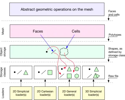
HHO methods only use mesh cells as faces. The overview of the mesh data structure for HHO methods is schematized in Figure 5.
The two key ingredients in HHO methods are the gradient reconstruction operator (correspond-ing to ∇Rk+1
T ) and the stabilization operator. To compute the gradient reconstruction operator, one can use the gradient reconstruction template, that can be instantiated as in Listing 7.
2D Simplicial
loader(s) 2D Cartesian loader(s) 2D General loader(s) 3D Simplicial loader(s) Cells Faces Faces and cells Polytopes Shapes, as defined by storage class Raw file Loaders Storage classes Object storage Mesh
Abstract geometric operations on the mesh
Figure 5: Overview of the mesh data structure for HHO.
1 gradient_reconstruction<mesh_type, 2 cell_basis_type, 3 cell_quadrature_type, 4 face_basis_type, 5 face_quadrature_type> gradrec(degree); 6 for (auto& cl : msh) 7 { 8 gradrec.compute(msh, cl);
9 // gradrec.oper contains the operator 10 // gradrec.data contains a(1)T
11 }
Listing 7: Gradient reconstruction operator declaration. The template implementing gradient reconstruc-tion must be instantiated specifying the type of the mesh, the types of the bases and the types of the quadratures. These parameters allow the compiler to specialize the operator to the specific kind of problem being solved. Then, the actual operator can be computed inside of the assembly loop by calling the method compute(), which is the counterpart of the pseudocode of Algorithm 1.
To compute the stabilization, one can use the diffusion like stabilization template, that can be instantiated as in Listing 8.
1 diffusion_like_stabilization<mesh_type, 2 cell_basis_type, 3 cell_quadrature_type, 4 face_basis_type, 5 face_quadrature_type> stab(degree); 6 7 for (auto& cl : msh) 8 { 9 stab.compute(msh, cl); 10 // stab.data contains a(2)T 11 }
Listing 8: Stabilization operator declaration. The stabilization operator, like the gradient reconstruction, must be instantiated specifying the type of the mesh, the types of the bases and the types of the quadratures.
There are similar template classes specific for the static condensation and for the assembler, that are omitted for brevity.
With all these classes instantiated, after loading the mesh with a specific loader that fills the msh object, the assembly phase of the problem reduces to the code described in Listing 9.
1 for (auto& cl : msh) 2 { 3 /* build a(1)T + a(2)T */ 4 gradrec.compute(msh, cl); 5 stab.compute(msh, cl, gradrec.oper); 6 7 auto cell_rhs =
8 disk::compute_rhs<cell_basis_type,
9 cell_quadrature_type>(msh, cl, load, degree);
10
11 /* local cell contribution: a(1)T + a(2)T */ 12 matrix_type loc = gradrec.data + stab.data; 13
14 /* do static condensation */
15 auto sc = statcond.compute(msh, cl, loc, cell_rhs); 16 assembler.assemble(msh, cl, sc);
17 } 18
19 assembler.impose_boundary_conditions(msh, bc_func); 20 assembler.finalize();
Listing 9: Assembly of the model diffusion problem using the HHO method.
has executed, the assembler object provides two members, matrix and rhs, that give access to the global linear system. These two members can then be passed to a suitable solver.
3.2.1 Choice of basis functions
As discussed in Section 2, we need polynomial basis functions associated with the cells and the faces of the mesh. In the results reported below, we used a basis composed of scaled monomials to generate them. Let ¯xT ∈Rd be the barycenter of the cellT , x ∈ T a point in T , and hT the diameter ofT defined as the maximal distance between two vertices. A scaled monomial is of the form
mT(x) = d ∏ i=1 ˜ xαi T,i, (46)
where ˜xT = (x− ¯xT)/hT and ˜xT,iis thei-th component of ˜xT. The scaled monomial basis for Pkd(T ) is formed by taking all the monomialsmT(x) of degree up to k:
Pkd(T ) = span { d ∏ i=1 ˜ xαi T,i∣1 ≤i ≤ d ∧ 0 ≤ d ∑ i=1 αi≤k} . (47)
One advantage of the above choice of basis functions is that the two quantities that depend onT (¯xT andhT) can be coded in a generic fashion, independent of the actual shape of the element.
Regarding the basis functions associated with the faces, since they are (d−1)-variate polynomials, we need to consider the affine bijective mappingTF ∶Rd−1→HF introduced in Section 2.1.1. To this aim, we introduce a local coordinate system on the faceF with origin at the barycenter xF and with local coordinates denoted by ξF = (ξF,i)1≤i≤d−1. This coordinate system is obtained by choosing (d − 1) edges of F with a vertex in common and such that they give rise to a set of linearly independent edge vectors (ki)1≤i≤d−1. These vectors are subsequently made orthonormal using the Gram–Schmidt process as originally proposed in [5] in the context of Discontinuous Galerkin methods. Given a pointx ∈ F , its local coordinates (ξF,i)1≤i≤d−1 are computed by first calculating the rescaled vector ˜xF = (x − ¯xF)/hF and then by projecting ˜xF on all the vectors ki. A scaled monomial is of the form
mF(ξ) = d−1 ∏ i=1 ξαi F,i. (48)
The scaled monomial basis for Pkd−1(F ) is finally formed by taking all the monomials mF(ξ) of degree up tok: Pkd−1(F ) = span { d−1 ∏ i=1 ξαi F,i∣1 ≤i ≤ d − 1 ∧ 0 ≤ d−1 ∑ i=1 αi≤k} . (49) 3.2.2 Quadratures
The code employs different quadratures, depending on the kind of element on which integration is required. On edges, standard Gauss quadrature is used. When integration on triangles and on tetrahedra is needed, the Dunavant quadrature [23] and the Grundmann–Moeller quadrature [26] are used respectively. If elements are quadrilaterals or hexahedra, the quadrature is obtained by tensorizing the one-dimensional Gauss quadratures. Finally, when the elements are polytopes that
are star-shaped with respect to their barycenter (as is the case for the meshes we consider), they are broken up into simplices and the integration is computed simplex by simplex. The appropriate quadrature is selected statically during the instantiation of the quadrature template. The efficiency of generic quadratures on elements for which specific quadratures are available (e.g., simplices) is guaranteed by a templated implementation resembling the pseudocode provided in Algorithm 2. Algorithm 2 Selection of appropriate quadratures. According to the data type of the cell, the compiler selects at compile time the appropriate quadrature method. The user however sees only one integrate() function. T etrahedralQuadratures(T ) and LineGaussP oints() are pseudocode functions returning sets of pairs of quadrature points and corresponding weights, as in Algorithm 1.
1: template<typename CellType> 2: function integrate(CellType T ) 3: Q ← ∅ 4: {S1, . . . , Sn} ←SplitInSimplices(T ) 5: for S ∈ {S1, . . . , Sn}do 6: Qs←T etrahedralQuadrature(S) 7: Q ← Q ∪ Qs return Q 8: template<> 9: function Integrate(TetrahedralCellType T ) 10: Q ← T etrahedralQuadrature(T ) return Q 11: template<> 12: function Integrate(CartesianCellType T ) 13: G ← LineGaussP oints() 14: Q ← T ensorizeGaussP oints(T, G) return Q
4
Profiling on a model elliptic problem
The goal of this section is to present a profiling of the generic programming tools described in Section 3. We profiled different parts of the library, in particular the computation of the recon-struction operator, the computation of the stabilization operator, the static condensation and the solver. DiSk++ uses the Eigen library for the linear algebra operations, at the time of writing Eigen 3.3.1 was available. For the solution of the linear system, we used the PARDISO sparse linear solver from the Intel MKL library. The reported timings represent the total time,tcpu, spent by the pro-gram on all the CPUs. Since the propro-gram was run on a 4-core CPU (Intel Core i7-3615QM), actual wall-clock times were much lower. We note that the assembly is sequential whereas the solver is run in parallel on 4 cores. The reported CPU times are as per getrusage(). The code has been compiled both with clang and gcc, and the usual optimization level is -O3.
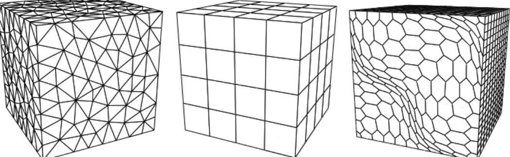
We have collected data about the running times on 2D triangular and hexagonal meshes and on 3D tetrahedral, hexahedral, and polyhedral meshes. The 3D meshes were obtained from the
FVCA6 benchmark [25]; some meshes are illustrated in Figure 6. The timings are reported against the total number of face-based components in the linear system, which we denote by DOFs, i.e.,
DOFs ∶=NFki =NFi×Nd−1k . (50)
The right-hand term we used to solve (1) was f = sin(πx) sin(πy) in the 2D case and f = sin(πx) sin(πy) sin(πz) in the 3D case, and the domain Ω was, respectively, the unit square and the unit cube. Chp. 8. Elliptic equations
Figure 8.5 – Coarsest mesh of each mesh sequence considered for numerical tests. From top
left to bottom right: Hex, PrT, PrG, HLR, CB, and Ker mesh sequences.
8.4.1 Postprocessed quantities
Quantities related to convergence. We compute discrete and continuous error norms
to evaluate the convergence rates of CDO schemes. Two generic discrete error norms are
considered: one based on the discrete functional norms and the other one induced by a discrete
Hodge operator.
Definition 8.39 (Discrete error norms). Let a œ S
X( ) be an exact solution of a diffusion
problem and let a œ X be the related discrete solution. Then, we set
Er
X(a) := |||R
X(a) ≠ a|||
2,X|||R
X(a)|||
2,X,
Er
–,X(a) := |||R
X(a) ≠ a|||
–,X|||R
X(a)|||
–,X.
(8.78)
We recall that the discrete norms |||·|||
2,Xand |||·|||
–,Xare defined in Section 6.1.
In what follows, we compute Er
V(p) and Er
Ÿ,E(g) to evaluate the discrete error on the
potential and its gradient in vertex-based schemes, Er
VÂ(p) and Er
Ÿ≠1,F(„) to evaluate the
discrete error on the potential and its flux in mixed cell-based schemes, and Er
VÂ(p) and
Er
úŸ,EÂ
(g) to evaluate the discrete error on the potential and its gradient in hybrid cell-based
schemes. The last discrete error is adapted from (8.78) as follows:
Er
ú Ÿ,EÂ(g)
2:=
q cœC|||R
EÂc(g) ≠ g
c|||
2Ÿ,EÂ c q cœC|||R
EÂc(g)|||
2Ÿ,EÂc,
(8.79)
where |||b
c|||
2Ÿ,EÂc:= vH˜
EcFcŸ(b
c), b
cw
Fc˜
Ecfor all c œ C and all b
cœ
E
Âc. Two continuous error norms
are also evaluated.
Definition 8.40 (Continuous error norms). Let a œ S
X( ) be an exact solution of a diffusion
problem and a œ X be the related discrete solution. Then, we set
Er
L2(a) := ||
a
≠ L
X(a)||
L 2( )||a||
L2( ),
Er
–(a) := ||
a
≠ L
X(a)||
–||a||
–,
(8.80)
where we recall that ||a||
2–
=
s
a
· – a.
Chp. 8. Elliptic equationsFigure 8.5 – Coarsest mesh of each mesh sequence considered for numerical tests. From top
left to bottom right: Hex, PrT, PrG, HLR, CB, and Ker mesh sequences.
8.4.1 Postprocessed quantities
Quantities related to convergence. We compute discrete and continuous error norms
to evaluate the convergence rates of CDO schemes. Two generic discrete error norms are
considered: one based on the discrete functional norms and the other one induced by a discrete
Hodge operator.
Definition 8.39 (Discrete error norms). Let a œ S
X( ) be an exact solution of a diffusion
problem and let a œ X be the related discrete solution. Then, we set
Er
X(a) := |||R
X(a) ≠ a|||
2,X|||R
X(a)|||
2,X,
Er
–,X(a) := |||R
|||R
X(a) ≠ a|||
–,X X(a)|||
–,X.
(8.78)
We recall that the discrete norms |||·|||
2,Xand |||·|||
–,Xare defined in Section 6.1.
In what follows, we compute Er
V(p) and Er
Ÿ,E(g) to evaluate the discrete error on the
potential and its gradient in vertex-based schemes, Er
ÂV(p) and Er
Ÿ≠1,F(„) to evaluate the
discrete error on the potential and its flux in mixed cell-based schemes, and Er
ÂV(p) and
Er
úŸ,EÂ
(g) to evaluate the discrete error on the potential and its gradient in hybrid cell-based
schemes. The last discrete error is adapted from (8.78) as follows:
Er
ú Ÿ,EÂ(g)
2:=
q cœC|||R
EÂc(g) ≠ g
c|||
2 Ÿ,EÂc q cœC|||R
EÂc(g)|||
2Ÿ,EÂc,
(8.79)
where |||b
c|||
2Ÿ,EÂ c:= vH˜
EcFcŸ
(b
c), b
cw
Fc˜
Ecfor all c œ C and all b
cœ
E
Âc. Two continuous error norms
are also evaluated.
Definition 8.40 (Continuous error norms). Let a œ S
X( ) be an exact solution of a diffusion
problem and a œ X be the related discrete solution. Then, we set
Er
L2(a) := ||
a
≠ L
X(a)||
L 2( )||a||
L2( ),
Er
–(a) := ||
a
≠ L
X(a)||
–||a||
–,
(8.80)
where we recall that ||a||
2–
=
s
a
· – a.
Figure 6: Examples of tetrahedral, hexahedral, and polyhedral meshes from the FVCA6 benchmark used in the tests.
4.1
2D test cases
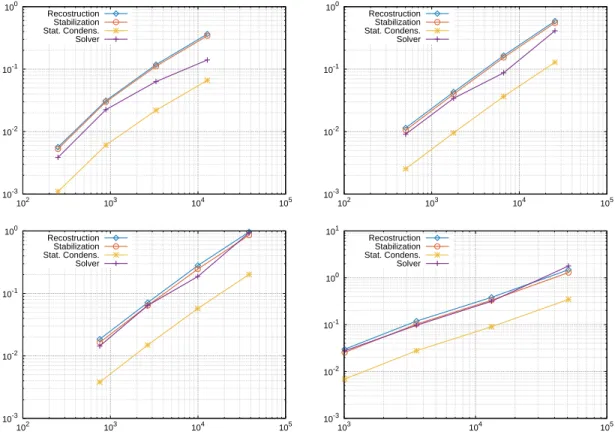
The 2D test cases were run on triangular and hexagonal meshes. The triangular meshes have 56, 224, 896, and 3584 elements respectively, whereas the hexagonal meshes have 76, 280, 1072, and 4192 elements respectively. In Figures 7, 8, and 9, we compare the running time of the various parts of the computation process, in particular the assembly (Reconstruction operator, Stabilization operator, Static condensation) and the global linear system solution (Solver). The computation times are obtained on meshes of triangles, a mix of triangles and hexagons and only hexagons respectively. The mixed meshes are obtained from the hexagonal meshes by splitting in triangles half of the hexagons. It is possible to see that the shape of the elements influences the computation time, this is in particular due to the quadratures that, to be computed on hexagons, must split the element in a collection of triangles. For all meshes, the assembly time scales linearly with the number of degrees of freedom. We observe that, on the coarser meshes, the running time for the linear solver may not be representative of the trend for finer meshes. Finally, in Table 1, we summarize the speedups obtained using specialized versus generic data structure on triangular meshes.
10-4 10-3 10-2 10-1 100 102 103 104 Recostruction Stabilization Stat. Condens. Solver 10-4 10-3 10-2 10-1 100 102 103 104 105 Recostruction Stabilization Stat. Condens. Solver 10-3 10-2 10-1 100 102 103 104 105 Recostruction Stabilization Stat. Condens. Solver 10-3 10-2 10-1 100 102 103 104 105 Recostruction Stabilization Stat. Condens. Solver
Figure 7: Timings on triangular meshes with respect to DOFs using generic data structure (from left to right and from top to bottom: k = 0, k = 1, k = 2, k = 3); (violet) crosses: Solver, (red) circles: Stabilization, (blue) diamonds: Reconstruction, (yellow) stars: Static condensation.
DOFs Rec Stab
108 1.25x 0.91x 384 1.45x 1.10x 1440 1.52x 1.24x 5568 1.83x 1.49x
DOFs Rec Stab
216 1.56x 1.33x 768 1.48x 1.18x 2880 1.78x 1.47x 11136 1.77x 1.47x
DOFs Rec Stab
324 1.83x 1.63x 1152 1.66x 1.44x 4320 1.53x 1.39x 16704 1.53x 1.39x
DOFs Rec Stab
432 1.59x 1.61x 1536 1.45x 1.35x 5760 1.35x 1.31x 22272 1.32x 1.27x
Table 1: Speedup in the assembly process (Reconstruction and Stabilization) due to the usage of a spe-cialized data structure. Triangular meshes, from left to right and from top to bottom: k = 0, k = 1, k = 2, k = 3.
10-3 10-2 10-1 100 102 103 104 105 Recostruction Stabilization Stat. Condens. Solver 10-3 10-2 10-1 100 102 103 104 105 Recostruction Stabilization Stat. Condens. Solver 10-3 10-2 10-1 100 101 102 103 104 105 Recostruction Stabilization Stat. Condens. Solver 10-3 10-2 10-1 100 101 103 104 105 Recostruction Stabilization Stat. Condens. Solver
Figure 8: Timings on mixed triangular (50%) and hexagonal (50%) meshes with respect to DOFs using generic data structure (from left to right and from top to bottom: k = 0, k = 1, k = 2, k = 3); (violet) crosses: Solver, (red) circles: Stabilization, (blue) diamonds: Reconstruction, (yellow) stars: Static condensation.
10-3 10-2 10-1 100 102 103 104 105 Recostruction Stabilization Stat. Condens. Solver 10-3 10-2 10-1 100 102 103 104 105 Recostruction Stabilization Stat. Condens. Solver 10-3 10-2 10-1 100 102 103 104 105 Recostruction Stabilization Stat. Condens. Solver 10-3 10-2 10-1 100 101 103 104 105 Recostruction Stabilization Stat. Condens. Solver
Figure 9: Timings on hexagonal meshes with respect to DOFs using generic data structure (from left to right and from top to bottom: k = 0, k = 1, k = 2, k = 3); (violet) crosses: Solver, (red) circles: Stabilization, (blue) diamonds: Reconstruction, (yellow) stars: Static condensation.
4.2
3D test cases
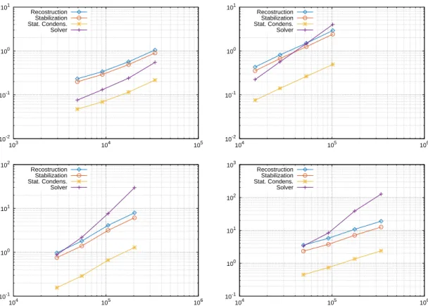
The 3D test cases were run on tetrahedral, hexahedral, and polyhedral meshes obtained from the FVCA6 benchmark set. The tetrahedral meshes have 2003, 3898, 7711 and 15266 elements, the hexahedral meshes have 8, 64, 512 and 4096 elements, and the polyhedral meshes have 1042, 8820 and 28830 elements. In Figures 10, 11, 12, 13 we compare the running time of the various parts of the computation process, in particular the assembly and the global linear system solution. The assembly time scales linearly with the number of degrees of freedom, as expected. In Tables 2 and 3, we summarize the speedups obtained using specialized versus generic data structure on tetrahedral and hexahedral meshes. We observe both in 2D and 3D that assembly times on specialized data structures are significantly lower than assembly times on the generic data structure, confirming that the approach taken in DiSk++ is advantageous. The speedup is particularly welcome in 3D, where the assembly process takes a significant part of the computation time. As a final remark, the solver was not run on the polyhedral meshes because of memory constraints.
10-2 10-1 100 103 104 105 Recostruction Stabilization Stat. Condens. Solver 10-2 10-1 100 101 104 105 106 Recostruction Stabilization Stat. Condens. Solver 10-2 10-1 100 101 102 104 105 106 Recostruction Stabilization Stat. Condens. Solver 10-1 100 101 102 103 104 105 106 Recostruction Stabilization Stat. Condens. Solver
Figure 10: Timings on tetrahedral meshes with respect to DOFs using specialized data structure (from left to right and from top to bottom: k = 0, k = 1, k = 2, k = 3); (violet) crosses: Solver, (red) circles: Stabilization, (blue) diamonds: Reconstruction, (yellow) stars: Static condensation.
10-2 10-1 100 101 103 104 105 Recostruction Stabilization Stat. Condens. Solver 10-2 10-1 100 101 104 105 106 Recostruction Stabilization Stat. Condens. Solver 10-1 100 101 102 104 105 106 Recostruction Stabilization Stat. Condens. Solver 10-1 100 101 102 103 104 105 106 Recostruction Stabilization Stat. Condens. Solver
Figure 11: Timings on tetrahedral meshes with respect to DOFs using generic data structure (from left to right and from top to bottom: k = 0, k = 1, k = 2, k = 3); (violet) crosses: Solver, (red) circles: Stabilization, (blue) diamonds: Reconstruction, (yellow) stars: Static condensation.
DOFs Rec Stab
4912 3.45x 2.44x 9152 2.79x 1.99x 17600 2.77x 1.98x 34009 3.30x 2.34x
DOFs Rec Stab
14736 2.89x 2.66x 27456 2.88x 2.64x 52800 2.54x 2.36x 102027 2.83x 2.58x
DOFs Rec Stab
29472 2.30x 1.97x 54912 2.57x 2.18x 105600 3.08x 2.61x 204054 2.75x 2.33x
DOFs Rec Stab
49120 2.58x 2.11x 91520 2.48x 2.00x 176000 2.71x 2.22x 340090 2.53x 2.08x
Table 2: Speedup in the assembly process (Reconstruction and Stabilization) due to the usage of a special-ized data structure. Tetrahedral meshes, from left to right and from top to bottom: k = 0, k = 1, k = 2, k = 3.
10-5 10-4 10-3 10-2 10-1 100 101 102 103 104 105 Recostruction Stabilization Stat. Condens. Solver 10-4 10-3 10-2 10-1 100 101 102 103 104 105 Recostruction Stabilization Stat. Condens. Solver 10-4 10-3 10-2 10-1 100 101 102 103 104 105 Recostruction Stabilization Stat. Condens. Solver 10-3 10-2 10-1 100 101 102 102 103 104 105 106 Recostruction Stabilization Stat. Condens. Solver
Figure 12: Timings on hexahedral meshes with respect to DOFs using specialized data structure (from left to right and from top to bottom: k = 0, k = 1, k = 2, k = 3); (violet) crosses: Solver, (red) circles: Stabilization, (blue) diamonds: Reconstruction, (yellow) stars: Static condensation.
10-4 10-3 10-2 10-1 100 101 101 102 103 104 105 Recostruction Stabilization Stat. Condens. Solver 10-4 10-3 10-2 10-1 100 101 102 103 104 105 Recostruction Stabilization Stat. Condens. Solver 10-3 10-2 10-1 100 101 102 102 103 104 105 Recostruction Stabilization Stat. Condens. Solver 10-3 10-2 10-1 100 101 102 102 103 104 105 106 Recostruction Stabilization Stat. Condens. Solver
Figure 13: Timings on hexahedral meshes with respect to DOFs using generic data structure (from left to right and from top to bottom: k = 0, k = 1, k = 2, k = 3); (violet) crosses: Solver, (red) circles: Stabilization, (blue) diamonds: Reconstruction, (yellow) stars: Static condensation.
DOFs Rec Stab
60 9.37x 5.09x
336 7.15x 4.98x 2112 8.10x 5.67x 14592 5.98x 4.27x
DOFs Rec Stab
180 3.98x 3.11x 1008 3.08x 2.54x 6336 3.07x 2.66x 43776 3.70x 3.19x
DOFs Rec Stab
360 2.19x 1.94x 2016 3.69x 2.77x 12672 3.22x 2.54x 87552 3.50x 2.77x
DOFs Rec Stab
600 4.19x 3.06x
3360 4.62x 3.43x 21120 3.53x 2.71x 145920 3.35x 2.63x
Table 3: Speedup in the assembly process (Reconstruction and Stabilization) due to the usage of a special-ized data structure. Hexahedral meshes, from left to right and from top to bottom: k = 0, k = 1, k = 2, k = 3.
10-2 10-1 100 101 102 103 104 105 106 Recostruction Stabilization Stat. Condens. 10-1 100 101 102 104 105 106 Recostruction Stabilization Stat. Condens. 10-1 100 101 102 104 105 106 Recostruction Stabilization Stat. Condens. 100 101 102 103 104 105 106 107 Recostruction Stabilization Stat. Condens.
Figure 14: Timings on polyhedral meshes with respect to DOFs using generic data structure (from left to right and from top to bottom: k = 0, k = 1, k = 2, k = 3); (red) circles: Stabilization, (blue) diamonds: Reconstruction, (yellow) stars: Static condensation.