HAL Id: hal-02570967
https://hal.archives-ouvertes.fr/hal-02570967v3
Submitted on 11 Apr 2021
HAL is a multi-disciplinary open access
archive for the deposit and dissemination of
sci-entific research documents, whether they are
pub-lished or not. The documents may come from
teaching and research institutions in France or
abroad, or from public or private research centers.
L’archive ouverte pluridisciplinaire HAL, est
destinée au dépôt et à la diffusion de documents
scientifiques de niveau recherche, publiés ou non,
émanant des établissements d’enseignement et de
recherche français ou étrangers, des laboratoires
publics ou privés.
Disease Clinical Questionnaires
Maxime Peralta, Pierre Jannin, Claire Haegelen, John Baxter
To cite this version:
Maxime Peralta, Pierre Jannin, Claire Haegelen, John Baxter. Data Imputation and Compression For
Parkinson’s Disease Clinical Questionnaires. Artificial Intelligence in Medicine, Elsevier, 2021, 114,
pp.102051. �10.1016/j.artmed.2021.102051�. �hal-02570967v3�
D
C
Q
Maxime Peralta Univ Rennes Inserm, LTSI - UMR 1099
F-35000 Rennes, France
Pierre Jannin Univ Rennes Inserm, LTSI - UMR 1099
F-35000 Rennes, France [email protected]
Claire Haegelen Univ Rennes, CHU Rennes
Inserm, LTSI - UMR 1099 F-35000 Rennes, France
John S.H. Baxter Univ Rennes Inserm, LTSI - UMR 1099
F-35000 Rennes, France [email protected]
April 11, 2021
A
BSTRACTMedical questionnaires are a valuable source of information but are often difficult to analyse due to both their size and the high possibility of having missing values. This is a problematic issue in biomedical data science as it may complicate how individual questionnaire data is represented for statistical or machine learning analysis. In this paper, we propose a deeply-learnt residual autoencoder to simultaneously perform non-linear data imputation and dimensionality reduction. We present an extensive analysis of the dynamics of the performances of this autoencoder regarding the compression rate and the proportion of missing values. This method is evaluated on motor and non-motor clinical questionnaires of the Parkinson’s Progression Markers Initiative (PPMI) database and consistently outperforms linear coupled imputation and reduction approaches.
Keywords Autoencoders · Medical questionnaires · Data imputation · Parkinson’s disease · PPMI
1
Introduction
Data representation is a critical problem in biomedical data science, in which the data available concerning an individual patient can be simultaneously large, uncertain, heterogeneous, and incomplete. It is common knowledge in the machine learning community that accurately curating data and providing a uniform representation are often critical to the success of later approaches. Medical questionnaires are one of the major ways of assessing the clinical state of a patient, providing crucial information necessary to diagnose and monitor patients. Extracting this information is crucial to ensuring patient care in the era of computerised, personalised medicine. Unfortunately, medical questionnaires databases often suffer from missing values for various reasons: some tests cannot be performed by some patients or aren’t performed at each visit, problems can occur when data is computerised, or paper records can be lost. This issue is well known to the research community and addressing it remains an active field of research [1] [2].
Data imputation is an element that addresses this type of heterogeneity by estimating the value of missing elements in an incomplete data vector based on the non-missing elements and the population distribution [3]. Data imputation methods are often employed in research to estimate the value of missing data allowing for downstream analysis or statistical processing to be performed. It has been shown that ignoring data points with missing values not only substantially limits the performance of downstream analysis [4], but also that more accurately imputed data yield
improves performance in downstream analysis [5] [6]. Even simple linear models of retrospective data imputation have been shown in epidemiological and healthcare research to improve the performance of statistical models [7].
A related problem is dimensionality reduction in which a large data vector is reduced into a smaller one that can be more readily analysed to monitor and assess the patient’s situation. Keeping a high dimensional input data vector leads to a problem known in the artificial intelligence community as the ‘curse of dimensionality’ [2]. It has been shown, specifically on electronic health records data, that projecting data into a smaller latent space yield better results than using the original space [8]. The current clinical paradigm is to aggregate related values, summing them into a single score and normalising to account for any missing values. Although simple to implement, this method has been difficult to design [9] with the exact partitioning and summation schemes leading to model misfit and misrepresentation in questionnaires used in Parkinson’s disease [10].
Separately, both data imputation and dimensionality reduction are well-known issues in health informatics recently tackled by machine learning [2], and have both been proven to be beneficial for downstream analysis. Abedia et al. [11] showed that projecting incomplete data to a compressed latent space can be beneficial for data imputation, motivating us to tackle and evaluate these problems altogether. Although compressive autoencoders and deep learning have already been used for data imputation [12], there is, to the best of our knowledge, no paper investigating the dynamics of imputation and reconstruction performance varying the compression amount and the proportion of missing values. Autoencoders are a family of artificial neural networks trained to reproduce its input with a lower dimensional immediate stage or bottleneck [13], which have long been used for data imputation [14]. These networks often consist of a series of encoding layers leading up to a central bottleneck which is then followed by a symmetric series of decoding layers. The central bottleneck creates an “internal representation” of the input data with a lower dimensionality. Autoencoder-based approaches to analysing medical data have been shown to provide useful patient representations for screening broad disease classes [15].
In this paper, we bundle both prospective data imputation and dimensionality reduction into a single method, allowing us to effectively summarise the Parkinson Disease patient’s questionnaire data in a way that can be more readily used for further machine learning methods and population research. We propose a novel autoencoder topology with three novel aspects. First, it uses a custom deep-learnt bias layer in input as an initial imputation strategy. Second, dense layers of the encoder and decoder are organised in a fully-connected fashion. Third, we trained it with a custom, problem-tailored loss function that takes into account the en bloc nature of the missing data of medical questionnaires. For the first time in medical questionnaire imputation, we also investigate the impact of differing levels of compression and differing levels of data corruption on imputation performance, evaluating its response to more realistic forms of missing medical data.
2
Theory and Related Work
2.1 Data Imputation
Imputation can be conceptually split into methods that are applied prospectively, where a possibly complete or incomplete training database is used to estimate missing values for an incomplete and previously unseen data vector, and methods that are applied retrospectively, where information from an incomplete database is extracted in order to estimate its own missing values. In a clinical context, prospective imputation is of greater utility, allowing new patient records to be processed, although retrospective is more commonly used in research contexts in which an entire database is often analysed at the same time.
The most common way of performing retrospective imputation is case deletion, in which every sample with at least one missing value is removed from the database. This method has the benefit of being easy to use, but suffers from two main drawbacks, in addition to not being capable of prospective use. First, if missing values are distributed amongst a large number of samples, it can substantially reduce the size of the database, limiting the power of any statistical or machine learning method. Secondly, if the probability of which values are missing is not independent or changes based on the value the variable would have otherwise taken, removing incomplete lines can introduce bias into the study [16]. Until recently, the most frequently used method for imputation was mean- or median-replacement in which the missing variables are replaced with a constant, specifically the mean or median of the database as a whole [17, 18]. Once a prior database has been collected, it is possible to use this technique prospectively, and it is relatively simple to implement and update as more patients enter the database. However, it is easy to see how this reduces the variability in a database and thus can bias down-stream statistical methods [18].
A common but more nuanced method for data imputation is fitting a linear model to the data. The most commonly used method now is arguably Multiple Imputation through Chained Equations (MICE) in which individual variables
are sequentially imputed in an entire database using simple linear regression, starting with the variable with the least number of missing values and using complete datapoints to initiate the process [19]. The downside of this approach is that it is designed specifically for retrospective use and it is unclear how accurate it would be on unseen data that does not contribute to the construction of the model. Alternatively, Principal Component Analysis (PCA) in particular can be naturally extended to perform prospective imputation by removing the PCA eigenvector components corresponding to the missing values when calculating the PCA scores but using the full eigenvector when transforming the scores back into the data space. Assuming the training database also contains missing values, the PCA decomposition can be determined through several methods [20]. Pairwise correlation PCA (PPCA), for example, computes the mean vector and correlation matrix from all the data vectors available with the corresponding values [20]. Iterative PCA (IPCA) is an expectation-maximisation algorithm that iterates a process of PCA decomposition and imputation until the PCA decomposition converges [21, 22]. These methods are designed to preserve the mean and covariance of the observed data through the process of imputation. The fact that PCA is also a common dimensionality reduction method makes it even more suitable for patient normalisation, although their linear nature may be problematic as aspects of the question may be coupled in a fundamentally non-linear manner. In fact, a recent study of imputation on diabetes clinical questionnaires found the PPCA variant to be more effective than MICE [23] indicating that the heterogeneity in linear methods is indeed meaningful.
Other approaches have taken a similar methodological framework as MICE, but use non-linear rather than linear regression in order to determine the missing values. For example, Random Forest regression in the MICE framework (sometimes referred to as RF-MICE or MICE-RF) does not have a parametric model underlying it. However, in addition to being much more time- and memory-intensive, several recent studies have found the improvement resulting from these non-parametric additions to MICE to be of limited value on clinical data [24, 25].
2.2 Autoencoders
To perform non-linear dimensionality reductionred, inspired by the linear dimensionality reduction of PCA, autoencoders (AE’s) have shown promising results. They have the benefit of capturing more complex or non-linear relations between the inputs. Stacked denoising AE’s [26] are particularly useful as they have highly robust denoising capabilities resulting from having noise (theoretically of the same distribution as would be observed in the testing phase) injected into their input during training.
AE’s can also be designed with large-scale data imputation explicitly in mind. For example, correlation neural networks[27] attempt to find correlated, modality independent internal representations from missing modality problems, where large portions of the data vector are missing simultaneously. Unfortunately, the regularisation term which encourages this correlation requires a low number of modalities and complete data vectors for training which limits their applicability to medical questionnaires where this may not be the case.
Nevertheless, neural networks can be difficult to design and to train for various reasons. Primarily, the shape of the neural network highly affects its performance. For example, even assuming low parameterisation and risk of overfitting, a shallow neural network may not be able to capture the non-linearities of the inputs, while a too deep neural network could suffer from training issues such as inability to propagate gradients effectively.
In this paper, we propose a method relying on an autoencoder architecture with a densely-connected encoder and decoder consisting of fully-connected layers, which we call a Fully Connected Autoencoder (FCAE), to address both data imputation and dimensionality reduction.
3
Materials and Methods
The input data is first rescaled in the range [0,1], with min-max scaling based on the highest and lowest values possible for each question. Although this does not necessarily reflect the semantic meaning behind different levels in the ordinal variables, it does ensure that the number of levels in each does not excessively bias the training of the network and is commonly used even for ordinal data [28]. Denoising autoencoders are then constructed with masking noise applied to the input layer in order to simulate missing values. Unlike truly missing values, their reconstruction quality can still appear in the loss function. This is implemented through a custom masking layer which randomly removes an entire modality (collection of inputs taken from the same test and thus tend to be missing or be present en bloc).
The input to the encoder consists of both the data and a mask which indicates the presence of missing data. The encoder consists of the bias layer, which chooses particular initial values to assign to missing variables as a form of initial naive imputation, followed by a series of dense layers, the output of which is concatenated to the input for the successive layers, as shown in Figure 1(a). This alternation between dense and concatenation layers is motivated in a similar way as residual networks [29] in that they allow for short-cuts, minimising issues with propagating gradients while allowing
Dropout
Dense
Activation
Concatenate
Input
Output
(a) Computational Block
Bias(281)
Input(281)
CompBlock(291)
CompBlock(301)
CompBlock(311)
CompBlock(321)
CompBlock(331)
CompBlock(341)
CompBlock(351)
Dense(3)
IR(3)
(b) EncoderDense(281)
IR(3)
CompBlock(13)
CompBlock(23)
CompBlock(33)
CompBlock(43)
CompBlock(53)
CompBlock(63)
CompBlock(73)
Output(281)
(c) DecoderFigure 1: Structure of the FCAE, relying on the chaining of a residual substructure called “Computational Block”, presented in (a). The input is passed through the encoder, which produces the internal representation, as shown in (b). The decoder tries to reconstruct/impute the input from this internal representation, as shown in (c). The size of the output of each block is shown in parenthesis. In the given example, the internal representation (IR) size is equal to 3.
for higher depths to be used to capture non-linearities, and has already been used successfully for data imputation [30]. The final layer of the encoder is a dense layer used to estimate the internal representation. The decoder is constructed similarly to the encoder, with a series of computational blocks each receiving the internal representation and the output of all previous decoder layers as input. Each dense layer is composed of 10 neurons and both the encoder and decoder have a depth of 7 layers, leading to an overall depth of 15. Dropout (5%) was applied to the input of each layer except the final one. Rectified Linear Units (ReLU) were used as the activation functions for each dense layer. The proposed structure (shown in Figure 1) is similar to that of multimodal autoencoders [31] with the exception of our concatenation structure and that the noise operator is performed within the network as a layer rather than used to augment the dataset prior to training.
In order to improve the convergence of the autoencoder during training and to minimize the effects of random weight initialisation, each FCAE began with an initialisation step. The bias layer was initialised to replace missing values with the mean value of the respective variable. Each encoder layer was then greedily initialised to the PCA transform that preserved the largest amount of information from its input. Each decoder layer was initialised with linear regression to create the optimal reconstruction given the input to that particular output layer. This initialization guarantees that the training set performance of the FCAE is at worst equivalent to that of the pairwise PCA variant. This step was performed using the entirety of the training dataset simultaneously, but did not involve data augmentation.
The hyperparameters for the network were determined in a two-step process. First, we defined the topology of the network using a grid search, in order to optimize the number of neurons per dense layer and the depth of the network while keeping the other parameters at a constant value. Second, we optimized training-related parameters (keeping the network structure fixed), such as learning rate, batch size and dropout rate, in a Bayesian manner using a Gaussian processes as a surrogate model and expected improvement as the criterion.
The networks were implemented in Keras using a TensorFlow back-end with NAdam as the optimizer. We have made available the code to build and compile our proposed autoencoder, at https://github.com/m-prl/PatiNAE.
0 2000 4000 6000 0 500 1000 1500 100 200
Number of Missing Values
Number of Ro ws (cum ulativ e) Number of Ro ws
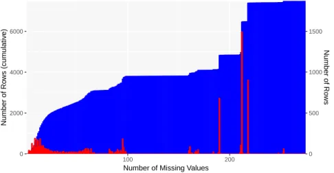
Figure 2: Histogram of PPMI questionnaire data by number of missing values. The cumulative histogram is shown in blue (left axis) and the frequency in red (right axis).The number of rows is shown, indicating the number of questionnaires with a particular quantity of missing data.
3.1 Accuracy, Loss and Regularisation Metrics
For the purpose of evaluating each compressing data imputation approach, two measures of accuracy based on the input, x, and reconstruction values, ˆx, were used:
A1= 1 K N X i=1 M X i=j
(ˆx(i)j − x(i)j )2∗ Mj(i) (1)
A2= 1 U N X i=1 M X j=1
(ˆx(i)j − x(i)j )2∗ (1 − Mj(i)) (2)
where K is the number of known values and U the number of unknown values in the dataset being evaluated, and Mj(i) is a mask identifying the known values. For A2, additional unknown values must be inserted into the dataset in order
for their ground-truth value (x(i)j ) to be known for evaluation purposes.
For training, the loss metric, analog to the one used by Sanchez et al. [5], used a weighted mean squared reconstruction error using both a binary mask to identify missing data (Mmiss) and a second binary mask to identify data that has been
dropped in the process of data augmentation (Mdrop):
L = 1 K + U N X i=1 M X i=j
(ˆx(i)j − x(i)j )2∗ (1 − Mmiss,j(i) )
+ 4 ∗
M
X
i=j
(ˆx(i)j − x(i)j )2∗ Mdrop,j(i)
(3)
The weighting factor of is equivalent to put a higher importance into reconstructing the dropped data and thus preferentially improves the network’s A2accuracy. A weighting factor of 4 showed the most interesting results.
3.2 PPMI Questionnaire Database
The Parkinson’s Progression Markers Initiative (PPMI) [32] is a program sponsored by the Michael J. Fox Foundation for Parkinson’s Research. It is an observational clinical study which tracks cohorts of subjects with different forms of Parkinson’s disease for up to 8 years with the goal of identifying biomarkers of disease progression using MR imaging, biologic sampling as well as clinical and behavioural assessments.
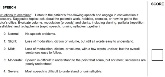
Figure 3: First question of Part 3 (motor examination) of the MDS-UPDRS test (version as of May 2, 2019).
Questionnaire % comp. % incomp. % mod. miss. miss. rate
UPDRS I 98.84 0.03 1.13 16.67 UPDRS I PQ 98.80 0.04 1.16 23.81 UPDRS II 96.52 2.43 1.05 10.99 UPDRS III 2 94.73 3.27 6.51 UPDRS IV 55.91 0.04 44.05 61.11 S&E 98.79 0 1.21 N/A PASE 13.72 15.41 70.87 22.12 SCOPA AUT 0 50.89 49.11 9.37 MCI 38.65 0 61.35 N/A Ger. Dep. 50.68 0.17 49.15 9.23 QUIP 32.03 18.85 49.12 15.04 STA Inv. 50.43 0.41 49.16 9.27
Benton JLO 40.60 0 59.40 N/A
Hopkins VLT 40.76 0.81 58.42 39.47
L-N Seq. PD 4.15 37.25 58.60 30.60
MoCA 46.33 0.12 53.55 13.10
Sem. Flu. 41.54 0 58.46 N/A
Symb. Dig. Mod. 41.44 0.07 58.49 50.00
Epworth sleep. 50.80 0.04 49.16 12.50
REM SD Quest. 54.07 0.65 45.27 6.32
Average 47.80 11.10 41.10 21.01
Table 1: Statistics of PPMI questionnaires regarding missing values. The second, third and fourth columns show the percentage of rows being complete, with missing values, and with the entire modality missing, respectively. The last row shows the mean percentage of missing values for the incomplete rows.
This work is focused on the clinical and behavioural assessments which were designed to provide a satisfactory amount of information regarding the patient’s motor, cognitive, neuro-behavioural and neuro-psychological state. The database was built collecting and merging data from most of the motor and non-motor tests. The tests presented on the database are: MDS-UPDRS (all parts), Physical Activity Scale for the Elderly - Household Activity, Modified Schwab & England ADL, SCOPA-AUT, Clinical Cognitive Categorisation, Geriatric Depression Scale (Short), Questionnaire for Impulsive-Compulsive Disorders (QUIP), State-Trait Anxiety Inventory, Benton Judgement of Line Orientation, Hopkins Verbal Learning Test, Letter-Number Sequencing (PD), Montreal Cognitive Assessment (MoCA), Semantic Fluency, Symbol Digit Modalities Text, Epworth Sleepiness Scale, Features of REM Behaviour Disorder. Some parts were discarded because they where performed too sparsely (on too few patients or just at one visit). We built our database by pooling the tests of each cohorts at each visit, on April 2018. The constructed PPMI database has 281 columns and 7490 rows across 1011 patients. 42.9% of the data is missing in a highly heterogeneous manner. The questions used in these tests mostly permit ordinal answers. These tests do not include questions that permit categorical answers, but there are a few that permit continuous-valued ones. Figure 3 shows the first item of part 3 of the MDS-UPDRS test, which is a question with an ordinal answer. Table 1 gives statistics regarding missing values and modalities for each questionnaire used in this study. The names of the questionnaires have been shorten for clarity purpose, and are in the same order than presented in this section. This table shows a great heterogenity in the way that values are missing. Nonetheless, the major cause of missing values is when the whole modality is missing en bloc. Note that the large majority of missing values are due to the protocol design, as not all tests are performed, nor are intended to be performed, at each visit for each cohort. This is well described in the PPMI database’s protocol information. An extensive study on the MDS-UPDRS questionnaire (present in the PPMI database) as been performed by Goetz et. al. [33], showing that the loss of information is consequential even with only a few missing values. In their analysis, removing 0-27% of answers completely at random drastically reduces the coherence of the remaining answers. This scenario is obviously worsened by the removal of entire modalities, rather than individual questions, a not uncommon occurrence as shown in Table 1. This shows the quasi-independent nature of the questions of medical questionnaires, even between different items of a same test.
3.3 Comparative Approaches
We compared our results with three comparative approaches. The most simple is mean imputation, in which each missing value is replaced with the mean of the corresponding variable. This is the most accurate solution when no internal representation (i.e. no information about the available data) is allowed to be used in the reconstruction process. Pairwise correlation principle component analysis (PPCA) [20] and iterative principle component analysis (IPCA) [21] are the two others comparative approaches. As stated in Section 2.1, they are common PCA-based approaches to dimensionality reduction simultaneous with data imputation.
4
Experiments
We have three hypotheses to experimentally verify:
• H1: there is an optimal internal representation (IR) size to minimise error. That is, there is a degree of flexibility in terms of the networks’ performance that diminishes the network’s A2performance. This is expected for
PCA in which, after a certain point, additional variables allows the IR to “remember” missing values as the mean of their corresponding variable rather than impute them.
• H2: the network reconstructs data vectors more accurately when they are more complete, decreasing in performance as data becomes missing.
• H3: there is a benefit from learning from incomplete data points. Although complete data vectors are unarguably better, using case deletion to restrict the training dataset to only those data points reduces performance. All p-values shown are post Bonferroni correction to account for multiple tests. All tests performed are paired t-tests. Prior to the experiments, all the data is normalized to the [0, 1] range using each variable’s theoretical maximum and minimum values. This equally weights variables regardless of discrepancies in their range.
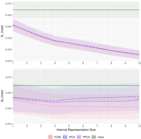
H1: Optimal IR Size
This experiment consists of training and testing autoencoders (and comparative PCA approaches) with IR sizes ranging from 1 to 10. In order to handle the low number of data-points, 20-fold cross-validation was performed to estimate the error. After splitting the dataset into 20 folds, one fold was iteratively selected as the testing dataset. The testing dataset was randomly corrupted with 10% chance of a modality being removed. This corruption process was repeated
0.045 0.050 0.055 0.060 0.065 0.070 1 2 3 4 5 6 7 8 9 10 A1 (mse) 0.055 0.060 0.065 0.070 1 2 3 4 5 6 7 8 9 10
Internal Representation Size
A2
(mse)
Method FCAE IPCA PPCA mean
Figure 4: A1(top) and A2(bottom) error for data reconstruction using FCAE (red) and comparative IPCA (blue) and
PPCA (purple) under varying IR size. The solid green line is the performance of mean data imputation with the dotted green lines representing the standard deviation thereof.
40 times in order to have 40 differently corrupted versions of each testing dataset and total number of 800 datapoints for comparison. The datasets were saved to ensure that the same ones were used for evaluating each method, allowing for paired tests.
The remaining 19 folds were again split at each iteration with 80% as training data and 20% as validation data. The FCAE were re-initialised and retrained 8 times per iteration, and the one receiving the lowest validation A2error was
selected to be evaluated on the testing dataset.
Dataset splitting was performed patient-wise, assigning all of the data from a patient into the same fold, implying that clinical records for one patient at two different times could not appear in both training and testing simultaneously. The validation dataset is corrupted in the same manner as the testing dataset to ensure that the validation loss represents both A1and A2testing error.
The A1and A2errors are shown in Figure 4. As expected, the A1error decreased monotonically with IR size for all
methods (p < 0.01). As hypothesised, A2did show an optimal IR size for the PCA approaches with both methods
monotonically decreasing until IR = 4 (p < 0.01) and monotonically increasing afterwards (p < 0.01 with the exception of PPCA between IR = 7 & 8). For FCAE, however, this consistent monotonic increase did not appear indicating that the learning process encouraged the AE to more actively impute that data. Our FCAE also performed better (p < 0.01) than both PCA-based methods for both A1 and A2 at all IR sizes indicating that there is some
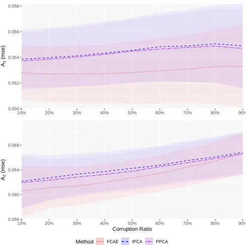
non-linearity in the underlying structure of the data. H2: Predicting with Missing Data
This experiment was performed by training each method on all the available data and verifying that the testing error increases with an increasing corruption ratio. The methods were assigned an IR size of 4, corresponding to the optimal
0.050 0.052 0.054 0.056 0.058 10% 20% 30% 40% 50% 60% 70% 80% 90% A1 (mse) 0.056 0.060 0.064 0.068 10% 20% 30% 40% 50% 60% 70% 80% 90% Corruption Ratio A2 (mse)
Method FCAE IPCA PPCA
Figure 5: A1(top) and A2(bottom) error for data reconstruction using FCAE (red) and comparative IPCA (blue) and
PPCA (purple) under varying levels of corruption.
size determined in Section 4. The FCAE was trained with a corruption ratio of 10%, matching the lowest level of corruption performed. The results of this experiment are shown in Figure 5. As expected, the performance of all methods degraded for A2as the corruption ratio increased (p < 0.01 between each consecutive corruption ratio, for
every method), reflecting the decreasing amount of information available to the network to use in reconstruction. For A1, the degradation is subtler, especially for the FCAE which does not show a significant change in performance
between 10% and 40% corruption rates.
The FCAE method outperformed both PCA approaches for both metrics at every corruption level (p < 0.01). FCAE seem to be more sensitive to the amount of data missing compared to PCA, which may be the result of the discrepancy between the corruption ratio used during training and the one used in evaluation, significantly changing the training and testing distributions.
H3: Learning from Incomplete Data
This experiment consisted in training and testing FCAE and comparative PCA approaches, with IR size of 4, by discarding training and validation data samples that presents more than a fixed percentage of variables missing (which we will call the discard threshold). No testing data was removed. This was done in a cross-validation style similar to Section 4. The A1and A2results are shown in Figure 6.
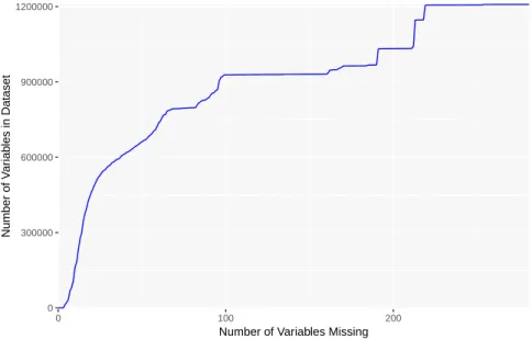
Generally speaking, each method performed slightly better as more (although more incomplete) training data was provided. For all approaches, the improvement was very modest between consecutive discard thresholds with the exception of 10% and 20%. As shown in Figure 7, this is likely due to the larger number of added rows between those discard thresholds, compared to later thresholds. (As with the cumulative information in Figure 2, Figure 7 is an indication of the amount of data available, although in terms of the sheer volume of data rather than number of datapoints. That is, datapoints with half their values missing have half the volume of complete datapoints, reflected in
0.050 0.052 0.054 0.056 10% 20% 30% 40% 50% 60% 70% 80% 90% A1 (mse) 0.0550 0.0575 0.0600 0.0625 0.0650 0.0675 10% 20% 30% 40% 50% 60% 70% 80% 90% Discard Threshold A2 (mse)
Method FCAE IPCA PPCA
Figure 6: A1(top) and A2(bottom) error for FCAE (red) and comparative IPCA (blue) and PPCA (purple) methods
with varying toss ratios.
0 300000 600000 900000 1200000 0 100 200
Number of Variables Missing
Number of V
ar
iab
les in Dataset
Figure 7: Number of variables available when all rows with more than a certain number of missing variables (x-axis) are removed.
Method Comp. time (µs) Uncomp time (µs)
PPCA 1.14 1.16
IPCA 1.05 1.27
FCAE 33.9 26.1
Table 2: Average per sample compression and decompression time for our proposed autoencoder and the two baselines, with an Intel Xeon E5-1620 v4 CPU at 3.50GHz. All values are expressed in microseconds.
this figure, but are given equal weight in Figure 2.) There was another swift increase between 60% and 80%, which can be seen in the improvements in the FCAE’s A1and A2errors. This provides some evidence that training with
incomplete data is beneficial, even if a sizeable portion of the dataset is largely incomplete.
It is interesting to note that the FCAE initially performed statistically significantly worse for A1than the comparative
PCA approaches at the lowest discard thresholds (10% and 20%, p < 0.01), but significantly better at higher ones (70% to 90%, p < 0.01). This is likely because of the greater flexibility of the model, having more degrees-of-freedom and thus requiring more data to successfully fit.
4.1 Computation time
In order to quantify the computation time required for our method and the baselines, we ran a 20-fold cross-validation and measured the time required to compress and to uncompress the testing set. The results, in microsecond per sample, are displayed in Table 2, using an Intel Xeon E5-1620 v4 CPU at 3.50GHz.
Although our proposed autoencoder requires about 30 times more time to compress and uncompress a data sample, this would not be significant in a clinical setting as each method can be easily considered real-time.
5
Discussion and Future Work
We compared our method to two state-of-the-art versions of PCA. To the best of our knowledge, PCA is the only commonly-used method that combines both imputation and compression and provides some optimality guarantees as a linear baseline. The first point of discussion is the relatively good performance of the two variants of PCA, indicating that a large amount of the variation can be addressed by a linear model equipped with simple missing-value handling. The difference between the two approaches to constructing linear models (PPCA and IPCA) was smaller than initially expected, with the more complex IPCA underperforming PPCA, illustrating that the linear approximation of the dataset’s underlying structure is only that: an approximation.
The issue with using these linear models for reconstruction was expected: a sufficiently large internal representation allows PCA to “remember” the missing variables as their mean value rather than impute them. The deterioration of A2
after a certain point in PCA is visible even at the relatively low IR sizes shown in Figure 4 (bottom). This trade-off is much less pronounced in the FCAE likely due to the application of modality masking noise which implies that the loss metric encodes both A1 and A2. This combination of losses means that the FCAE must take a more complex
imputation strategy even at higher IR sizes.
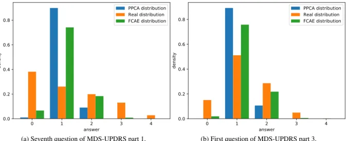
We observed the distribution of the output prediction of each item, as seen in Figure 8. In this figure, we compare the output distribution of the first question of the part 3 (motor examination) of the MDS-UPDRS questionnaire as reconstructed using FCAE and PPCA on a test set against the true distribution as recorded in the database. 40 iterations have been performed, with a corruption ratio of 10% and IR size of 4. We can notice that there is an important loss of variance in the distributions, especially with PPCA reconstruction. We can explain that by the reconstruction algorithms being designed to minimize a variant of the mean squared error, thus biasing predictions values towards the mean of the distribution and penalising extrema. This behaviour is seen in both reconstruction methods although less distinctly in FCAE indicating that it has a higher capability of reconstructing these extreme values. We have found that this reduction in variance is common across all questions in the database, possibly due to the inherent uncertainty and subjectivity of the variables encouraging some regression-towards-the-mean.
In addition, the variables investigated in Figure 8 show two distinct underlying distributes, with the first question of UPDRS part 3 having something similar to a binomial distribution with the seventh question of UPDRS part 1 having something closer to a geometric distribution. Unsurprisingly, the linear baseline’s reconstruction for both is more binomial-shaped, given that binomial distributions are more similar to discretely-sampled Gaussian distributions, the continuous version being explicitly optimized for by linear methods. Perhaps unsurprisingly, the proposed auto-encoder method shows a similar tendency, which indicates that the likely cause is the L2-style loss function similar to it and
0 1 2 3 4 answer 0.0 0.2 0.4 0.6 0.8 density PPCA distribution Real distribution FCAE distribution
(a) Seventh question of MDS-UPDRS part 1.
0 1 2 3 4 answer 0.0 0.2 0.4 0.6 0.8 density PPCA distribution Real distribution FCAE distribution
(b) First question of MDS-UPDRS part 3.
Figure 8: True distribution compared with output distribution of FCAE and PPCA for two questions from the MDS-UPDRS test.
the baseline methods. One possible expansion for the auto-encoder framework is the design of a heterogeneous loss function that is more cognisant of these distributional differences rather than the use of an equivalent L2 loss across all the questions in the database regardless of their distributional characteristics. These distributional differences would also play an important role in evaluating any imputation method, especially model-based methods such as MICE [19], as it implies that the L2 loss is not a representative metric for error. MICE in particular is versatile with respect to this as each variable is imputed individually and thus individual attention can be given to its error model [19]. Despite this capability, Hong et al. [34] have still found MICE (as well as Random Forest Imputation, a similar non-linear method) to still experience a similar bias in the case of highly non-normal or skewed data. In addition, from a data leakage perspective important to consider when prospective use is envisioned, this attention would have to be treated with caution as the type of distribution of the ground-truth data would have to be inferred from datapoints that are not used in any testing set. Given that cross-validation was used to account for limited data, isolating a sufficiently large portion of the training data to adequately infer the distribution’s family and estimated parameterization could be problematic. In future, we would like to extend our analysis of medical questionnaire imputation and compression for a particular downstream analysis goal, such as the classification of different Parkinsonian patient groups or the stratification of the disorder. At the moment, diagnosis and stratification are done by a neurologist using some of the data provided by the medical questionnaire, indicating the utility of making the analysis thereof more objective and robust to heterogeneous, incomplete data.
One fact that complicates this study is the relatively low number of data points, especially complete data points, given the relatively high dimensionality and lack of simplifying structure in each point. These issues are further complicated by the majority of tests in the PPMI database used having a middling number of ordinal values (most variables took on values in {0..5}) rather than simpler categorical or continuous values which thus limit their utility as input.
Ordinal and categorical data handling
It is important to note that, with this database, all the variables were numerical or ordinal. Thus, we did not test the framework with categorical variables, which can be present in other medical questionnaires. We would suggest the use of one-hot encoding for this type of variable in addition to a custom output layer capable of handling different loss functions for the different variable types.
Imputing ordinal variables is problematic. Although ordered, the leap between two successive categories is not consistent, nor quantified. Thus, an error in imputation for an ordinal variable can be more or less significant in certain parts of the answers range. In medical questionnaires, some questions suffer greatly from this problem, as a ’0’ could mean complete absence of a symptom, and ’1’ to ’4’ could quantify its severity. To this extent, the difference between ’0’ and ’1’ has more impact on clinical interpretation than the difference between ’1’ and ’2’. Neither our method, nor the baselines, straightforwardly address the specificities of ordinal variables, but instead treat them as continuous, a common approach in the literature [28]. One way of tackling this problem with our framework would be to use a loss function tailored for ordinal variables, such as the weighted kappa loss proposed by De la Torre et al. [35]. Ideally, the
weights of each consecutive error of each ordinal variable should be defined by clinicians according to its impact on clinical interpretation, thus leading to a greater practical applicability.
An alternative approach would be to use an adversarial loss that could, in theory, learn what continuous values correspond with possible levels for each ordinary variable and well as what combination of values are realistic [6]. Such an approach would require a significant database consisting of full rows, i.e. data that can be used as true fully sampled data for training the discriminator. However, this is not representative of the PPMI database as described in Section 3.2.
6
Conclusions
This paper presents an autoencoder specifically designed for data imputation and compression of medical questionnaires, in which entire modalities may be missing. This represents some of the initial steps into performing deep learning on specific medical tasks that are challenging due to the dataset size compared to the high number of features, the data types provided and the complexity of the learning problem. We have shown that significant and consistent improvements can be made over linear methods, especially when a lower number of features is missing. We have also shown that their is an interest in learning on incomplete data vector, and that the imputation performance of our framework is not negatively impacted by a high internal representation size, making the downstream choice of the compression rate easier.
Acknowledgments
Maxime Peralta’s PhD is funded by the Fondation pour la Recherche Médicale (FRM). John Baxter is supported by a Post-Doctoral Fellowship from the Natural Sciences and Research Council of Canada (NSERC) and by the Institut des Neurosciences Cliniques de Rennes (INCR).
Data used in the preparation of this article were obtained from the Parkinson’s Progression Markers Initiative (PPMI) database (www.ppmi-info.org/data). For up-to-date information on the study, visit www.ppmi-info.org. PPMI - a public-private partnership - is funded by the Michael J. Fox Foundation for Parkinson’s Research and funding partners, including AbbVie, Allergan, Avid Radiopharmaceuticals, Biogen, BioLegend, Bristol-Myers Squibb, Celgene, Denali Therapeutics, GE Healthcare, Genentech, GlaxoSmithKline, Lilly, Lundbeck, Merck, Meso Scale Discovery, Pfizer, Piramal, Prevail, Roche, Sanofi-Genzyme, Servier, Takeda, Teva, UCB, Verily, Voyager Therapeutics and Golub Capital.
References
[1] Brett K Beaulieu-Jones, Daniel R Lavage, John W Snyder, Jason H Moore, Sarah A Pendergrass, and Christopher R Bauer. Characterizing and managing missing structured data in electronic health records: data analysis. JMIR medical informatics, 6(1):e11, 2018.
[2] Siddharth Srivastava, Sumit Soman, Astha Rai, and Praveen K Srivastava. Deep learning for health informatics: Recent trends and future directions. In 2017 International Conference on Advances in Computing, Communications and Informatics (ICACCI), pages 1665–1670. IEEE, 2017.
[3] Bradley Efron. Missing data, imputation, and the bootstrap. Journal of the American Statistical Association, 89(426):463–475, 1994.
[4] Swagatam Das, Shounak Datta, and Bidyut B Chaudhuri. Handling data irregularities in classification: Foundations, trends, and future challenges. Pattern Recognition, 81:674–693, 2018.
[5] Adrián Sánchez-Morales, José-Luis Sancho-Gómez, Juan-Antonio Martínez-García, and Aníbal R Figueiras-Vidal. Improving deep learning performance with missing values via deletion and compensation. Neural Computing and Applications, pages 1–12, 2019.
[6] Uiwon Hwang, Sungwoon Choi, Han-Byoel Lee, and Sungroh Yoon. Adversarial training for disease prediction from electronic health records with missing data. arXiv preprint arXiv:1711.04126, 2017.
[7] Karel GM Moons, Rogier ART Donders, Theo Stijnen, and Frank E Harrell Jr. Using the outcome for imputation of missing predictor values was preferred. Journal of clinical epidemiology, 59(10):1092–1101, 2006.
[8] Cao Xiao, Edward Choi, and Jimeng Sun. Opportunities and challenges in developing deep learning models using electronic health records data: a systematic review. Journal of the American Medical Informatics Association, 25(10):1419–1428, 2018.
[9] Joseph M Kishton and Keith F Widaman. Unidimensional versus domain representative parceling of questionnaire items: An empirical example. Educational and Psychological Measurement, 54(3):757–765, 1994.
[10] Peter Hagell and Maria H Nilsson. The 39-item parkinson’s disease questionnaire (pdq-39): is it a unidimensional construct? Therapeutic Advances in Neurological Disorders, 2(4):205–214, 2009.
[11] Vida Abedi, Manu K Shivakumar, Pinyi Lu, Raquel Hontecillas, Andrew Leber, Monika Ahuja, Alvaro E Ulloa, Joshua M Shellenberger, and Josep Bassaganya-Riera. Latent-based imputation of laboratory measures from electronic health records: Case for complex diseases. bioRxiv, page 275743, 2018.
[12] Brett K Beaulieu-Jones and Jason H Moore. Missing data imputation in the electronic health record using deeply learned autoencoders. In Pacific Symposium on Biocomputing 2017, pages 207–218. World Scientific, 2017. [13] Geoffrey E Hinton and Ruslan R Salakhutdinov. Reducing the dimensionality of data with neural networks.
science, 313(5786):504–507, 2006.
[14] Mussa Abdella and Tshilidzi Marwala. The use of genetic algorithms and neural networks to approximate missing data in database. In Computational Cybernetics, 2005. ICCC 2005. IEEE 3rd International Conference on, pages 207–212. IEEE, 2005.
[15] Riccardo Miotto, Li Li, Brian A Kidd, and Joel T Dudley. Deep patient: an unsupervised representation to predict the future of patients from the electronic health records. Scientific reports, 6:26094, 2016.
[16] Paul D Allison. Missing data. Sage publications, 2001.
[17] Xiao-Hua Zhou, George J Eckert, and William M Tierney. Multiple imputation in public health research. Statistics in medicine, 20(9-10):1541–1549, 2001.
[18] A Rogier T Donders, Geert JMG Van Der Heijden, Theo Stijnen, and Karel GM Moons. A gentle introduction to imputation of missing values. Journal of clinical epidemiology, 59(10):1087–1091, 2006.
[19] Ian R White, Patrick Royston, and Angela M Wood. Multiple imputation using chained equations: issues and guidance for practice. Statistics in medicine, 30(4):377–399, 2011.
[20] Stéphane Dray and Julie Josse. Principal component analysis with missing values: a comparative survey of methods. Plant Ecology, 216(5):657–667, 2015.
[21] Henk AL Kiers. Weighted least squares fitting using ordinary least squares algorithms. Psychometrika, 62(2):251– 266, 1997.
[22] Julie Josse, François Husson, and Jérôme Pagès. Gestion des données manquantes en analyse en composantes principales. Journal de la Société Française de Statistique, 150(2):28–51, 2009.
[23] Harshad Hegde, Neel Shimpi, Aloksagar Panny, Ingrid Glurich, Pamela Christie, and Amit Acharya. Mice vs ppca: missing data imputation in healthcare. Informatics in Medicine Unlocked, 17:100275, 2019.
[24] Emily Slade and Melissa G Naylor. A fair comparison of tree-based and parametric methods in multiple imputation by chained equations. Statistics in medicine, 39(8):1156–1166, 2020.
[25] Burim Ramosaj, Lubna Amro, and Markus Pauly. A cautionary tale on using imputation methods for inference in matched-pairs design. Bioinformatics, 36(10):3099–3106, 2020.
[26] Pascal Vincent, Hugo Larochelle, Isabelle Lajoie, Yoshua Bengio, and Pierre-Antoine Manzagol. Stacked denoising autoencoders: Learning useful representations in a deep network with a local denoising criterion. Journal of Machine Learning Research, 11(Dec):3371–3408, 2010.
[27] Sarath Chandar, Mitesh M Khapra, Hugo Larochelle, and Balaraman Ravindran. Correlational neural networks. Neural computation, 28(2):257–285, 2016.
[28] Hongbao Zhang, Pengtao Xie, and Eric Xing. Missing value imputation based on deep generative models. arXiv preprint arXiv:1808.01684, 2018.
[29] Gao Huang, Zhuang Liu, Laurens Van Der Maaten, and Kilian Q Weinberger. Densely connected convolutional networks. In Proceedings of the IEEE conference on computer vision and pattern recognition, pages 4700–4708, 2017.
[30] Adriana Fonseca Costa, Miriam Seoane Santos, Jastin Pompeu Soares, and Pedro Henriques Abreu. Missing data imputation via denoising autoencoders: the untold story. In International Symposium on Intelligent Data Analysis, pages 87–98. Springer, 2018.
[31] Natasha Jaques, Sara Taylor, Akane Sano, and Rosalind Picard. Multimodal autoencoder: A deep learning approach to filling in missing sensor data and enabling better mood prediction. In Proc. International Conference on Affective Computing and Intelligent Interaction (ACII), San Antonio, Texas, 2017.
[32] Kenneth Marek, Danna Jennings, Shirley Lasch, Andrew Siderowf, Caroline Tanner, Tanya Simuni, Chris Coffey, Karl Kieburtz, Emily Flagg, Sohini Chowdhury, et al. The parkinson progression marker initiative (ppmi). Progress in neurobiology, 95(4):629–635, 2011.
[33] Christopher G Goetz, Sheng Luo, Lu Wang, Barbara C Tilley, Nancy R LaPelle, and Glenn T Stebbins. Handling missing values in the mds-updrs. Movement Disorders, 30(12):1632–1638, 2015.
[34] Shangzhi Hong and Henry S Lynn. Accuracy of random-forest-based imputation of missing data in the presence of non-normality, non-linearity, and interaction. BMC medical research methodology, 20(1):1–12, 2020. [35] Jordi de La Torre, Domenec Puig, and Aida Valls. Weighted kappa loss function for multi-class classification of