Using Active Networking for Congestion Control in High-speed
Networks with Self-similar Traffic
Tibor Gyires
Illinois State University
tbgyires@ilstu.edu
Abstract
Various papers discuss the impact of burstiness on network congestion. Their conclusions are that congested periods can be quite long with packet losses that are heavily concentrated. Several conventional methods have been implemented to avoid congestion, such as traffic shaping, end-to-end feedback congestion control systems, etc. These methods are not responsive enough to the varying bandwidth and network delay caused by bursty traffic. The objective of our paper is to describe a new algorithm to avoid congestion without the negative effects of the traditional methods. A model developed under Compuware’s COMNET the discrete event simulation system, illustrates the algorithm. The model is based on real traffic collected in an ATM network.
1. Introduction
Measurements of real traffic indicate that burstiness is present on a wide range of time scales [ 1,2,3,4]. Traffic that
is bursty on many or all time scales can be described statistically using the notion of self-similarity. In bursty traffic the term self-similarity is used in a distribution sense: when viewed at varying scales, the traffic’s distribution remains unchanged. Various papers [ 1,3,4,5,6] discuss the impact of the burstiness on network congestion. Their conclusions are that
0 congested periods can be quite long with packet losses
that are heavily concentrated,
0 linear increases in buffer size do not result in large
decreases in packet drop rates, and
0 a slight increase in the number of active connections
can result in a large increase in the packet loss rate.
Results show that packet traffic “spikes” (which cause actual losses) ride on longer-term “ripples”, that in turn ride on still longer-term “swells” [l].
Several conventional methods have been implemented to avoid congestion, such as traffic shaping, end-to-end feedback congestion control systems, etc. Traffic shaping, spreading the packets in time, introduces an unacceptable
delay when the traffic is generated at high-speed in long
bursts. Feedback based congestion control systems are not responsive enough to the varying bandwidth and network delay. The larger the end-to-end delay, the longer it takes to inform the sending nodes that the network has become congested. It was shown in [7], that the duration of the congestion at the congested routers is directly related to the bandwidth-delay product.
A new research direction, active networking, offers a more promising solution for congestion control. Active networks allow designers to program the network software and hardware to manipulate the network’s behavior. For instance, the ACC project recommends an active network solution to reduce the delay when congestion is signaled to the sending node [8]. ACC packets are sent containing the congestion window size that the sender adjusts. When congestion occurs at a router, it determines the congestion window size, drops packets that would not be sent with the new window size, and notifies the sender about the new window size. ACC extends the congestion control points from the endpoints into the active nodes where they can immediately react to congestion. The downstream nodes see traffic that looks as if the sender had reacted immediately.
We propose a new active network algorithm that can reduce the harmful consequences of congestion due to aggregated bursty traffic. Many methods for measuring traffic burstiness are based on the estimate of the Hurst parameter in addition to the bursts’ mean and variance. The Hurst parameter 0.5 < Hurts < 1 is a measurement in fractal geometry to characterize self-similarity of objects. The higher the value of Hurst, the higher the burstiness, and consequently the worse the queuing performance of switches and routers along the traffic path [3]. The frst
packet of a connection and subsequent control packets carry the anticipated traffic’s Hurst parameter. It is calculated from previous connections and applications’ traffic patterns at the sending node. When the traffic burstiness at a router exceeds a certain threshold calculated as a function of the Hurst parameter and the router’s buffer size, the router divides the traffic into independent paths. Instead of using a single path, the router will divide the traffic over n number of new paths leading to the destination of the original traffic. In the literature, this process is called traffic
dispersion [9]. The number of new paths n depends on the burstiness of the traffic. The more bursty the traffic the more paths are used to disperse the traffic. The n new paths are going to the ‘ h best” adjacent routers predicted by the congested router at the time of traffic dispersion. The selection of the best routers is based on the adaptation of the protocol in [lo] and it takes into account a router’s cost estimate of the traffic dispersion. “Best” routers refer to the ones that have proven to be capable of taking over dispersed traffic in previous cases with minimal cost. It includes the cost of reassigning other lower priority traffic flows, the number of dropped packets, etc. The initiating router will select the paths to n routers with the smallest estimates. The procedure continues recursively until the destination of the dispersed traffic is reached. It can be shown that the newly selected paths are optimal in terms of packet loss, if some conditions are met. When the traffic
burstiness falls below the threshold value the dispersed paths are collapsed into the original single path.
Papers on traffic dispersion [13, 14, and 151 analytically model the proposed algorithms. Analytical methods cannot cope with the effects of random variance. The assumptions required by analytical methods ignore the effects of queuing, event interdependence, and random variance when analyzing complex, high-speed communication networks. The goal of our paper is to describe our active network algorithm and measure its performance through a discrete event simulation model using the Distributed Software Module of COMNET [16]. Our model generates bursty traffic on all time scales based on measurements of a real ATM network. The simulation results show that our algorithm can reduce the harmful consequences of bursty traffic. By using discrete event simulation methodology, we can get more realistic and accurate results in measuring the momentarily utilization of links, response time, and the queuing performance of switches and routers in high-speed networks.
2.
Overview of the Selection Algorithm
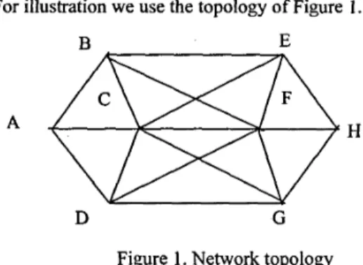
For illustration we use the topology of Figure 1.B E
D G
Figure 1. Network topology
A, B, C,
D,
E, F, G, and H denote the routers. A and H are the two endpoints of a path (A, B, E, H). A computes a threshold value T1= (U/2)(1+
Hurst), where U is the unused, available buffer size in bytes and Hurst is the Hurst parameter of the bursty traffic. The Hurst parameter wassent to A during the connection establishment phase estimated by the originator of the path. The Hurst parameter has been calculated from the application’s profile and previous measurements. Using previous connections, A can also estimate the expected number of packets that could be lost due to the bursty nature of the traffic. When the traffic volume measured in bits/sec exceeds the threshold value
T1, A will disperse the traffic over n new paths leading to
H. A will select the n “best” adjacent routers to split the traffic flow. A sends a request to disperse a portion of the traffic to adjacent routers along with the Hurst parameter and an upper bound on the expected number of dropped
packets. A router is qualified if it has been able to reroute dispersed traffic in previous cases. The routers compute the estimated number of lost packets and calculate the cost of dispersion c>=l. These estimates are sent back to A , which will select n new routes with the smallest estimates as calculated below. For the sake of simplicity we assume n=3, i.e., the connection is dispersed via three routers, e.g., via B, C and D. The cost estimate of a router is based on a performance parameter P, a measure of a router’s inefficiency (as calculated by its predecessor router along the dispersed path) based on its previous traffic dispersions. Small (close to zero) valules of P indicate high quality and efficiency, and high values indicate that the router is unreliable and unstable in rerouting the dispersed circuit. A router’s performance parameter P is recalculated afler each traffic dispersion. The recalculation is based on the statistical evaluation of the router’s estimated and actual number of lost packets [lo]. The motivation for using P is
to enable the selection process to learn from past performances and use this knowledge to select the most efficient routers in traffic dispersion.
The process continues recursively at B, C, and D. At each recursive step all three routers use three arguments: the connection number, the subsequent router, and the upper bound on the number of packets lost. Each step expands the path by those children through which the estimated number of packets does riot exceed the upper bound. Each step returns the estimated number of packets along the path to a child and replaces the parent values with the minimum of the estimated number of packets via the last children expanded. The recursive step goes back along the path, until a better estimate h reached, Then, the procedure continues along that path. After a recursive step these estimates will be equal to the minimum estimated number of dropped packets along the path leading to the last child of the expanded subtree. Once the destination H is reached the selection processes stop. The dispersed paths are along the return paths of the recursive steps. The selection of the dispersed paths is based on estimates and information about the routers’ previous peiformance. Since at each step the path with the estimated least-number of dropped packets is selected, the resulting dispersed paths are expected to be the ones with the least-number of dropped packets. It can be proven that the above algorithm always finds the dispersed paths with the least number of dropped packets if some conditions are met [lo]. (Due to the limited space, this paper does not discus:; the problem of rejoining the
dispersed paths at the destination.) If the traffic’s resource requirement exceeds the router’s total available buffer before the selection for the “best” adjacent routers is completed, then A makes the decision immediately based on data from previous dispersions. The current selection process will refresh A’s records about the “best” neighbors.
2.1
Calculation of the Dispersed Traffic Volumes
Method 1: Let M denote the traffic volume to be dispersed.
Let c l I c2 S
,..,
I ck denote the cost estimates sent by k adjacent routers. Router A will choose the first n 5 k best routers for which M = M/c1+
M/c2+
..+
M/cn, and l/cl+
..
+ l/cn = 1.Method 2: In our simulation we will implement a slightly
modified version of the calculation above. For simplicity, we want to be sure that the traffic is dispersed among the responding k routers proportionally to the available buffer size. A cost estimate ci indicates 1/Ri where
Ri
is the available buffer size of a responding router in bytes, i=l,..,k. Let’s arrange the available buffer sizesR1 1
U?,..
1Rk and compute the s u m R1+
R2+.
..+Rk = R. Disperse the traffic proportionally to the available buffer size:M = M R l R
+
MR2R+
..+
MRn/R, where Rl/R+...
+Rn/R=l.The motivation of A’s decision is that the higher a router’s cost estimate, the lesser amount of traffic will be dispersed via that router.
3.
Simulation Techniques
We assume that the LLbestyy adjacent routers have already been identified by the selection algorithm in [lo]. In order to demonstrate our dispersion algorithm we constructed the following simplified model in COMNET:
/ \
Figure 2. The COMNET model of the network In Figure 2, A, B, C, 0, E, F, G, and H denote the routers of the ATM network connected by OC-3 links: Link AB, Link BE, etc. A is the origin; H is the destination of an ATM
connection. An Application Source called “Bursty Source” attached to router A represents the connection. In COMNET the Application Source contains commands that are executed in sequence when the Application Source is triggered either by time or by received message text. Typically, the command sequence of the Application Source is filled in after the Command Repertoire of the router has been modified to include a desired command. Each router can execute commands and define variables. Commands and variables can be local ones accessed by a router locally or global ones used by any router in the network. A macro is a named collection of commands. The following screen shows the available library commands and the ones defmed for router A:
Figure 3. Library commands and some commands of A The next screen depicts the order of Bursty Source’s commands at router A:
L O W [Tpt) Trampat &e mag to B <-
GLOBAL Ir*tprl t a n p * s R
LOC4L IArgn] Output Paraneter-rnsssue’ IRB/RI LOW [ T p t ] Tr-t d ths m s w a to B 1 x LOCAL IAsgn] Output Paraneter-rqmzeWlRWRI 1 x LOCAL (Tpt)TtmtportRVRdthsmaptustoC 1 x LOCAL egn]Output ParmettcrmJpaze7RDIR) 1 x L O W (Tpt] Trmrpat RD/R d the m t g u n lo D
Figure 4. Command sequence in Phase1 at switch A We give a brief explanation of some commands. For specific details please see [16]. Most of the methods
measuring burstiness are based on the estimate of the Hurst parameter, We implemented the Hurst parameter in COMNET as it is described in [lo]. The first three commands (“Set Pareto Length message,” Set “Output Parameter”, and Transport complete msg to By) generate bursty traffic with Pareto distributed lengths of messages
using the method in [lo]. The following screens show the details of generating Pareto-distributed message lengths with location 8000 and shape 1.1.
Figure 5 . Generating Pareto-distributed lengths of messages These parameters of the Pareto distribution correspond to sending 88000 bytes/sec on the average with Hurst parameter 0.95. (We derived the 8800 byes and the Hurst parameter from real measurements in an ATM network.)
The heavy-tailed Pareto distribution is depicted in the following chart: e , CDF-PDFGraph
la
‘ - .LF.
0 50000 1000001 50000 e I . - PDF-
Par[8000.0,1 .l,O.O) -. CDF-
Par[8000.0.1.1.0.0) I ’ IFigure 6. The heavy-tailed Pareto distribution function In every second the “Bursty Source” application will send a Pareto-distributed length message to the destination. If the message length is less then the threshold T1, A will choose a path via B. Otherwise, it will disperse the traffic among the “best” adjacent routers identified by the selection algorithm illustrated above. For simulation purposes we select T1=10,000 bytes. For simplicity we do not include the selection algorithm in our model, we just assume that these “best”routers are B, C, and
D.
“Bursty Source” will divide the traffic proportionally to the available resources based on the calculation in Method 2 above. The rest of the commands implement the traffic dispersion. Each of the Transport commands will send a portion of the original message to the destination via B, C, and D that isproportional to the buffer size available at these nodes. For instance, the “Transport I W R of the msgsize to B”
command will disperse RB/R portion of the original
message“ to B, where RB -1- RC
+
RD
=R,
and RB, RC, and RD are the available buffer sizes at B, C, and D,respectively. The ‘‘Compute Available Buffer” application executes a command that takes snapshots of the available buffer size of the correspondling router at every second. The next screen shows the application at router B:
Figure 7. The “Compute Available Buffer” application The Compute RB command takes a snapshot of B’s available buffer size. B sends RB to A . Routers C and
D
do the same, sending RC and RD to A , which computes R from the snapshot values. (For reducing the simulation time we limited a router’s maximum. buffer size to 1M bytes only.) The next screen shows the c,alculation:Figure 8. Computing the available buffer size at router B
The “Forward”app1ication forwards the original or dispersed traffic to the destination.
4. Simulation Results
Node
B
C O
D
O
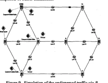
First, we ran the simulation for 1500 seconds without traffic dispersion and measured the buffer utilization and the number of packets dropped at the routers. The following screen shows the animated traffic flow fiom A to H via B and E. The numbers above the routers are the instantaneous snapshots of buffer utilizations.
14
Packets Packets Buffer Buffer Maximum
Accepted Blocked Use Use bytes Avrg. Std
bytes Dev.
1984 189 1536 30683 989274
0 0 0 0
0 0 0 0
Next, we ran the simulation with traffic dispersed via B, C, and D:
/ \
Figure 12. Simulation of dispersed traffic via B, C, and D
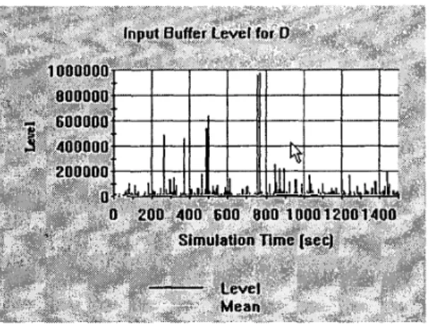
The next screens show the input buffer levels of router B, C, and D:
Figure 9. Simulation of the undispersed traffic via B The next screen shows the input buffer level of router B during simulation:
Figure 13. Input buffer level of router B after traffk dispersion
Figure 10. Input buffer level of router B
Figure 1 1. Number of packets dropped and input buffer
usage
Figure 14. Input buffer level of router C after traffic dispersion
Figure 15. Input buffer level of router D after traffic dispersion
Node Packets Packets Accepted Blocked
B 1623 17 C 1623 17 D 1623 17
Buffer Buffer Maximum Use Use bytes Avrg. Std
bytes Dev.
407 13350 971099 407 13350 971099 407 13350 971099 Figure 16. Number of packets dropped and input buffer
usage after traffic dispersion
In order to eliminate packet drops, A needs to slow down the transmission rate. If we change the 1-second interarrival rate in the “Bursty Source” to 2 seconds the simulation shows that no further packets are dropped.
5.
Conclusion
The paper described an active network algorithm to avoid congestion due to bursty traffic. When the traffic burstiness at a router exceeds a certain threshold calculated as a function of the Hurst parameter and the router’s buffer size, the router will disperse the traffic over n number of new paths leading to the destination of the original traffic. We demonstrated the algorithm’s performance through a discrete event simulation model using Compuware’s COMNET. Our model generates bursty traffic on all time scales based on measurements of a real ATM network. The simulation results show that our algorithm can reduce the number of dropped packets due to the bursty nature of the traffic.
References
[l] Leland, W., Taqqu, M., Willinger, W., and Wilson, D. W., “On the Self-similar Nature of the Ethernet Traffic,” IEEE Transactions on Networking, Vol. 2, no. 1, February 1994, pp.1-15.
[2] R. G. Addie, M. Zukerman, and T. D. Neame, “Broadband Traffic Modeling: Simple Solutions to
Hard Problems,” IEElE Communications Magazine, P. J. Davy, “Self-similar processes with non-negative stationary increments,” submitted to J. of Stat. Planning and Inference.
M. Taqqu, V. Tevlerovsky, and W. Willinger, “Estimators for long-range dependence: an empirical study,” Fractals, Vol. 3, No. 4 1995, pp. 785-788.
S. Molnar, A. Vidacs, and A. Nilsson, “Bottlenecks on the Way towards fractal characterization of Network traffic: Estimation and Interpretation of the Hurst Parameter,” http://hsnlab.ttt.bme.hu/-molnar T. Neame et al., “Investigation of traffic models for high speed data networks,” Proceedings of ATNAC ’95, 1995.
J-C Bolot and A. Shmkar, “Dynamical Behavior of Rate Based Flow Control Systems,” Comp. Commun. Rev., vol. 20, no. 2, ACM SIGCOMM, Apr. 1990. T Faber, “ACC: Using Active Networking to Enhance Feedback Congestion Control Mechanisms,” IEEE Network, May/June 1998, pp.61-65.
E. Gustafsson, “A Literature Survey on Traffic Dispersion,” IEEE Network, March/April 1997, pp. August, 1998, pp.88-95.
28-36.
[lo] Gyires, T., “Smart Permanent Virtual Circuits in Asynchronous Transfer Mode Networks,” invited paper in the Proceedings of the 1997 IEEE International Conference on Systems, Man, and Cybemetics, October 12-1 5, Orlando, Florida, pp. 111 Gyires, T., “Perfo~mance Prediction of Smart Permanent Virtual Circuits in ATM Networks with CACI COMNET,” hi the Proceedings of the 1998 IEEE International Conference on Systems, Man, and Cybemetics, Intelligent Systems For Humans In A Cyberworld, October 11-14, 1998, Hyatt Regency La Jolla, San Diego, California, pp.3993-3998.
121 Gyires, T., “Methodology for Modeling the Impact of Traffic Burstiness on High-speed Networks,” in the Proceedings of the 1999 IEEE Systems, Man, and Cybernetics Conference, October 12-15, 1999, Tokyo, Japan, pp. 980-985.
[13] T. T. Lee and S. C. Liew, “Parallel Communications
for ATM Network Control and Management,” Proceedings of 1EE:E GLOBECOM ‘93, vol. 1, Houston, TX, Dec. 15193, pp. 442-46.
[14] D. Sidhu, S. Abdullah, and R. Nair, “Congestion Control in High Speed Net-works via Alternate Path Routing,” J. High Speed Networks, vol. 1, no. 2, 1992, pp. 129-44.
[15] S. Bahk and M. El Zarki, “A Dynamic Multi-Path Routing Algorithm for ATM Networks,” J. High Speed Networks, vol. 1, no. 3, 1992, pp. 215-36. [16] “COMNET I11 Application Notes: Modeling ATM
Networks with COMNET
III”
CACI Products Company, 3333 North Torrey Pines Ct., La Jolla, California 92037, 19!X[17] V. Paxson, S. Floyd, “Wide Area Traffic: The Failure of Poisson Modeling,’’ IEEE/ACM Transactions on Networking. Vol. 3. NO. 3. June 1995. ~ ~ . 2 2 6 - 2 4 4 .