Contribution to the study of electrostatic properties of proteins from low-resolution electron density distributions and potential functions, Mémoire - Prix de l'Académie Royale de Belgique

RESEARCH OUTPUTS / RÉSULTATS DE RECHERCHE

Author(s) - Auteur(s) :

Publication date - Date de publication :

Permanent link - Permalien :

Rights / License - Licence de droit d’auteur :

Institutional Repository - Research Portal

Dépôt Institutionnel - Portail de la Recherche

researchportal.unamur.be

University of Namur

Contribution to the study of electrostatic properties of proteins from low-resolution electron density distributions and potential functions, Mémoire - Prix de l'Académie Royale de Belgique

Leherte, Laurence

Publication date:

2009

Document Version

Peer reviewed version Link to publication

Citation for pulished version (HARVARD):

Leherte, L 2009, Contribution to the study of electrostatic properties of proteins from low-resolution electron

density distributions and potential functions, Mémoire - Prix de l'Académie Royale de Belgique. Mémoire - Prix

de l'Académie royale de Belgique.

General rights

Copyright and moral rights for the publications made accessible in the public portal are retained by the authors and/or other copyright owners and it is a condition of accessing publications that users recognise and abide by the legal requirements associated with these rights. • Users may download and print one copy of any publication from the public portal for the purpose of private study or research. • You may not further distribute the material or use it for any profit-making activity or commercial gain

• You may freely distribute the URL identifying the publication in the public portal ?

Take down policy

If you believe that this document breaches copyright please contact us providing details, and we will remove access to the work immediately and investigate your claim.

FACULTES UNIVERSITAIRES NOTRE-DAME DE LA PAIX NAMUR

Groupe de Chimie Physique Théorique et Structurale Laboratoire de Physico-Chimie Informatique

Rue de Bruxelles, 61 – 5000 Namur

C

S

E

P

P

L

-R

E

D

D

P

F

Mémoire présenté dans le cadre du Concours Annuel de l’Académie Royale de Belgique Classe des Sciences

Laurence LEHERTE 2009

Préambule

Ce mémoire est introduit auprès de l’Académie Royale de Belgique, Classe des Sciences, en réponse à la question du Groupe III – CHIMIE de l’année 2009 :

« On demande une contribution à l’étude des propriétés électrostatiques dans les molécules, les protéines ou les solides au départ de la fonction de distribution de densité électronique à basse résolution. »

Le sujet qui y est traité concerne l’élaboration de modèles « gros grains » de protéines issus de fonctions de distribution de densité électronique moléculaire lissées et de la fonction dérivée qu’est le potentiel électrostatique moléculaire. Les aspects principaux du travail concernent, d’une part, l’élaboration d’une technique de recherche et d’identification des « gros grains », la détermination de leur charge électrique, et, d’autre part, la validation des modèles au travers d’applications aux systèmes protéiniques.

Foreword

In the present work, we develop protein coarse grain electrostatic models from electron density distribution functions and molecular electrostatic potentials. The main aspects of this work regard, on the one hand, the elaboration of a procedure for the location, the identification, and the charge determination of the coarse grains and, on the other hand, the validation through applications to protein systems.

List of abbreviations

3D Three-dimensional

AA Amino Acid

Amber Assisted Model Building and Energy Refinement

a.u. atomic unit

BAK Backbone

CCDC Crystallographic Data Centre

CG Coarse Grain

c.o.m. Center of mass

CP Critical Point

DNA Desoxyribonucleic Acid ED Electron Density ENM Elastic Network Model

FF Force Field

Gromos GROningen MOlecular Simulation hAr human Aldose reductase

HP7 12-residue β-hairpin peptide KcsA Potassium Ion Channel LJ Lennard-Jones MD Molecular Dynamics

MEP Molecular Electrostatic Potential MOF Minimal Objective Function

NADP Nicotinamide Adenine Dinucleotide Phosphate NMA Normal Mode Analysis

OF Objective Function

PASA Promolecular Atom Shell Approximation PDB Protein Data Base

rmsd Root Mean Square Deviation

rmsdV Root Mean Square Deviation of the electrostatic potential grid values rmsdμ Mean Square Deviation of the molecular dipole moment value

SCH Side Chain

vdW van der Waals

Préambule...1

Foreword ...1

List of abbreviations...2

I. Introduction... 4

II. Topology of Low-Resolution or Smoothed Molecular Electron Density Distributions - Applications ... 9

Electron Density Calculation – Crystallography-Based Approach... 9

Critical Point Analysis ...10

Shape Reconstruction...12

Steric Interaction Energy ...13

Electron Density Calculation – Promolecular Approach... 14

Merging/Clustering Technique ...15

Elastic Network Models...16

Topology of the Molecular Electrostatic Potential... 18

III. Determination of Protein Coarse-Grain Charges from Smoothed Electron Density Distribution Functions and Molecular Electrostatic Potentials... 20

Abstract ... 21

Introduction... 22

Theoretical Background... 24

Smoothing Algorithm ...24

Promolecular Electron Density Distributions ...26

Molecular Electrostatic Potentials ...27

Calculation of Fragment Charges ...27

Results and Discussion ... 29

Protein Backbone Modeling...31

Protein Side Chains Modeling ...38

Application to 12-Residue β-Hairpin HP7...51

Conclusion ... 56

Acknowledgments... 58

References ... 58

IV. Refinement of the Amber-Based CG Model... 61

Selection of the Smoothing Degree ... 61

Application to 12-Residue β-Hairpin HP7... 68

V. Extension to Other Force Fields – Application to the Gromos43A1 Set of Charges ... 73

Selection of the Smoothing Degree ... 73

Application to 12-Residue β-Hairpin HP7... 81

VI. Automation of the CG Generation Procedure – Application to the Potassium Ion Channel KcsA ... 86

VII. Conclusions and Perspectives ... 102

VIII. References ... 105

IX. Appendices... 113

Appendix I. Atom charges as defined in the force field Amber ...113

I. Introduction

Applications of interaction potential functions, parametrized for small or large molecules, require the definition of the electrostatic contributions that commonly involve the determination of atomic point charges. Those contributions are fundamental in that they govern local and global properties, e.g., molecular stability, flexibility, … For macromolecules, the sampling of conformational space is however a complex and highly time-consuming task due to the large number of degrees of freedom of the systems and the complexity of the interaction potential functions. It is nevertheless a major interest to relate a protein function to its microscopic description, notably for the study of protein-protein and protein-ligand interactions. For recent years, much effort has been put into accelerating computational techniques such as Molecular Dynamics (MD) and Normal Mode Analysis (NMA) for simulating large biological systems [emp08, hin08, mor08]. Enhancements to these well-known algorithmic procedures are based, notably, on a spatial coarse graining of the molecular structures [vot09]. Rather than simulating the molecules at their atomic level, one reduces their description to a limited set of points, either centered on selected sites/atoms such the Cα atoms of a protein backbone [dor02, emp08], the center of mass (c.o.m.) of specific groups of atoms like amino acid (AA) residues [bas07], the heavy atoms (united atom description) [fuk01, yan06], or a set of merged atoms [goh06]. Elastic Network Models (ENMs) are among those NMA methods wherein coarse grains (CGs) are interacting through harmonic potential functions. Despite their simplicity, sometimes based on the topology of the protein structure only (excluding inter-CG distance information), they have shown to be extremely useful for the modeling of slow large amplitude motions of proteins [kon06, cle08]. It has even been demonstrated that grouping up to 40 residues into a single node essentially produced the same low-frequency modes as the original single Cα node per residue [dor02]. In a very recent work, Zhang et al. [zha08] proposed a method to define CGs that reflect the collective motions computed by a Principal Component Analysis of an atomistic MD trajectory. Each CG site is the c.o.m. of a domain, i.e., a group of contiguous Cα atoms that move in a highly correlated fashion. Reviews of the progresses on CG-ENM and -MD models can be found in references [chn08, yan08] and in the Introduction of Section III.

Besides the use of simple harmonic functions, the development of CG interaction potential functions is generally made either from atomistic interaction potential [par05] or MD results [izv05,

liu07, car08], via experimental data such as B-factors [kon06], or through the fitting of a potential function achieved by matching CG and atomistic distributions [fuk01, car08]. For example, Lyman et al. [lym08] presented a new method for fitting spring constants to mean square CG-CG distance fluctuations computed from atomistic MD. One can also cite the Inverse Monte Carlo approach [lyu95], used for iteratively adjusting an effective CG potential function until it matches a target radial distribution function. Consistency between CG and all-atom models can be checked through a statistical mechanics theory as proposed by Noid et al. [noi08a, noi08b]. Another example is the parametrization of the MARTINI force field (FF), dedicated to MD simulations of biomolecular systems, and based on the reproduction of partitioning free energies between polar and apolar phases of a large number of chemical systems [mar07, mon08]. The model is based on a four-to-one mapping, i.e., four heavy atoms are represented by a single interaction center, except for small ring-like fragments (Figure I.1). Specifically, AAs consist of one to four side chain beads and one backbone bead [mon08]. Only four main types of interaction sites are defined: polar (P), non-polar (N), apolar (C), and charged (Q). Each particle type has a number of subtypes, which allow for an accurate representation of the chemical nature of the underlying atomistic structure. In the MARTINI FF, only AA residues Arg, Asp, Glu, and Lys, are charged. Such a description was for example applied to protein channels embedded in a lipid membrane environment [tre08].

Figure I.1. Illustration depicting MARTINI CG models for molecular structures of various sizes. The illustration is taken from [http://md.chem.rug.nl/~marrink/coarsegrain.html].

In the UNRES model [liw09], a peptidic chain is represented by a sequence of backbone beads located at peptide bonds, while side chains are modelled as single beads attached to the Cα atoms, which are considered only to define the molecular geometry. In the so-called SimFold CG description and energy function, a mixed representation is used. Residues of aqueous proteins are represented by backbone atoms N, Cα, C, O, and H, and one side chain centroid [fuj04, hor09]. In UNRES and SimFold, electrostatic interactions are not explicitely calculated using the Coulomb term like they are in the MARTINI FF.

Multiscale methods, that combine several levels of description, are also appealing since they allow to model limited regions of space with details while limiting the outer regions to coarser models [cle08, she08]. Besides their limitations, i.e., simplified interaction potential functions, neglect of fast motions, faster dynamics than all-atom systems, or partial rigidity of the structure, many studies have found good conformational sampling agreement between features predicted by NMA, for instance, and the observed or simulated conformational change of protein structures, as reported in [dob08]. The consideration of external influences, such as external stresses [eya08] or solvent effects [zho08] can also be treated with CG approaches.

Our first studies on the interaction potential of CG molecular representations, achieved in the frame of a post-doctoral stay at the Cambridge Crystallographic Data Centre (CCDC), were dedicated to a DNA-drug system [leh94]. In that work, a computational method was described for mapping the volume within the DNA double helix structure that is accessible to netropsin, an antitumor antibiotic drug molecule that binds in the minor groove of DNA. Based on a topological analysis of the electron density (ED) of both the DNA and the drug molecule, calculated at a crystallographic resolution of 3 Å, a Lennard-Jones (LJ) type interaction potential was implemented to evaluate the interaction energy of a spherical probe and a DNA structure represented by a limited number of ellipsoids. It was concluded that the global shape of a molecule could be described using local information associated with its centers of high ED, i.e., peaks expanded in terms of ellipsoids. The idea was later extended to the study of supramolecular cyclodextrin-based systems [leh95], zeolitic frameworks [leh97], and protein and DNA complexes [bec03].

In a further comprehensive work, this theory was expanded to model protein-protein and protein-DNA complementarity [bec04b]. The strategy implemented to dock the partners was based on the use of the hereabove mentioned reduced dimensionality representations of biological macromolecules combined with a genetic algorithm. One of the main objectives consisted in the development of an intermolecular interaction function specifically adapted to reduced molecular

studies of protein-protein and protein-DNA complexes of known structures. The interaction function was a combination of the contact interface area, an electrostatic interaction potential, a steric clash detection procedure, and a contribution related to the macromolecular recognition. This last term was based on a set of distribution tables of preferential distances constructed from statistical analyses of 475 protein-protein complexes and 165 protein-DNA complexes [bec04a, bec07]. The electrostatic potential consisted in a summation over unit charges assigned to the charged residues such as Arg, Lys, Asp, and Glu.

Our first attempt to assign non unitary electric charges to ED peaks was achieved through a collaborative work with the members of the Laboratoire de Cristallographie of the Université de Nancy, directed by Prof. Cl. Lecomte [leh07]. ED distribution of the adenine binding site of the human Aldose reductase (hAr) protein structure and its cofactor NADP+ were calculated using a promolecular analytical approach. ED peaks were located by following the atom trajectories in progressively smoothed ED distributions using a merging/clustering algorithm. To each maxima, it was possible to define their corresponding molecular fragment through a clustering procedure. Molecular electrostatic potentials (MEPs) generated by the adenine binding site in the hAr structure and the electrostatic interaction energies of the adenine moiety with the protein binding site were calculated using several charge models. Two models were built from two sets of atomic charges derived from subatomic resolution XRD data. Each of these two sets was used to calculate the electric charge of ED-based protein fragments centered at ED maxima. An additional charge model was built by assigning formal unit charges to the Arg(+1), Lys(+1), Glu(-1), and Asp(-1) side chains.

Later, the modelling of flexible protein structure was achieved using NMA-based approaches, more specifically ENMs with force constants weighted by the overlap integral value of the fragment ED distribution functions [leh08a, leh08b].

Following our development of an original approach to hierarchically decompose a protein structure into fragments from its ED distribution [leh04, leh07], the method is here applied to MEPs, calculated from point charges as implemented in well-known force fields. To follow the pattern of local maxima and minima in a MEP, as a function of its resolution/degree of smoothing t, the following strategy was adopted. First, each atom of a molecule is considered as a starting point. As the smoothing degree increases, each point moves along a path to reach a location where the MEP gradient value vanishes. Convergence of trajectories leads to a reduction of the number of points. Practically, to determine the protein backbone representations, we analyzed CG models obtained for a β-strand of 15 glycine residues. A fitting algorithm was used to assign charges to the obtained

local maxima and minima vs. the unsmoothed MEP, as a function of t. The best fit obtained allowed to determine the degree of smoothing to be considered. Then, the influence of the different AA side chains was studied at the selected value of t for different rotamers by substituting the central glycine residue.

A description of the basic theory is reported in Section II of the present document. Section III consists in the reproduction of our first comprehensive research work about the analysis of smoothed Amber-based MEP and the determination of CG point charge models applicable to protein structures. In Sections IV and V, we report how to improve CG models built from smoothed MEP, and we extend that approach to the set of charges used in the FF Gromos43A1. An automated procedure to generate electrostatic CG representations of proteins is then described in Section VI and applied to a large ion channel protein system. Finally, general conclusions and perspectives, that include a discussion about transferability, are presented in Section VII.

II. Topology of Low-Resolution or

Smoothed Molecular Electron Density

Distributions - Applications

In this Section, we present the fundamental concepts and procedures that are useful for the understanding of our approach. They complete the Theoretical Background part that appear in Section III; some redundancies may thus occur.

Electron Density Calculation – Crystallography-Based Approach

The intensity of X-rays diffracted by a crystalline structure is proportional to the modulus of their corresponding structure factor F(h):

) ( ) ( ) ( h h h F e iϕ F = − (1)

where h is a reciprocal space vector with indices h, k, and l, an φ(h) is the phase of the diffracted wave. Within the crystallographic approach, the electron density (ED) distribution function ρ(r) is calculated as the Fourier Transform of F(h):

{ }

∑

V being the volume of the unit cell. Such ED maps can be calculated at various resolution levels through the simulation of X-ray diffraction experiments using programs such as XTAL [hal90].

In practice, the number of known structure factors occurring in equation (2) is not infinite and varies with the resolution. In crystallography, the resolution factor dmin is a well-known

min max 2 1 ) sin ( d = λ θ (3) where 2θ is the angle between the diffracted and the primary beams of wavelength λ, and dmin

depends on different parameters including the quality of the crystal, the chemical composition, the radiation used, and the temperature of the experiment. For example, Figure II.1 depicts the ED distributions of the Diazepam molecule calculated using XTAL at various resolution levels.

Figure II.1. Iso-contours of the ED distributions calculated for Diazepam using XTAL at a resolution of (left) 2.5 Å (iso = 1.5, 2, 3 e-_/Å3_{) and (right) 3.0 Å (iso = 1.2, 1.5, 1.9 e}-_/Å3_{), with superimposition on the local maxima (black spheres)}

and saddle points (white spheres).

Critical Point Analysis

An ED distribution ρ(r) can be described in terms of the location and identification of its critical points (CPs), i.e., points where the gradient of the density is equal to zero. They are thus characterized as maxima, minima, or saddle points depending upon the sign of the second derivatives of ρ(r). The Hessian matrix H of a continuous 3D function such as the ED is built from its second derivatives:

⎟⎟ ⎟ ⎟ ⎟ ⎟ ⎟ ⎟ ⎠ ⎞ ⎜⎜ ⎜ ⎜ ⎜ ⎜ ⎜ ⎜ ⎝ ⎛ ∂ ∂ ∂ ∂ ∂ ∂ ∂ ∂ ∂ ∂ ∂ ∂ ∂ ∂ ∂ ∂ ∂ ∂ ∂ ∂ ∂ ∂ ∂ ∂ = 2 2 2 2 2 2 2 2 2 2 2 2 z y z x z z y y x y z x y x x ρ ρ ρ ρ ρ ρ ρ ρ ρ H (4)

This real and symmetric matrix can be diagonalized. The three resulting eigenvalues provide informations relative to the local curvature; the Laplacian ∇2ρ(r), which is the summation over the

three eigenvalues, gives details about the local concentration (sign < 0) or depletion (sign > 0) of the ED. If the rank (number of non zero eigenvalues) of the diagonalized matrix is 3, then four cases are met. The signature (sum of the sign of the eigenvalues) s = -3 corresponds to a local maximum or peak, i.e., the ED function adopts maximum values along each of the three principal directions x', y', and z'. s = -1 corresponds to a saddle point or pass where two of the eigenvalues are negative; these are also called Bond Critical Points. s = +1 corresponds to a saddle point or pale characterized by only one negative eigenvalue. s = +3 corresponds to a local minimum or pit, i.e., the ED function adopts minimum values along each of the three principal directions.

Morse theory allows to determine whether the set of critical points is topologically consistent. It is applicable to functions which are everywhere twice differentiable, and wherein there is no degenerate critical points, i.e., no zero eigenvalues of the Hessian matrix at the critical point locations. Considering Mk as the number of CPs with index k of the function ρ(r), then:

1 0 1 2 3−M +M −M = M (5)

where M3, M2, M1, and M0 stand for the number of peaks, passes, pales, and pits, respectively

[lio93]. In the case of crystals, the CP network is defined not only by the molecular structure but also by the lattice periodicity and the space group symmetry. Due to periodic boundary conditions, a unit cell can be considered as a 3D torus, each pair of opposite faces being connected. This means that the motif of CPs is not isolated but interacts with its periodic images and, therefore, the number of CPs is constrained by the relationship:

0 0 1 2 3−M +M −M = M (6)

At atomic resolution, peaks and passes are normally associated with the presence of atoms and chemical bonds, respectively, while pales and pits occur as a result of the geometrical arrangement of the atoms and the corresponding networks of bonds. Pales and pits are found in the interior of rings and cages, respectively [bad95]. Figure II.2 represents a cubic network of CPs, with one peak located at each of the 8 corners. The 8 Gaussian functions built on these peaks generate a pass on each of the edges, pales centered on the 6 faces, and one pit located in the center of the cube.

Figure II.2. Critical point network ‘peak (red) – pass (yellow)’ and ‘pit (dark blue) – pale (light blue)’ of a cubic arrangement of three-dimensional Gaussian functions.

Shape Reconstruction

At the CP locations, the three main curvatures of the ED function are the eigenvalues of the Hessian matrix constructed from the second derivatives. It is assumed that this local information can be transferred to the space surrounding the CP concerned; hence it is possible to evaluate (or reconstruct) the 3D function in the close neighbourhood of each point. Each maximum of the ED function, i.e., each peak, is considered as the center of expansion of a Gaussian function and such a mathematical expression is fitted in order to define a volume around each peak taking into account its three characteristic eigenvalues:

0 ' 0 ) ( ρ α ρ ρ r H r r T e = (7)

where H’ is the diagonalized form of H, and r is defined in a reference frame built on the three corresponding eigenvectors. In order to evaluate the volume associated with a particular peak, the exponential term of the Gaussian function can be integrated over the space within the frame of an ellipsoid:

∫

characterized by three main axes rX, rY, and rZ:

Z Y X Z Y X r r r h h h V 4₃ 2 / 3 2 / 3 0 2 / 3 2 π ρ π = = (9)

and hence provides a method of representing shape anisotropy of the CPs. This shape description is extended to a whole molecule by considering a set of ellipsoids, and a descriptor for the resulting structure can be defined in terms of interaction energy values, as described below.

Steric Interaction Energy

In a study on the DNA-netropsin system [leh94], the total interaction energy E between the host ellipsoids and a guest probe was expressed within a pseudo-pair potential approximation, wherein the dispersive interaction between an ellipsoid i and a sphere j is proportional to their volume product: 12 6 ij ij ij ij ij r B r A E =− + where Aij > 0 and Bij > 0 (10) j i ij VV A = (11) 6 ) ( _{i j} ij ij A r r B = + (12)

rij being the separation distance between particles i and j, and ri and rj, their radius calculated along

the interdistance vector i-j. In such a formula, it is considered that the equilibrium distance between i and j is given by 21/6(r_i +r_j)and Eij = 0 when r_ij =

(

)

pseudo-potential energy function to determine the optimal steric location of a guest molecule was also developed by Kuntz and coworkers [sho93, gro94, goo95] in the program DOCK. These authors simplified the overlap energy between two molecules to a contribution depending upon the van der Waals (vdW) radii of the interacting atoms and their separation distance. Considering a LJ type potential allowed us to emphasize the effect of global curvature of the neighbourhood, e.g., a cavity leading to more attractive energies. Fitting Gaussian functions to a higher resolution representation, i.e., to atoms, has been done latter by Grant and Pickup [gra95] to overcome the limitations of hard sphere representations of molecular shapes. From such functions, these authors were able to derive gradients and Hessian of the nuclear coordinate derivatives, i.e., properties similar to CP characteristics.

Electron Density Calculation – Promolecular Approach

Promolecular models have often turned out to lead to very good approximated representations of ED distributions for the purpose of a number of applications as varied as chemical bond analysis or molecular similarity applications for example [tsi98a, tsi98b, gir98, mit00, gir01, dow02, bul03]. In the Promolecular Atomic Shell Approximation (PASA) approach, a promolecular ED distribution

ρM is calculated as a weighted summation over atomic ED distributions ρa, which are described in

terms of series of squared 1s Gaussian functions fitted from atomic basis set representations [ama97]:

(

)

where Ra is the position vector of atom a, and wa,i and ζa,i are the fitted parameters, respectively, as

reported in the Web site at [http://iqc.udg.es/cat/similarity/ASA/funcset.html]. ρM is then calculated

as: ∑ = a a a M Z ρ ρ (14)

where Za is the atomic number of atom a.

In one of our approaches to generate low resolution 3D functions [leh01], an ED map is a deformed version of ρM that is directly expressed as the solution of the diffusion equation according

to the formalism presented by Kostrowicki et al. [kos91]:

(

)

b_{ai ai a,i a,i} a,i _⎟⎟

⎠ ⎞ ⎜⎜ ⎝ ⎛ = = ς (16)

In this context, t is seen as the product of a diffusion coefficient with time. It has also been shown that t is equivalent to the well-known crystallographic anisotropic displacement parameter u2

[leh04]. Figure II.3 shows the evolution of the ED distribution of Diazepam calculated at the RHF-MO-LCAO 6-31G* level as t increases from 0.0 bohr2 (original PASA distribution) to 2.5 bohr2.

Figure II.3. Iso-contours of the ED distributions calculated for Diazepam at the PASA level with (top left) t = 0.0 bohr2 _{(iso =}

0.1, 0.2, 0.3 e-_/bohr3_{), (top right) t = 1.1}

bohr2 _{(iso = 0.1, 0.15, 0.2 e}-_/bohr3_{), (bottom}

left) t = 1.6 bohr2 _{(iso = 0.10, 0.125, 0.15 e}

-/bohr3_{), and (bottom right) t = 2.5 bohr}2 _(iso

= 0.05, 0.075, 0.10 e-_/bohr3_{), with}

superimposition on the local maxima (black spheres) and saddle points (white spheres).

Merging/Clustering Technique

One way to follow patterns of CPs, and more particularly of the peaks, as a function of the degree of smoothing is to implement the algorithm proposed by Leung et al. [leu00]. These authors proposed a method to model the blurring effect in human vision. This was achieved (i) by filtering a digital image p(x) through a convolution product with a Gaussian function g(x,t):

2 2 ₂ 2 1 ) , ( e x t t t x g = − π (17)

where t is the scale parameter, and (ii) by assigning each data point of the resulting p(x,t) image to a cluster via a dynamical equation built on the gradient of the convoluted image:

) , ( ) ( ) 1 (n x n h p x t x + = + ∇_x (18)

where h is defined by the authors as the step length. We have adapted this idea to 3D images such as PASA ED distribution functions. In this framework, the original ED corresponds to the PASA ED approximation at scale t = 0 where each atom of a molecular structure is considered as the

starting points of a merging procedure. As t increases continuously from 0.0 to a given maximal value, each peak moves continuously along the gradient path to reach a location in the 3D space where ∇ρ = 0.

On a practical point of view, this consists in following the trajectory of the peaks obtained at a resolution (t - Δt) on the ED distribution surface calculated at resolution level t. Once all peak locations are found, close peaks are merged and the procedure is repeated for each selected value of t until the whole set of maxima becomes one single point.

The results obtained using this algorithm can be visualized in terms of dendrograms via the program Phylodendron [gil96]. The dendrogram obtained for the Diazepam molecule and the corresponding significant substructures, i.e., the chlorine atom (I), the carbonyl function (II), the imine group (III), and the phenyl moiety (IV), are shown in Figure II.4.

Figure II.4. (left) Dendrogram obtained from the hierarchical merging/clustering procedure applied to PASA ED maps of Diazepam; results at t = 1.1, 1.6, 1.9, and 2.5 bohr2 _{are emphasized using vertical lines. (right) Contours of the}

molecular fragments shown at resolution values t = 1.1 (plain line), 1.6 (long dashed line), 1.9 (dash-dot line), and 2.5 bohr2 _{(dotted line).}

Elastic Network Models

Normal Mode Analysis (NMA) is a classical technique for studying the vibrational (and thermal) properties of molecular structures. Although this technique is widely used for molecular systems consisting of a small number of atoms, performing NMA on large-scale systems, as proteins, is computational challenging, and reduced representations, often based on Cα atoms only, are used

(Figure II.5). So-called Elastic Network Models (ENM) are, for example, built by connecting the neighboring residues of a protein by springs with a harmonic and uniform force constant.

Figure II.5. Illustration of an ENM for lysozyme using a Cα representation (green spheres). The interactions are represented by springs (in red) between pairs of atoms. Figure is taken from [Hinsen, K., Elastic Network Models for Proteins, Theoretical Biophysics, Molecular Simulation, and Numerically Intensive Computation,

http://dirac.cnrs-orleans.fr/plone/Members/hinsen/elastic-network-models-for-proteins, 2007].

Mathematically, the motion of the molecule can be described by a second order ordinary differential equation:

0 = + rF

r&& (19)

where the matrix F is a force constant matrix built from the second derivative of the potential with respect to the Cartesian coordinates. The standard procedure for solving this equation is to diagonalize the matrix F by computing its eigenvalues and eigenvectors. Each eigenvector is often referred to as a normal mode with a vibrational frequency ω, determined by the eigenvalue. The overall dynamics of the molecular system can be described by a superposition of a number of linearly independent normal modes. When working with CG representations, the low-frequency region of the spectrum is particularly interesting because it has been shown that the lowest modes are able to capture collective conformational changes that are hard to access by all-atom MD simulations. In NMA, once the normal mode vectors, their frequencies, and their amplitudes are obtained, various properties can be calculated easily, such as the mean fluctuations of atom positions and their mutual correlations.

In recent studies [leh08a, leh08b], we have evaluated the suitability of smoothed PASA ED overlap integrals:

∫

to model force constants associated with springs between ED fragments centered on ED maxima (peaks). It was verified that the decomposition of a 3D protein structure based on its ED smoothed at t = 1.4 bohr2 allowed to describe its structure in terms of backbone and side chain fragments, each associated with an ED peak. This description is comparable to a representation obtained at a crystallographic resolution value of about 3 Å. ENM built from the backbone ED maxima are thus similar to models built from Cα coordinates.

Topology of the Molecular Electrostatic Potential

Topological analysis of scalar fields other than ED distributions is not very common. Calculations applied to 3D properties, such as molecular electrostatic potentials (MEPs), have nevertheless been proposed by Gadre et al. [gad96] and Leboeuf et al. [leb99].

MEP, a well-known property of a free molecule for examining its reactivity towards nucleophiles, is derived from its molecular ED ρA(r)as:

' ) ' ( ' ) ( r r r r R r r − − − =

∑

∫

where a, Za, and Ra stand for the atoms that constitute the molecular structure A, their atomic

numbers, and their vector positions, respectively. Gadre et al. [gad96] used MEP topology as a predictive tool for obtaining intermolecular interaction parameters. Leboeuf et al. [leb99] showed how MEP CPs are related to the electronic structure (π bonds, lone pairs, …) of the investigated molecules. Pathak and Gadre [pat90] particularly showed that MEP distributions generally lack non nuclear maxima. Politzer et al. proposed procedures for predicting sites of nucleophilic attack, such as the use of a MEP of a molecule in a distorded geometry [pol82], or the mapping of MEP values onto a 0.002 a.u. ED isosurface [sjo90]. If promolecular representations, based on non interacting spherical atoms, are not adapted for predicting interactions sites of molecules, they however provide acceptable results for the analysis of MEP minima along the internuclear axes in a molecule [pac92, bot98]. More recently, but in a less direct work on the topology of MEPs, Popelier et al. [pop04] studied the electrostatic potential generated by the ED of molecular fragments of retinal and lysine

Mata et al. [mat07] reported that zero-flux surfaces occurring in a MEP, as for ρ(r), are also observed between atoms, but the actual partition of the space in volumes is different from that of the ED. They reported a topological analysis procedure for the EP. In the case of MEP, the gradient and Laplacian operators have a particular physical significance. The gradient of V(r) is the negative of the electrostatic field while the Laplacian is related to the density distribution ρ(r) by the Poisson equation: ) ( 4 ) ( 2 r r =− πρ ∇ V ₍₂₂₎

According to Leboeuf et al. [leb99], the Poincaré-Hopf relationship that is valid for MEPs is:

− + + = − + −M M M M M M_{3 2 1 0 (23)}

where M+ and M- stand for the number of asymptotic maxima and minima, respectively. They

correspond to regions of solid angle where V(r) is going asymptotically to zero from positive and negative values, respectively. In the case of the ED, M+ = 1 and M- = 0. In their work, Mata et al.

[mat07] associated each local maxima (nuclei) and minima to electrophilic and nucleophilic sites, respectively, with the corresponding basins indicating their influence zones.

Equation (23) has recently been revisited and generalized by Roy et al. [roy08]. By iteratively visualizing the direction of the MEP gradient calculated on spherical surfaces centered at various molecular points, the authors determine the critical points of the MEP function. The resulting Euler characteristic EC is defined as:

i

n n

EC= ₀ − (24)

where n0 and ni stand for the number of regions on a spherical surface where the MEP increases (the

III. Determination of Protein Coarse-Grain

Charges from Smoothed Electron

Density Distribution Functions and

Molecular Electrostatic Potentials

Original paper accepted in “Computational Chemistry: New Research”, Ed. F. Columbus, Nova Publishers, Aug. 26th 2008.

Determination of protein coarse-grain charges from smoothed electron density

distribution functions and molecular electrostatic potentials

Laurence Leherte, Daniel P. Vercauteren Laboratoire de Physico-Chimie Informatique Groupe de Chimie Physique Théorique et Structurale

University of Namur (FUNDP) Rue de Bruxelles, 61 B-5000 Namur (Belgium)

Abstract

The design of protein coarse-grain (CG) models and their corresponding interaction potentials is an active field of research, especially for solving problems such as protein folding, docking, … Among the essential parameters involved in CG potentials, electrostatic interactions are of crucial importance since they govern local and global properties, e.g., their stability, their flexibility, …

Following our development of an original approach to hierarchically decompose a protein structure into fragments from its electron density (ED) distribution, the method is here applied to molecular electrostatic potential (MEP) functions, calculated from point charges as implemented in well-known force fields (FF). To follow the pattern of local maxima (and minima) in an ED or a MEP distribution, as a function of the degree of smoothing, we adopted the following strategy. First, each atom of a molecule is considered as a starting point (a peak, or a pit for negative potentials in a MEP analysis). As the smoothing degree increases, each point moves along a path to reach a location where the ED or MEP gradient value vanishes. Convergences of trajectories lead to a reduction of the number of points, which can be associated with molecular fragments.

Practically, to determine the protein backbone representations, we analyzed CG models obtained for an extended strand of polyglycine. The influence of the different amino acid side chains was then studied for different rotamers by substituting the central glycine residue. Regarding

the determination of charges, we adopted two procedures. First, the net charge of a fragment was calculated as the summation over the charges of its constituting atoms. Second, a fitting algorithm was used to assign charges to the obtained local maxima/minima.

Applications to a literature case, a 12-residue β-hairpin peptide, are also presented. It is observed that classical CG models are more similar to ED-based models, while MEP-based descriptions lead to different CG motifs that better fit the MEP distributions.

Introduction

The design of coarse-grain (CG) models [1] and their corresponding potential functions [2] for protein computational studies is currently an active field of research, especially in solving long-scale dynamics problems such as protein folding, protein-protein docking, … For example, to eliminate fast degrees of freedom, it has been shown that one can rely on CG representations only, or on mixtures of CG and more detailed descriptions [3,4] in order to significantly increase the time step in molecular dynamics (MD) simulations. Among the parameters involved in CG potentials, the electrostatic interactions are of major importance [5] since they govern local and global properties such as their stability [6], their flexibility [7], …

Common approaches used to design a CG description of a protein consist in reducing groups of atoms into single interaction sites. For example, in reference [8], each amino acid (AA) is represented by a single spherical site, with unit or nul electric charge. The authors studied a proline-rich protein PRP-1 interacting with a mica surface using Monte-Carlo simulations. Curcó et al. [9] developed a CG model of β-helical protein fragments where the AAs are represented by two, three, or four blobs depending upon the AA type, in accordance with a best fitting between Monte-Carlo based all-atom and CG energies. In their work, the AAs are depicted by the amide hydrogen atom HN, the oxygen atom, the geometric center of the side chain (except for Gly), and a fourth blob whose position depends on the AA type (except for Gly, Ala, and Val). In reference [10], each AA residue is modeled using one sphere located on the geometric center of the backbone and one or two spheres located on the geometric centers of the side chain fragments (except for Gly). Differently, Pizzitutti et al. [11] represented each AA of a protein sequence by a charged dipolar sphere. For each AA, one CG sphere is located on the center-of-mass (c.o.m.) of the uncharged residues, while two CG spheres are assigned to the c.o.m. of the neutral part of the AA residue and to the c.o.m. of the charged part, respectively. Charged residues are Lys, Arg, Glu, Asp, and terminal AAs. The

authors show that, in protein association, their model provides a good approximation of the all-atom potential if the distance between the protein surfaces is larger than the diameter of a solvent molecule.

As mentioned earlier, a CG potential can be combined with an all-atom potential. For example, Neri et al. [3] included a CG description, in which the potential energy is expressed as harmonic terms between close Cα and/or Cβ atoms. Such elastic network representations are well-known to study the slow large amplitude dynamics of protein structures [12-15]. The small biologically relevant region of the protein is modeled using an atom-based potential while the remaining part of the protein is treated using a CG model. In this context, Heyden and Thruhlar [16] proposed an algorithm allowing a change in resolution of selected molecular fragments during a MD simulation, with conservation of energy and angular momentum. A different and relatively logic way of considering the combination between all-atom and CG potentials is to use CG as a pre-processing stage carried out to establish starting conformations for all-atom MD simulations [4].

Even when one uses an all-atom representation to model a protein structure, a reduced set of Coulomb charges can still be used. For example, Gabb et al. [17] reported protein docking studies where electrostatic complementarity is evaluated by Fourier correlation. Charges used in Coulomb electrostatic fields were close to unit charges and placed on a limited set of atoms. Besides the use of unit charges as in [8,11,18], an approach to assign an electrostatic charge to a fragment or pseudo-atom is to sum over the corresponding atomic charges. Extended approaches involve the assignment of dipolar and quadrupolar contributions to the CGs [19]. In this last work [19], dedicated to small molecules such as benzene, methanol, or water, the charge distribution is represented by point multipolar expansions fitted to reproduce MD simulation data. Without being exhaustive, other assignment methods consist in fitting the CG potential parameters so as to reproduce at best the all-atom potential values [9,19].

In this chapter, we present two approaches to design and evaluate CG electrostatic point charges. The first one has already been described in a previous work regarding the evaluation of the electrostatic interactions between Aldose Reductase and its ligand [20]. In that first approach, the fragment content is determined through a merging/clustering procedure of atom trajectories generated in progressively smoothed electron density (ED) distribution functions. The specific use of a Gaussian promolecular representation of an ED, i.e., a model where a molecule is the superposition of independent and spherical atoms, allows a fast evaluation of the ED distribution as well as their derived properties such as derivatives and integrals. In the second approach, atoms are clustered according to their trajectories defined in a smoothed molecular electrostatic potential

(MEP) function. As the charge calculation approach useful in ED cases revealed to be inefficient in MEP cases, a fitting algorithm is applied to evaluate CG charges. Results are presented for the 20 AAs, first as derived from a promolecular ED representation, and second from the all-atom Amber charges reported in Duan et al. [21]. In this last work, the authors developed a third-generation point charge all-atom force field for proteins. Charges were obtained by a fitting to the MEP of dipeptides calculated using B3LYP/cc-pVTZ//HF/6-31G** quantum mechanical approaches in the PCM continuum solvent in a low dielectric to mimic an organic environment similar to that of the protein interior.

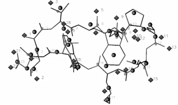
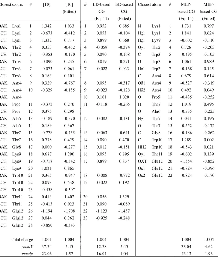
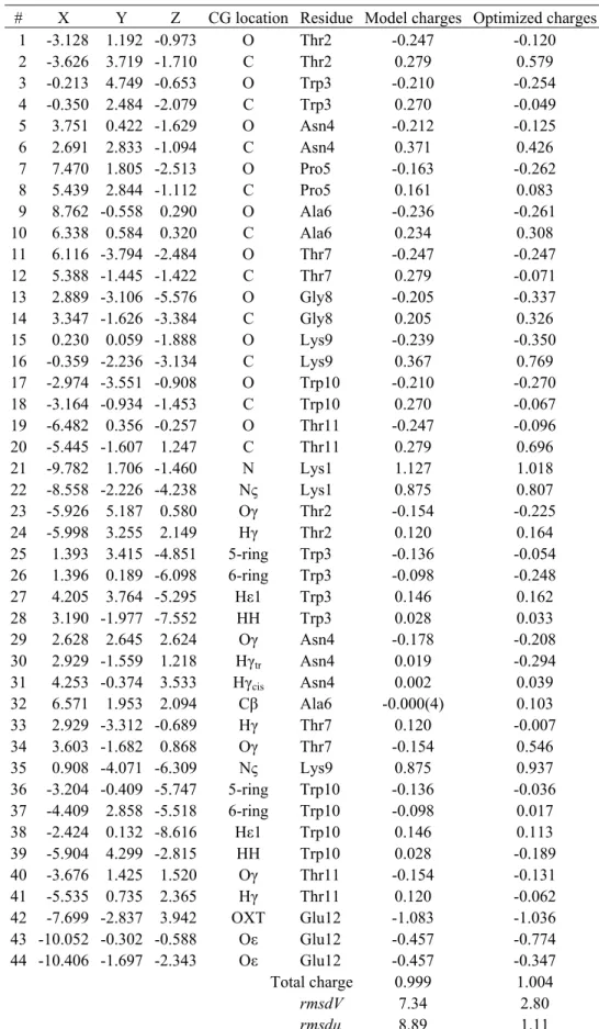
Finally, we will show that the CG charges obtained for each AA residue can be used to determine a CG model representation for any protein. A particular application to a literature case, a 12-residue β-hairpin HP7 [10], is described and MEP results are compared with published models.

Theoretical Background

In this section, we present the mathematical formalisms that were needed to design a protein CG representation and its point charges. First, the smoothing algorithm that is applicable to both ED and MEP functions is described. This description is followed by the mathematical expressions needed to smooth either a Gaussian-based ED distribution function, or the Coulomb electrostatic interaction function. Finally, the two approaches used to calculate CG point charges, from ED- and MEP-based CG, respectively, are detailed.

Smoothing Algorithm

An algorithm initially described by Leung et al. [22] was implemented to follow the pattern of local maxima in a Gaussian promolecular ED or a MEP function, as a function of the degree of smoothing. More particularly, the authors proposed a method to model the blurring effect in human vision, which is achieved (i) by filtering a digital image p(x) through a convolution product with a Gaussian function g(x,t): 2 2 ₂ 2 1 ) , ( e x t t t x g = − π ₍₁₎

) , ( ) ( ) 1 (n x n h p x t x + = + ∇_{x (2)}

where h is defined as the step length. We adapted this idea to three-dimensional (3D) images such as ED and MEP functions, f, such as:

) ( ) ( ) ( ) ( r _{f t} f t rr_{f t} =r_{f t−Δt} + Δ ∇r (3)

where rr stands for the location vector of a point in a 3D function. The various steps of the resulting merging/clustering algorithm are:

1. At scale t = 0, each atom of a molecular structure is considered as a local maximum (peak) of the ED and/or a local minimum (pit) of the MEP function. All atoms are consequently considered as the starting points of the merging procedure described below.

2. As t increases from 0.0 to a given maximal value tmax, each point moves continuously along

a gradient path to reach a location in the 3D space where∇ trf( )=0. On a practical point of view, this consists in following the trajectory of the peaks and/or pits on the ED or MEP distribution surface calculated at t according to Equation (3). The trajectory search is stopped when ∇rf(t) is lower or equal to a limit value, gradlim. Once all peak and/or pit locations are found, close points are

merged if their interdistance is lower than the initial value of Δ1/2. The procedure is repeated for each selected value of t.

If the initial Δ value is too small to allow convergence towards a local maximum or minimum within the given number of iterations, its value is doubled (a scaling factor that is arbitrarily selected) and the procedure is repeated until final convergence.

The results obtained using that algorithm are the location of the local maxima and/or minima, i.e., peaks and pits, and the atomic content of all fragments, at each value of t between 0 and tmax

[23], that can be further interpreted in terms of dendrograms as, for example, using the Web version of the program Phylodendron [24]. For information, input data were written in the adequate format using DENDRO [25], a home-made program implemented using Delphi, an object-oriented programming language that allows the representation and processing of data in terms of classes of objects.

Promolecular Electron Density Distributions

In their studies related to the Promolecular Atom Shell Approximation (PASA), Amat and Carbó-Dorca used atomic Gaussian ED functions that were fitted on 6-311G atomic basis set results[26]. A molecular or promolecular ED distribution is thus a sum over atomic Gaussian functions wherein expansion coefficients are positive to preserve the statistical meaning of the density function in the fitted structure.In the PASA approach that is considered in the present work, a promolecular ED distribution ρM is analytically represented as a weighted summation over atomic ED distributions

ρa, which are described in terms of series of three squared 1s Gaussian functions fitted from atomic

basis set representations [27]:

∑ ⎥ ⎥ ⎦ ⎤ ⎢ ⎢ ⎣ ⎡ ⎟⎟ ⎠ ⎞ ⎜⎜ ⎝ ⎛ = − = − − 3 1 2 4 / 3 , , 2 , 2 ) ( i R r i a i a a a a r R Z w e ai a r r r r ς π ς ρ (4)

where wa,i and ζa,i are the fitted parameters, respectively, as reported at the Web address

http://iqc.udg.es/cat/similarity/ASA/funcset.html. ρM is then calculated as:

∑ = ∈A a a M ρ ρ (5)

In the present approach to generate smoothed 3D ED functions, ρMis directly expressed as the

solution of the diffusion equation according to the formalism presented by Kostrowicki et al. [28]: 2 , , , 3 1 , , ( ) where ai a R r i a i a i ai a a t a r R Z s s e r r r r − − = = ∑ = − α β ρ (6) with:

(

)

₍

₎

where t is the smoothing degree of the ED. t can also be seen as the product of a diffusion coefficient with time or, in crystallography terms, as the overall isotropic displacement parameter [29]. Unsmoothed EDs are thus obtained by imposing t = 0 bohr2.

Molecular Electrostatic Potentials

The electrostatic potential function generated by a molecule A is calculated as a summation over its atomic contributions: ∑ − = ∈A a _a a A R r Z r V (r) _{r r} (8)

A smoothed version can be expressed as:

∑ ⎟⎟ ⎟ ⎠ ⎞ ⎜⎜ ⎜ ⎝ ⎛ − − = ∈A a a a a t A t R r erf R r Z r V 2 ) ( , r r r r r ₍₉₎

where the error function erf can be calculated using the analytically derivable expression [30]:

2 ) ( 1 ) (x a₁t a₂t2 a₃t3 a₄t4 a₅t5 e x erf = − + + + + − , with px t + = 1 1 (10)

The values of the parameters p and a are: p = 0.3275911, a1 = 0.254829595, a2 =

-0.284496736, a3 = 1.421413741, a4 = -1.453152027, and a5 = 1.061405429, as reported in [30].

Equation (9) is identical to the expression found in potential smoothing approach, a well-known technique used in Molecular Mechanics (MM) applications [31].

Calculation of Fragment Charges

Fragment charges can, a priori, be calculated by summing over the point charges of the atoms a leading to a given fragment F in an ED or MEP field. This approach was, for example, initially applied for the evaluation of charges in proteins [20]:

∑ = ∈F a a F q q (11)

As illustrated further in the text, the charges obtained in this way differ strongly from the values obtained using a charge fitting program. That last option was thus selected, and applied

through the program QFIT [32] to get fragment charges fitted from a MEP grid. In a conventional fitting procedure, grid points that are located too close or too far from the molecular structure under consideration are excluded from the calculation. The atomic van der Waals (vdW) radii are often the reference property to select grid points under interest. However, when using smoothed MEPs, charges are located at a reduced number of positions that do not necessarily correspond to atomic positions. Therefore, the corresponding peak/pit radius, vsmoothed, was defined as follows. Let us

consider a 3D spherical Gaussian function: 2 )

(r e ar

f ≈ − (12)

and its smoothed version:

2 ) 4 1 ( ) , ( at r a e t r f ≈ − + (13)

An identification of the 3D integral of expressions (12) and (13) with the volume of a sphere built on a vdW radius v, i.e.:

3 2 3 2 3 4 4 ) , ( and 3 4 4 ) (r r dr v f r t r dr v_smoothed f π = π _∫ π = π ∫ (14)

leads to the two following equalities, respectively:

2 3 / 2 3 / 1 3 4 v a ⎟ ⎠ ⎞ ⎜ ⎝ ⎛ = π (15)

with v set equal to 1.5 Å for peaks and pits in a MEP grid, and:

(

)

₍

₎

For example, at t = 1.4 bohr2_{, v}

smoothed is equal to 2.036 Å, a value that is representative of low

radius values that were previously associated with protein peaks observed in ED maps generated at a medium crystallographic resolution level [33]. In the present work, all MEP grids were built using the Amber point charges as reported in Duan et al. [21], with a grid step of 0.5 Å. For both

unsmoothed and smoothed MEP grids, fittings were achieved by considering points located at distances between 1.4 and 2.0 times the vdW radius of the atoms and peaks/pits, respectively. These two limiting distance values were selected as in the Merz-Singh-Kollman scheme [34].

In all fittings presented, the magnitude of the molecular dipole moment was constrained to be equal to the corresponding all-atom Amber value. The quality of the fittings was evaluated by two root mean square deviation (rmsd) values, rmsdV determined between the MEP values obtained using the fitted charges and the reference MEP values, and rmsdμ evaluated between the dipolar value calculated from the fitted CG charges and the reference dipole moment of the molecular structure:

(

)

∑

All dipole moment components were calculated with the origin set to (0. 0. 0.).

Results and Discussion

This section is dedicated to the elaboration of protein CG models, either based on the local maxima observed in smoothed ED, or on the local maxima and minima observed in smoothed MEP functions. The two main steps of our strategy rely, first, on a CG description of the protein backbone, and then on the development of side chain CG models. Each stage involves the determination of CG locations and corresponding electrostatic point charges. The final part of the section focusses on the application of our CG model to a literature case, the 12-residue β-hairpin HP7 [10].

We have restricted our studies to several fully extended peptides made of 15 amino acids, i.e., Gly7-AA-Gly7, with the following protonation states: Lys(+1), Arg(+1), His with protonated Nε

(noted Hisε further in the text), Glu(-1), and Asp(-1). The particular choice of such peptide sequences was a compromise to ensure that (i) the backbone of the central AA residue can interfere with neighbors. It was indeed shown previously that molecular ED-based fragments, especially protein backbone fragments, encompass atoms from the nearest residues [20,29]; (ii) the interference between the central AA residue and the whole peptide structure is minimized. The

concept of “interference” is solely based on the CG description obtained for various secondary structures. For example, when a α-helix is considered rather than an extended β-strand structure, atoms from the peptide backbone may merge with the side chain of the central residue. It is thus extremely difficult to define a CG model that is specific to a selected residue. We will show that the MEP-based clustering results are actually highly dependent on the peptide conformation; (iii) the charge on the central residue Gly8 of Gly15 is nul. This effect might also be obtained by considering

a periodic peptide, which, up to now, is not implemented yet. For each of the pentadecapeptide studied, end residues were not charged. At first, this may sound artificial, but the presence of a large negative or positive charge in the structure strongly affects the homogeneity of the CG distribution along the peptide chain. This will be illustrated later when studying pentadecapeptide with a central charged AA residue. As also shown later, an extended structure presents an homogeneous CG distribution of a protein backbone, a specificity expected for an easy derivation of a CG model that should hopefully be transferable to any protein structure knowing its atom coordinates.

To generate all pentadecapeptides studied in this work, the simulated annealing (SA) procedure implemented in the program SMMP05 [35] was applied with dihedrals Ω, Φ, Ψ, and χ constrained to pre-defined values. The default force field (FF) ECEPP/3 [36] and SA running parameters were selected. Each SA run consisted in a first 100-step equilibration Monte Carlo (MC) Metropolis stage carried out at 1000 K. Then the procedure was continued for 50000 MC Metropolis iterations until the final temperature, 100 K, was reached. The lowest potential energy structure generated during each run was kept.

The hierarchical decomposition of molecular structures from ED distribution functions was achieved at t values ranging from 0.0 to 3.0 bohr2, with a step of 0.05 bohr2. The initial value Δinit

was set equal to 10-4 bohr2, and gradlim to 10-5 e-/bohr4. When working with MEP functions, the

steepness of the MEP at the initial atom location led to the following choice of parameters: t = 0.05 to 3.0 bohr2, Δinit = 10-6 bohr2, gradlim = 10-6 e-/bohr2. Computing times for pentadecapeptide Gly15

and 12-residue HP7, on a PC Xeon 32-bit processor with a clock frequency of 2.8 GHz, are presented in Table III.I.

Table III.I. Calculation times (min.) for the hierarchical merging/clustering decompositions of PASA-ED and all-atom Amber MEP functions of Gly15 and 12-residue hairpin HP7 (PDB code: 2EVQ).

cpu time

ED MEP

α-Gly15 5 45 β-Gly15 3 25

It is seen that cpu times obviously increase with the number of atoms in a molecular structure but also with its packing. As Coulomb interactions are long-ranged, packing however has a limited influence on the calculation time that is required for the analysis of MEP functions.

Protein Backbone Modeling

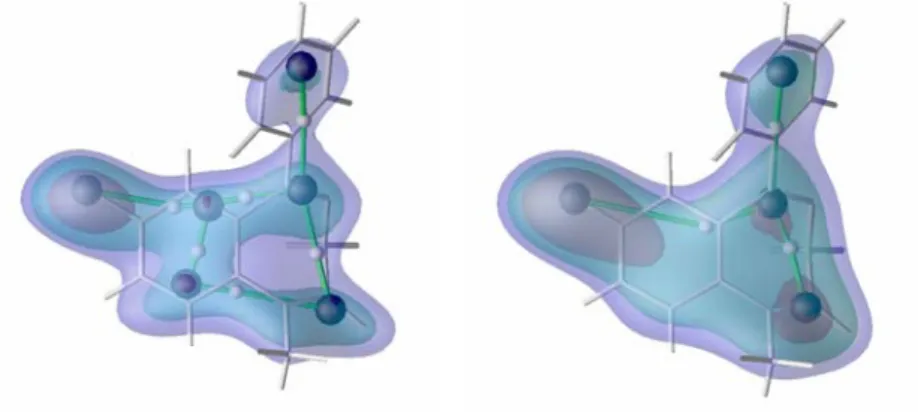
As announced hereabove, to maximize the interatomic distances between the backbone and side chain atoms, an extended geometry characterized by Ω = 180°, Φ = -139°, Ψ = 135° was considered. Indeed, for MEP analyses, the conformation of the peptide appeared to be extremely important on the results of the merging/clustering algorithm applied to MEP functions. This is illustrated in Figures III.1 and III.2 that respectively depict the smoothed ED and MEP obtained at t = 1.4 bohr2 for a β-strand and a α-helix of Gly15. As already established before [20,29], the ED-based

decomposition of the protein backbone is rather regular, consisting mainly in fragments (C=O)AA(N-Cα)AA+1.

Figure III.1. ED iso-contours (0.05, 0.10, 0.15 e-_/bohr3_{) of (top) β-Gly}

15 and (bottom) α-Gly15 smoothed at t = 1.4 bohr2.

Local maxima at t = 1.4 bohr2 _{were obtained using the hierarchical merging/clustering algorithm applied to the PASA}

ED distribution function. CG points are numbered as in Table III.III. Figures were generated using DataExplorer [47]. The dendrograms (Figure III.3) resulting from the application of our hierarchical merging/clustering algorithm shows that the ED-based merging of the atoms to form fragments first occurs between the H atoms and their chemically bonded neighbors at t = 0.05 bohr2. Then, as already shown [20,29], the C and O atoms of the backbone carbonyl groups begin to merge starting at t = 0.4 bohr2. From 0.65 to 0.9 bohr2, the atoms of the AA backbones merge until regular fragment structures such as (C=O)AA(N-Cα)AA+1 (H atoms are not mentioned for clarity) are fully

created at about t = 1.25 bohr2. At t = 1.4 bohr2, there still exists one peak per residue, and an rmsd value of 0.216 Å is observed between the coordinates of the backbone peaks and their corresponding c.o.m. (Figure III.4). A difference between the ED peaks of the α- and β-structures does not appear before t = 2.45 bohr2. At that smoothing level, the close packing of the residues that occurs in the helix structure leads to a faster reduction of the number of local ED maxima (Figure III.5). As just mentioned, at t = 1.4 bohr2, one observes one ED peak per residue, regardless of the secondary structure (Figures III.1 and III.3).

Figure III.2. MEP iso-contours (plain: -0.05, -0.03 ; grid: 0.03, 0.05 e-_{/bohr) of (top) β-Gly}

15 and (bottom) α-Gly15

smoothed at t = 1.4 bohr2_{. Local maxima and minima at t = 1.4 bohr}2 _{were obtained using the hierarchical}

merging/clustering algorithm applied to the all-atom Amber MEP function. CG points are numbered as in Table III.II. Figures were generated using DataExplorer [47].

When a MEP function is used, results differ from the ED-based ones, and are highly dependent on the backbone conformation. The dendrogram built from the results of the merging/clustering algorithm applied to the all-atom Amber MEP function illustrates that difference, and also shows that atoms are not necessarily merged according to their connectivity (Figure III.6). For example, at t = 1.4 bohr2, a value selected because the number of peaks/pits does not vary significantly any longer beyond that smoothing degree, the points that are close to the O and C atoms (Figure III.2) are the result from the merge of the atoms (O, N, Cα) and (H, C, Hα, Hα), respectively. For an easier identification of those points, the corresponding closest atom in the molecular structure is given in Table III.II. In the case of β-Gly15, one interestingly observes an

the dipolar character of the global structure is strongly emphasized with negative and positive charges being distributed at each end of the peptide, respectively (Figure III.2).

Figure III.3. Dendrogram depicting the results of the hierarchical merging/clustering algorithm applied to the PASA ED distribution function of β-Gly15. Results are displayed for the atoms of the first nine AA residues only. The vertical line

locates t = 1.4 bohr2_.

Corresponding charge values, q1.4, fitted from the MEP grids smoothed at t = 1.4 bohr2, are

presented in Table III.II. For β-Gly15, the sign of the charges correspond to the expected dipolar

distribution, i.e., a positive and negative net charge close to the C and O atoms, respectively. For α-Gly15, this expected charge distribution is observed only for residues 2, 4-7, and 15. It is thus

hardly transferable from one residue to another. There are also additional charges that are close to the N atoms, with charge values being either positive (e.g., point 15) or negative (e.g., point 18).

Table III.II. CG charges q1.4 andq0.0 (in e-) of Gly15 fitted from the all-atom Amber MEP grids smoothed at t = 1.4 and

0.0 bohr2_{, respectively, using the program QFIT. Local maxima and minima at t = 1.4 bohr}2 _{were obtained using the}

hierarchical merging/clustering algorithm applied to the all-atom Amber MEP function. For each point, the distance vs. the closest atom, d, is given in Å. rmsdV and rmsdμ are given in kcal/mol and D, respectively. Point numbers (#) refer to Figure III.2.

α-helix β-strand

# Closest atom d q1.4 q0.0 Closest atom d q1.4 q0.0

1 N Gly1 0.768 -0.042 -0.014 O Gly1 0.599 -0.329 -0.311 2 H Gly3 0.973 0.261 0.216 H Gly1 1.212 0.011 0.026 3 O Gly1 0.681 -0.002 -0.076 Hα Gly1 1.120 0.218 0.189 4 C Gly2 0.899 0.246 0.307 C Gly2 0.797 0.261 0.256 5 O Gly2 0.598 -0.139 -0.187 O Gly2 0.605 -0.241 -0.236 6 O Gly3 0.560 -0.024 -0.074 C Gly3 0.840 0.201 0.214 7 C Gly4 0.771 0.290 0.307 O Gly3 0.624 -0.184 -0.205 8 O Gly4 0.524 -0.325 -0.298 C Gly4 0.825 0.169 0.193 9 C Gly5 0.682 0.034 0.162 O Gly4 0.620 -0.187 -0.204 10 O Gly5 0.507 -0.038 -0.176 C Gly5 0.832 0.202 0.209 11 C Gly6 0.700 0.039 0.146 O Gly5 0.623 -0.191 -0.202 12 O Gly6 0.499 -0.027 -0.174 C Gly6 0.827 0.195 0.202 13 C Gly7 0.706 0.107 0.170 O Gly6 0.622 -0.197 -0.204 14 O Gly7 0.492 -0.088 -0.186 C Gly7 0.830 0.199 0.206 15 N Gly8 0.700 0.138 0.088 O Gly7 0.623 -0.197 -0.205 16 C Gly8 0.693 0.081 0.148 C Gly8 0.828 0.197 0.205 17 O Gly8 0.491 -0.110 -0.189 O Gly8 0.623 -0.196 -0.205 18 N Gly9 0.695 -0.024 0.030 C Gly9 0.829 0.198 0.208 19 C Gly9 0.698 0.048 0.131 O Gly9 0.623 -0.196 -0.205 20 N Gly10 0.691 0.005 0.066 C Gly10 0.828 0.194 0.203 21 O Gly9 0.499 -0.036 -0.138 O Gly10 0.623 -0.195 -0.204 22 C Gly10 0.716 -0.077 0.043 C Gly11 0.829 0.204 0.210 23 O Gly10 0.499 0.107 -0.001 O Gly11 0.623 -0.194 -0.204 24 N Gly11 0.675 0.005 0.039 C Gly12 0.828 0.180 0.196 25 C Gly11 0.747 -0.001 0.098 O Gly12 0.623 -0.197 -0.206 26 O Gly11 0.483 0.043 -0.050 C Gly13 0.830 0.219 0.221 27 N Gly12 0.678 -0.039 -0.019 O Gly13 0.626 -0.194 -0.205 28 C Gly12 0.824 0.186 0.209 C Gly14 0.823 0.207 0.212 29 O Gly12 0.581 -0.259 -0.252 O Gly14 0.633 -0.211 -0.213 30 O Gly13 0.619 -0.152 -0.144 C Gly15 0.608 0.275 0.273 31 O Gly14 0.619 -0.168 -0.159 O Gly15 0.762 -0.205 -0.200 32 C Gly15 0.587 0.242 0.242 33 O Gly15 0.648 -0.266 -0.250 rmsdV 1.12 1.85 0.67 1.32 rmsdμ 0.46 0.11 0.19 0.34