HAL Id: hal-01890387
https://hal.archives-ouvertes.fr/hal-01890387
Submitted on 4 Dec 2019
HAL is a multi-disciplinary open access
archive for the deposit and dissemination of
sci-entific research documents, whether they are
pub-lished or not. The documents may come from
teaching and research institutions in France or
abroad, or from public or private research centers.
L’archive ouverte pluridisciplinaire HAL, est
destinée au dépôt et à la diffusion de documents
scientifiques de niveau recherche, publiés ou non,
émanant des établissements d’enseignement et de
recherche français ou étrangers, des laboratoires
publics ou privés.
slurry intensified continuous chemical reactor
Sami Bahroun, S. Li, Christian Jallut, Claire Valentin, F. De Panthou
To cite this version:
Sami Bahroun, S. Li, Christian Jallut, Claire Valentin, F. De Panthou. Control and optimization
of a three-phase catalytic slurry intensified continuous chemical reactor. Journal of Process Control,
Elsevier, 2010, 20 (5), pp.664-675. �10.1016/j.jprocont.2010.03.002�. �hal-01890387�
Control and optimization of a three-phase catalytic slurry
intensified continuous chemical reactor
S. Bahroun1,*, S. Li1, C. Jallut1, C. Valentin1, F. De Panthou2
1 Université de Lyon, F-69622, Lyon, France;
Université Lyon 1, Villeurbanne; LAGEP, UMR 5007, CNRS, CPE, 43, Bd du 11 Novembre 1918, 69100 Villeurbanne cedex, France;
2 AETGROUP SAS, 6 montée du Coteau, 06800 Cagnes-sur-mer, France,
(E-mail: fabrice.depanthou@aetgroup.com, Tel: (+33)6 24 05 25 83, Fax: (+33)4 92 08 53 40).
*Corresponding author: Sami Bahroun
(E-mail: bahroun@lagep.univ-lyon1.fr, Tel: (+33)4 72 43 18 81, Fax: (+33)4 72 43 18 99). Abstract: Intensified continuous mini-reactors working in high pressure and temperature conditions are particularly effective at coping with mass transfer limitations during three-phase catalytic reactions. They are highly non-linear, multivariable systems and behave differently from conventional batch, fed-batch or continuous non-intensified reactors. In this paper, the optimization and control of this new process are presented using a two-layer approach consisting of a hierarchical control structure with an optimization layer which calculates the set points for an advanced controller. The latter is based on the concavity of the entropy function and the use of thermodynamic availability as a Lyapunov function. The three-phase catalytic o-cresol hydrogenation performed under high pressure and temperature in a small-scale pilot of the RAPTOR® reactor designed by the French company AETGROUP SAS, is taken as a representative test example to illustrate the strategy. The performance of the control structure is illustrated by simulation.
Keywords: Lyapunov based control; Dynamic modeling; Three-phase catalytic reaction; Intensified continuous reactor; Entropy based control.
1. Introduction
Although the batch reactor remains a key tool in the field of fine chemicals and pharmaceuticals due to its high flexibility and versatility, it presents a number of technological limitations, in particular, poor transfer of the heat released by exothermic chemical reactions and the required use of solvents which creates serious problems with regard to safety [1].
For some years, an alternative to batch reactors has been developed, thanks to progress in process intensification and the development of intensified continuous mini-reactors [2][3]. The intensification leads to the improved control of heat and mass transfer that makes it possible to concentrate the reagent and thus limit the quantities of solvent to be treated, as well as the inventory of hazardous substances. Consequently, the intensified continuous chemical reactors seem to be inherently safer than
the conventional batch reactors, but the issue of their control has been raised by some authors [4] as these reactors are smaller and more sensitive to disturbances and they are required to work under high pressure and temperature conditions.
This paper deals with the modeling and control of an intensified continuous stirred mini-reactor, the “RAPTOR®” (French acronym for “Réacteur Agité Polyvalent à Transfert Optimisé Rectiligne” or “Polyvalent Rectilinear Stirred Reactor With Optimized Transfer”), recently developed by AETGROUP SAS Company, a French company whose main activity is chemical process industrialization and continuous process technology. This reactor is particularly good at coping with mass transfer limitations during three-phase catalytic reactions due to its highly efficient stirring system. It is also well adapted to process intensification under extreme pressure and temperature conditions (up to 300°C and 250 bar) making it possible for a complete reaction to take place with just a few minutes residence time. In terms of catalytic reactions, this reactor can handle dispersed catalyst. For reasons of confidentiality, a detailed description of the RAPTOR® cannot be given. The case of a three-phase catalytic hydrogenation reaction is taken as a representative test example. The aim of this paper is to describe control law synthesis for intensified three-phase continuous reactors that find their basis in irreversible thermodynamics. This choice has been made due to the specific energetic features of the intensified continuous mini-reactors that will be detailed below.
As far as the control of chemical reactors is concerned, many general studies concerning the control of homogeneous chemical processes have been published. Traditional control techniques using linear system analysis and design tools together with linearized models have been used [5-7]. A stabilization of a class of continuous stirred tank reactors (CSTR) under classical PI control with temperature feedback was proposed by Alvarez-Ramirez and Morales [11]. However the use of these techniques is limited since chemical processes are highly non-linear. Therefore different non-linear methods have been proposed to control homogeneous chemical processes [48] [49]. Feedback linearization techniques have been proposed by Limqueco and Kantor in [8], where a non-linear output feedback controller is built for an exothermic, first-order reaction. Input – Output linearizing control was used by Kravaris and Chung [9]to design a control law for trajectory tracking in batch reactor. Dochain [10] developed an input-output linearizing adaptive controller to control the temperature in non-isothermal stirred-tank reactor. Non-linear geometric control tools have been used in Alvarez-Ramirez [12] and Alvarez-Ramirez, Suarez and Femat [13], to stabilize unstable steady states in CSTR. An Interconnection and Damping Assignment-Passivity Based Control (IDA-PBC) approach was proposed by Ramírez in [14] for the control of a non-minimum phase Multi-Input Multi-Output (MIMO) CSTR. Lyapunov based control was used by Antonellia [15] to design non-linear output feedback control for the temperature stabilization of a CSTR, in the presence of input constraints and uncertainty in the kinetic parameters. Applications of sliding mode controllers to chemical processes [16] [17] have also attracted significant interest. In Chen [17], simulation results revealed that the proposed sliding mode control system design methodology is applicable and promising for the non-linear regulation of time-delay chemical processes.
Some research has been devoted to the control of non-intensified continuous three-phase catalytic hydrogenation reactors. Rezende et al. [27] and Delba Melo et al. [28] evaluated a two-layer approach for the control of a three-phase catalytic reactor. It consists of an optimization layer that calculates the set points and manipulated variables to the advanced controller layer. The controller used was a multivariable predictive controller based on the Dynamic Matrix Control approach (DMC) in [27] and on the Quadratic Dynamic Matrix Control approach (QDMC) in [28]. The problem of optimization was solved by using the Successive Quadratic Programming (SQP) algorithm in [27] and the Levenberg–Marquardt and SQP method as the optimization algorithm in [28]. Rezende et al. [29] proposed a one-layer approach to control a three-phase catalytic reactor. The predictive DMC was used as the process controller, the optimization problem being solved by the using the Genetic Algorithm. Delba Melo et al. [30] assessed the performance of different control strategies in a three-phase catalytic reactor: feedback control, feedforward control and a combination of both strategies. The feedback strategy was implemented by using the predictive QDMC. The feedforward action was calculated with the aim of minimizing a quadratic error between the calculated exit reactor temperature and the set-point for this process variable.
By analyzing these different approaches, we can see that they involve general mathematical and control tools, and do not take energy and thermodynamic considerations into account. Looking at the problem from a different angle, our goal is to synthesize entropy based control laws based on irreversible thermodynamics. The link between thermodynamics and control strategy started with Warden, Aris and Amundson [18], who carried out stability analysis of CSTR for finite disturbances, and Dammer and Tells [19] who studied open reaction systems with stable and unstable steady states far from thermodynamic equilibrium. Georgakis [20] proposed a non-linear control structure that is based on extensive thermodynamic variables. In [21], Favache and Dochain presented an extension of Georgakis’s results [20] regarding the stability analysis of the CSTR. They proposed different candidate Lyapunov functions related to thermodynamic and based specifically on the entropy, the entropy production and the internal energy. Alonzo and Ydstie combined thermodynamic, passivity and Lyapunov theory. The basis of this theory was established by Ydstie and Alonzo [22][23] in the context of passive control design and the control of distributed systems in [24], and transport reaction systems in Ruszkowski and Ydstie [25].
This paper deals with the dynamic modeling and control of a significantly complex situation as it studies the case of a three-phase catalytic hydrogenation reaction performed in an intensified continuous chemical reactor. Analyzing the design, control and safety of this type of reactors is important for the future of the fine chemicals industry. Such processes involve complex reactions with constraints on thermal stability and/or selectivity [2]. The dynamic modeling of these reactors is also more difficult since three phases are involved in the process. These three phases are mobile and exchange species and energy. Moreover, the chemical reactions that take place are highly exothermic. The resulting process is then a multivariable highly non-linear system.
In the present work, a two-layer control approach was developed for the control of the jacketed continuous intensified reactor “RAPTOR®”, with the aim of rejecting disturbances whilst maintaining safety. The choice of the controlled, manipulated and measured variables was guided by conventional industrial practices. The aim was to control the conversion at the reactor outlet. As the conversion cannot be measured online or only using a very expensive sensor, the controlled variable chosen was temperature at the mini-reactor outlet, which can be easily measured online. This point is discussed in section 4. The manipulated variable is the inlet jacket temperature, as for most of the industrial applications. The measured variables are the outlet fluid temperature and the reactor body temperature, both of which can be easily measured in an industrial context. Constraints on the highest admissible temperature for the metal body reactor, as well as the dynamic behavior of the manipulated variable must be taken into account. The resolution of an optimization problem is combined with an advanced control algorithm based on irreversible thermodynamics. This approach is based on the works of Alonso [22], Ydstie [23], Ruszkowski [25] and Hoang [31] [32]. O-cresol hydrogenation to obtain 2-methyl-cyclohexanol is taken as an example to illustrate the approach through simulations obtained from a mathematical dynamic model of the system. The finite dimension dynamic model that we propose consists of mass and energy balance equations for the catalyst particles the gas phase and the liquid bulk phase, and is based on a spatial discretization of the reactor. The transient heat transfer between the metal body of the reactor, the coolant fluid and the bulk fluid is also taken into account due to the high (reactor body mass)/(bulk mass) ratio that is a common feature of intensified reactors [33].
2. Dynamic behavior of the continuous mini-reactor
2.1 Model principle
Developing efficient and reliable dynamic models for three-phase catalytic slurry continuous reactors is still a difficult task because it involves many aspects including hydrodynamics, gas-liquid and liquid-solid mass transfer, heat transfer, and reaction kinetics [34]. The extreme pressure and temperature conditions and the highly efficient stirring in the RAPTOR®, make it necessary to model all these aspects because the reaction is no longer limited by mass transfer. In the literature, we find studies proposing the dynamic modeling and control of catalytic three-phase reactors [26][35-39] but as far as we know, the problem of intensified continuous mini-reactors modeling has not been addressed.
The model presented here describes the dynamic behavior of the intensified continuous mini-reactor during the catalytic hydrogenation of o-cresol. In this case, hydrogen reacts with o-cresol without solvent due to the high heat and mass transfer capacities of the mini-reactor. A three-phase catalytic reactor is a system in which gas and liquid phases are brought into
contact with a porous solid phase. The reaction occurs between a dissolved gas and a liquid-phase reactant in presence of a catalyst deposited on the surface of the porous solid support [40] according to the following global stoichiometric equation:
A(g) +
ν
BB(l) →ν
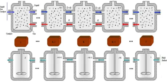
CC(l) (1)Due to the presence of the efficient stirrer and the tubular nature of the reactor, bulk flow through the mini-reactor is treated as an association of J perfectly mixed reactors (CSTR) in series with back mixing effect as is typical for chemical reactor modeling (see Fig. 1). This is a method for the spatial discretization of the flow that is an infinite dimension system at the beginning. This flow arrangement makes it possible to take into account axial mixing within the reactor and has been confirmed by RTD measurements. It is presumed to hold for the three phases. Similarly, the counter current flow through the jacket is treated as an association of J perfectly stirred tank reactors in series. This means of considering the flows in the reactor and in the jacket is highly flexible and leads to a finite dimension model [41].
1 K-1 K K+1 J
1 K-1 K K+1 J
1 K-1 K K+1 J
Fig. 1. Flow model and spatial discretization of the mini-reactor.
A specificity of an intensified continuous mini-reactor is the large size of the metal body in relation to the volume of fluid which allows it to withstand high pressure and temperature. Therefore, the influence of the reactor body itself may be significant with respect to the thermal transient behavior of the system [33]. Consequently, the body of the mini-reactor is broken down into J pieces with uniform temperatures (see Fig. 1) in order to include a description of the reactor body in the model.
2.2 Dynamic model equations
The model consists of mass and energy balance equations for the catalyst particles, the gas phase and liquid-bulk phase, and also energy balance equations for the body of the reactor and for the cooling fluid flowing through the jacket [42].
In three-phase catalytic reactions, the reaction rate is calculated by using the Langmuir-Hinshelwood model [43]:
R
=
k
K
AK
BC
AsC
Bs1
+
K
AC
As(
)
(
1
+
K
BC
Bs)
(2)where A stands for hydrogen, B for o-cresol, C for 2-methylcyclohexanol. CAs and CBs are respectively the hydrogen and
o-cresol concentrations within the catalyst pores that are presumed to be uniform within the catalyst pellets.
The variations of the rate constant k with temperature are given by the Arrhenius law while those of the adsorption constants
KA and KB are derived from the mass action law [43]:
k=5,46.108exp(−82220 / RT
s) (3)
KA=10,55.10−3exp(+5003/RTs) (4)
KB=7,54.10−6exp(+16325/RTs) (5)
where Ts is the catalyst pellet temperature that is presumed to be uniform. The parameters KA and KB in equations (4) and (5)
are adsorption equilibrium constants that decrease with temperature. These parameters are involved in the Langmuir – Hinshelwood mechanism that includes adsorption elementary steps.
The following assumptions are considered to derive the model [26] [38] [42]:
• the temperature of the liquid and gaseous phases is considered to be equal;
• a global mass transfer coefficient is used to represent hydrogen transfer from the liquid surface to the bulk. Equilibrium conditions at the gas-liquid interface are assumed;
• the pressure drop is negligible;
• the resistances to mass and heat transfer at the catalyst pellet surface and within the pores are lumped into the overall heat and mass transfer coefficients;
• the material balance in the gas phase, assumed to be pure hydrogen, is given as a steady state;
• the gaseous phase is assumed to be ideal.
Let us first consider the dynamic part of the model. The balance equations are written for each set of three elementary volumes, the bulkVk, the jacket cooling liquid Vjk and the reactor metal body Vmk , denoted by the k index (see Fig. 1). The bulk volume is made up of three phases: the liquid phase volume is εlkV
( + + k =1
g k l s
ε
ε
ε
). The gaseous phase hold-upε
gk and therefore the gas-liquid interface specific areaa
glk are assumed to varyalong the reactor axis due to hydrogen consumption. Consequently, the gaseous phase volumetric flow rate varies with the k index whilst the volumetric flow rates of the liquid and solid phases ql and qs are assumed to be constant.
Mass balance of reactant A
liquid phase
( )
(
)
(
)
(
k)
Al k Al k k k As k Al ls lsA k k Al l k Al l k Al l k Al k k lV dCdt =1+αqC−1+αqC+1−1+2αqC −Vk a C −C +VkglaglC* −C ε (6) solid phase( )
1 s Ask1 s Ask1(
1 2)
s Ask k lsA ls(
Alk Ask)
A s s k ( Ask, Bsk, sk) k As k sV dCdt αqC αqC αqC Vk a C C ν ερVRC C T ε = + − + + − + + − − (7)The hydrogen solubility at the gas-liquid interface is calculated by using the Henry constant that is available in [43]:
= = k f k *k Al RT P He P C 4990 exp 11538 (8)
Mass balance of reactant B
liquid phase ) ( ) 2 1 ( ) 1 ( 1 1 k Bs k Bl ls lsB k k Bl l k Bl l k Bl l k Bl k k lV dCdt = +α q C − +αq C + − + α q C −V k a C −C ε (9) solid phase
( )
(
)
(
)
(
k)
s k Bs k As k s s B k Bs k Bl ls lsB k k Bs s k Bs s k Bs s k Bs k sV dCdt 1 αqC 1 αqC 1 1 2αqC Vk a C C ν ε ρVRC ,C ,T ε = + −+ + − + + − − (10) Energy balancesfluid (gas and liquid) phases
(
)
(
)
(
)
(
k)
f l k f l k f l pl l k f k g k f k g k f k g pg g k f k s ls s k k f k m k k f pl l k l pg g k g k T q T q T q C T q T q T q C T T a h V T T hS dt dT C C V ) 2 1 ( ) 1 ( ) 2 1 ( ) 1 ( ) ( 1 1 1 1 1 1 α α α ρ α α α ρ ρ ε ρ ε + − + + + + − + + + − + − = + + − + + − − (11) solid phase(
)
(
( )
(
) (
)
)
(
k)
s k s B k s A r s k s k s k s s k s k s s ps s k s k f ls s k k s ps s k sVρC dTdt =Vha T −T −ρC 1+αq T −T −1 +αq T −T +1 −εVρ∆ HRC,,C ,,T ε (12)mini-reactor metal body
(
)
(
k)
m k J j k j k m k f k k m pm m mk C dTdt hS T T h S T T V ρ = − + − +1− (13) cooling medium(
− +1 −)
−(
− −1)
= k j k j j pj j k j k J m k j k j pj j jk dt h S T T C q T T dT C V ρ ρ (14)In order to take into account gaseous phase hydrogen consumption, the steady-state hydrogen mass balance is given according to equation (15):
(
1+2α)
εgkSTJAg+Vkkglakgl(
CkAl*−CAlk)
=(
1+α)
εgk−1STJAg+αεgk+1STJAg (15) The hydrogen consumption is assumed to only reduce the gas hold-upε
gk in equation (15) which means that the hydrogen fluxJAg is assumed to be constant. The number of spherical bubblesNbk, with a constant radiusrb, represents the gas hold-up
ε
gkaccording to the equation (16).
3 3 4 b k b k k gV N
π
rε
= (16)The gas-liquid interface surface area aglk depends on the number of spherical bubblesNbk according to the equation (17).
2
4
b k b k k glV
N
r
a
=
π
(17)The gas hold-up
ε
gk and fluid hold-upε
lk are linked by the equation (18). 1 = + + k g k l sε
ε
ε
(18)To summarize, the algebro-differential finite dimension dynamic model of the elementary kth CSTR has 9 state variables:
k g k J j k m k f k s k Bs k Bl k As k Al
C
C
C
T
T
T
T
C
,
,
,
,
,
,
,
−+1,
ε
. The 9 independent equations are the 8 dynamic balance equations (6), (7), (9),(10), (11), (12), (13) and (14), and the gas phase steady-state balance equation (15). To solve this algebro-differential equations system, 8 constitutive equations (2), (3), (4), (5), (8), (16), (17) and (18) are used to express
R,k,K
A,K
B,ε
lk,C
Al*k,N
bk,a
glk.2.3 Open loop simulation results for consistency and sensitivity analysis
The mathematical dynamic model that we developed makes it possible to reproduce the main features of the open-loop dynamic behavior of the intensified continuous mini-reactor. The nominal operating point of a small-scale pilot of the RAPTOR® is defined as follows. A slurry made of catalyst dispersed in liquid o-cresol is fed into the reactor with hydrogen at 200 bar. The cooling medium jacket inlet temperature is Tj0. The inlet gaseous phase hold-up is 47.5%. The main parameters
used for the simulation are given in table 1. In Fig. 2, the trajectory toward the steady state of the reactor as soon as the hydrogen is introduced is represented by the dynamic behavior of the reactor outlet temperature variation from initial conditions. The operating conditions lead to a reference steady-state o-cresol conversion in the liquid phase of up to 98% at the reactor outlet, which is a very good industrial target. We observe that the fluid temperature is limited and increases by 102°C. The catalyst temperature is slightly higher than that of the reactant fluid since the reaction takes place within the catalyst pores. We also observe that the jacket temperature remains nearly constant which is due to the high value of the cooling fluid flow rate in the jacket compared to the fluid flow rate inside the reactor which quickly removes heat from the reactor body. The temperature of the reactor body increases by only 63°C.
Process variable P V ∆rH KlsAals KlsBals Cps ρs Cpm hsals Numerical Value 200 x 105 Pa 2.4 x 10⁻³ m3 -200 x 103 J. mol-1 5.6 s-1 3 s-1 150 J. kg-1. K-1 1547 kg. m-3 500 J. kg-1. K-1 20 x 105 W. m-3.K-1 Table1: Parameters used for simulation
The metal body plays the same role as the one of a solvent in the case of a batch or fed-batch reactor. This behavior has been well documented in the literature [33]. The accumulation capacity acts only during transient periods. Such transient periods are those occurring after an incident. The reactor body tends to accumulate the energy released by the reaction thanks to its high mass compared to the bulk phases inventory mass ((reactor body mass / bulk mass) > 10).
0 200 400 600 800 1000 1200 1400 1600 1800 2000 0 20 40 60 80 100 120 Time (s) T e m p e ra tu re v a ri a ti o n ( °C ) Catalyst Temperature Fluid Temperature Metal Temperature Jacket Temperature
Fig. 2. Dynamic behavior of the intensified continuous mini-reactor outlet temperatures.
We also provide some results from steady-state simulations in order to check the model’s consistency, as well as the model output sensitivity analysis with respect to input and disturbances (for confidentiality reasons, only differences with respect to values obtained for the reference steady state are presented).
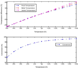
-5% -4% -3% -2% -1% Tjo +1% +2% +3% +4% +5% -20 -10 0 10 20 T e m p e ra tu re d if fe re n c e ( °C ) Temperature (K) -5% -4% -3% -2% -1% Tjo +1% +2% +3% +4% +5% 90 92 94 96 98 100 C o n v e rs io n ( % ) Temperature (K) Fluid Temperature Metal Temperature Jacket Temperature Conversion
As far as intensified continuous reactors are concerned, the reaction takes place at a very high temperature and the jacket plays a dual role in the evolution of the reaction. On the one hand, it makes it possible to obtain good outlet conversion by increasing the temperature of the bulk. On the other hand, it affects safety since the jacket fluid makes it possible to cool the temperature of the bulk in order to avoid thermal runaway. A suitable compromise must be found.
Fig. 3 illustrates the steady-state characterization of outlet bulk temperature and conversion with respect to the inlet jacket temperature. From this figure, it is observed that both outlet bulk temperature and conversion are very sensitive to the inlet temperature of the jacket fluid.
We will now consider the effects of small changes that can occur in the operating conditions which are considered as disturbances. Only those leading to the widest variations in the system’s steady state are presented here.
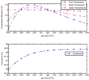
-30%-2 -25% -20% -15% -10% -5% qg0 +5% +10% +15% +20% +25% +30% -1.5 -1 -0.5 0 0.5 T e m p e ra tu re d if fe re n c e ( °C ) gas flow (m3/s) -30% -25% -20% -15% -10% -5% qg0 +5% +10% +15% +20% +25% +30% 95.5 96 96.5 97 97.5 98 98.5 99 C o n v e rs io n ( % ) gas flow (m3/s) Fluid Temperature Metal Temperature Jacket Temperature Conversion
Fig. 4. Steady state characterization of bulk outlet temperature and conversion with respect to inlet gas flow qg0.
Fig. 4 illustrates the steady state characterization of outlet bulk temperature and conversion with respect to inlet gas flow. This figure highlights the fact that outlet conversion is more sensitive to variations on qg0 than outlet temperature, whilst there is a
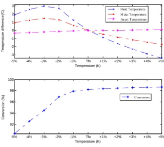
-5% -4% -3% -2% -1% Tfo +1% +2% +3% +4% +5% -3 -2 -1 0 1 2 3 T em p er a tur e d if fe ren c e( °C ) Temperature (K) -5% -4% -3% -2% -1% Tfo +1% +2% +3% +4% +5% 92 94 96 98 100 C o nv e rs io n ( % ) Temperature (K) Fluid Temperature Metal Temperature Jacket Temperature Conversion
Fig. 5. Steady state characterization of bulk outlet temperature and conversion with respect to inlet fluid temperature Tf0.
-30% -25% -20% -15% -10% -5% qlo +5% +10% +15% +20% +25% +30% -60 -40 -20 0 20 T e m p e ra tu re d if fe re n c e ( °C ) Volume flow (m3/s) -30% -25% -20% -15% -10% -5% qlo +5% +10% +15% +20% +25% +30% 80 85 90 95 100 C o n v e rs io n ( % ) Volume flow (m3/s) Fluid Temperature Metal Temperature Jacket Temperature Conversion
Fig. 6. Steady state characterization of bulk outlet temperature and conversion with respect to inlet volume flow ql0.
Fig. 5 shows the effect of inlet bulk fluid temperature on the behavior of outlet bulk temperature and conversion. This figure points out that only conversion is sensitive to the variations of Tf0. As a result, a disturbance to inlet fluid temperature greatly
affects the quality of the outlet product.
In Fig. 6, the steady state characterization of bulk outlet temperature and conversion with respect to inlet bulk fluid flow is highlighted. We note that both the bulk outlet temperature and conversion are highly sensitive to ql0. In fact, a 30% decrease in
the inlet bulk fluid flow rate makes it possible to obtain total conversion with improved thermal conditions. However this result leads to a lower production rate and is therefore of less interest.
According to the observations shown in Fig. 3 to Fig. 6, the conversion is very sensitive to variations in inlet gas flow rate, inlet bulk fluid flow rate and temperature, so a disturbance in these variables greatly affects the quality of the outlet product and possibly the safety conditions. As the output variables are very sensitive to the inlet jacket temperature Tj0, we can
conclude that this variable may be chosen as an effective manipulated variable in accordance with industrial practice.
Having examined the open loop considerations, we will now discuss how a control structure based on irreversible thermodynamics can be synthesized. The goal is to regulate conversion whilst avoiding thermal runaways. Therefore, methods for implementing stabilizing control are of interest and involve searching for a candidate Lyapunov function related to some of the energetic features of the reactor under consideration.
3. Thermodynamics aspect and availability function
In this section, we briefly summarize how a Lyapunov function for thermodynamic systems, the availability function, can be built. The availability function is issued from the second law of thermodynamics. It is positive for thermodynamic systems that are assumed to remain homogeneous. Its construction is based on two fundamental concepts of thermodynamics.
On the one hand, one has to consider the way the entropy S of a homogeneous mixture can be expressed according to the Gibbs equation [47]: dS= 1 T dU+ P T dV− µi T dNi i=1 I
∑
(19)U and V are the internal energy and the volume of the system, T, P its temperature and pressure, µi the chemical potential and
Ni the number of moles of component i.
On the other hand, the second law of thermodynamics makes it possible to derive some constraints that the entropy of a homogeneous phase should satisfy. As a matter of fact, the entropy balance for an isolated system is:
dS
dt =σ ≥0 (20)
The equation (20) gives phase stability conditions of an equilibrium point for an isolated system since any trajectory that would lead to a destruction of entropy is impossible according to the second law [44][47]. Conversely, a condition that should satisfy any thermodynamic model that is used to calculate S from equation (19) in any conditions can be derived from equation (20) if the system under consideration is assumed to remain homogeneous. This condition is that the entropy function S=S U,V ,N
(
i)
entropy surface at this equilibrium point. This condition is also valid for an open system that is not at equilibrium according to the so-called local equilibrium principle. Consequently, it can be applied to the steady state of a chemical process.
The way to apply this condition consists in defining a distance between the tangent plane to the entropy surface and the entropy function. For small deviations from equilibrium or steady-state points, the so-called
δ
2S<0 function has been defined tocharacterize the local curvature of the entropy function and used by the Brussels School of Thermodynamic [44], [46]. In the case of major disturbances, a finite distance between the tangent plane and the entropy function can be considered that reduces to
−
δ
2S
>
0
for small disturbances. Since the entropy function S=S U,V ,N(
i)
is a first order homogeneous function, that is tosay the Euler theorem applies [53][54]:
∑
= − + = I i i i N T V T P U T S 1 1 µ (21)it can be easily verified that the following expression is valid:
(
)
(
)
(
) (
)
(
)
∑
∑
− − − + − + − − − + − + = I i i i i I i i i i i i T T N T P T P V T T U N N T V V T P U U T N V U S N V U S µ µ µ 1 1 1 , , , , (22)where the overbar stands for the steady-state point under consideration. The quantity
(
) (
+ −) (
+ −)
−∑
I(
−)
i i i i i T U U TP V V T N N N V US , , 1 µ is the equation of the tangent plane to the entropy surface at the point
(
U ,
,
V
N
i)
since: T N S T P V S T U S i i µ ∂ ∂ ∂ ∂ ∂ ∂ − = = = 1(23)
from equation (19). Then the condition:
0 1 1 > − − − + − =
∑
I i i i i T T N T P T P V T T U A µ µ (24)must be satisfied for the homogeneous phase to be stable. This quantity has been defined as the availability
A
within the context of process control by Ydstie and co-workers [22-25] and recently applied to the non-isothermal CSTR stabilization [31][32]. In order to use the availability concept according to this approach, its time derivative dAdt has to be calculated and the
way the condition A=0 is satisfied must be analyzed. As a matter of fact, S=S U,V ,N
(
i)
is not strictly concave, thus thecondition A=0 is not only verified for the steady-state point under consideration but also for all the points U
(
k,Vk,Ni,k)
satisfying the conditions (see equation (24)):T
(
λU ,λV ,λN i)
=T U ,V ,N(
i)
P(
λU ,λV ,λN i)
=P U ,V ,N(
i)
µi
(
λU ,λV ,λN i)
=µi(
U ,V ,N i)
(25)
since T U,V,N
(
i)
, P U,V ,N(
i)
and µi(
U,V,Ni)
are zero order homogeneous functions with respect to(
U,V,Ni)
. In order for the entropy to be strictly concave and the condition A=0 to be satisfied only at the steady-state point under consideration, a constraint has to be imposed on the system, specifically on at least one extensive variable.4. Proposition for a new industrially applicable control structure
4.1 Principle
The choice of the intensified continuous mini-reactor control strategy depends on operational objectives such as safe operation, high product quality, energy savings, environmental constraints or economic gain [4][27][50][51].The two main objectives of the controller are a high conversion rate of the reactant and safe operation. The latter is obtained if the reactor’s metal body temperature does not exceed a maximum denotedTmmax. Furthermore, the controller has to reject measured disturbances – i.e. - the inlet gas flow qg0, the inlet bulk fluid temperature Tf0 and the inlet bulk fluid flow ql0. As the conversion cannot be measured
online, or only by means of a very expensive sensor, an indirect way of controlling the outlet conversion is to control outlet bulk temperature, which can be easily measured. Such indirect control can be obtained by controlling the temperature of the metal body at the outlet i.e. - TmJ (see Fig.1) since the metal body of the reactor is very large when compared to the bulk phases inventory mass. As a matter of fact, the reactor body tends to accumulate the energy released by the reaction. This characteristic of the intensified reactors has been shown to improve their inherent safety [33]. The variable TmJ is also easily measurable in an industrial context. These specific energetic features of the mini-reactor are well-suited to designing a control law based on thermodynamic concepts such as the availability used as a Lyapunov function.
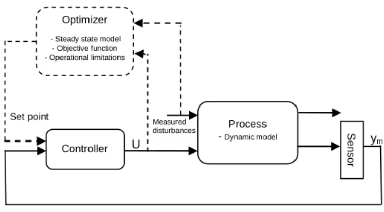
The controller that we propose is based on a two-layer hierarchical approach with an upper optimization layer and an advanced control layer, as presented in Fig. 7. The proposed control law is based on measurements which can be easily obtained in industrial conditions: the outlet bulk fluid temperature TfJand the reactor body temperature J
m
T at the outlet axial position as well as the disturbances (the inlet gas flow qg0, the inlet bulk fluid temperature Tf0 and the inlet bulk fluid flow ql0). Figure 3
pointed out that the choice of the inlet jacket temperature, 0 j
T , as a manipulated variable, according to industrial practice, is
very relevant. Process - Dynamic model Controller U Measured disturbances Set point Optimizer - Steady state model
- Objective function - Operational limitations S e n so r ym
Fig. 7. The two-layer hierarchical control approach.
This hierarchical control scheme is validated by numerical simulation. Thus, the process block is composed of the dynamic model presented in section 2 (equations (2) to (18)). The corresponding steady-state model is used in the optimizer block that also includes the operational limitations (the materials used for the gaskets impose a constraint on the temperature of the intensified reactor’s metal body atTmmax) and the objective function (desired o-cresol conversion in the outlet bulk phase,
0 0 Bl Bl Bl C C C − =
η ). The controller block includes an advanced controller based on availability as a Lyapunov function.
4.2 Inner loop entropy-based controller synthesis
During each sample period,tk-1
<
t<
tk, the optimization layer calculates a constant set point TmkJ of the reactor’s metal bodytemperature at the outlet axial position (see Fig 1). J mk
T is an input for the inner loop output feedback controller. This controller calculates the input 0 ,
j
T to apply during the inner loop control horizon. The inner loop control law proposed in this paper is
a Lyapunov function. As the mass of the bulk inventory is very low when compared to the mass of the intensified reactor’s metal body, one can assume that A≈Am where A and Am are respectively the availability of the mini-reactor and its content and that of its metal body. The metal body of the reactor is homogeneous so its availability can therefore be calculated. Furthermore, the mass and the volume of this metal body are constant so its entropy can be considered as strictly concave. The availability of the metal body associated to the Jth CSTR with respect to J
m T is: 0 1 1 > − − − + − = J m J m J m J m J m J m J m J m J m J m J m J m T T U TP TP V N T T A
µ
µ
(26)The output feedback control is designed so that mJ <0
dt
dA during the control horizon
1 + k k<t<t t . Since J m N and J m V are constant, the time derivative of AmJ is given as:
dAmJ dt = 1 T mJ −T1 mJ dUm J dt (27)
The energy balance for the reactor body associated to the JTh CSTR can be given as follows:
) ( ) ( 0 J m j k j J m J f k J m hS T T hS T T dt dU = − + − (28)
From equations (27) and (28), the dynamic equation for J m A is:
dA
mJdt
=
1
T
mJ−
1
T
mJ
(
hS
kT
fJ−
(
hS
k+
h
jS
k)
T
mJ+
h
jS
kT
j0)
(29)Let us choose the following non-linear control law expressed as a function of measured state variables:
(
)
− − + + − = J m J m c J m k j k J f k k j j T T K T S h hS T hS S h T0 1 1 1 (30)with Kc strictly positive, so that <0
dt dAJ m . Then: 2 1 1 − − = J m J m c J m T T K dt dA (31)
A very similar stabilizing control law has been obtained by Hoang et al. [31][55] for the non isothermal CSTR by separating the total availability of the bulk into thermal availability and material availability and by designing a control law only based on the thermal part of the bulk availability.
4.3 Optimization layer synthesis
As we have shown in section 2, the outlet o-cresol conversion of the intensified continuous mini-reactor is sensitive to input disturbances D (inlet gas flow rate, inlet fluid temperature or flow rate). The optimization layer calculates an optimal set point,
T mJ, to guarantee a fast convergence of the o-cresol conversion rate to the desired conversion rate that is expressed as desired outlet o-cresol concentration C Bl. The optimization layer is based on the steady state version of the model described in section
2, the operational limitations (maximum temperature of the intensified reactor metal body imposed by the gaskets atTmmax), the objective function (desired outlet o-cresol concentration C Bl) and the disturbances (inlet gas flow rate, inlet fluid temperature
and inlet fluid flow rate) that are easily measurable in the industrial context. The constrained optimization problem is expressed as follows: { } ≤ − ∈ max .. 1 2 0, min m J k k m j T T J Bl C Bl C D T (32)
This problem is solved by a sequential quadratic programming (SQP) algorithm.
4.4 Results and discussion
Let us analyze the closed-loop (CL) behavior of the mini-reactor when the entropy-based control proposed in sections 4.2 and 4.3 is used to reject a ramp disturbance on the inlet gas flow rate. Fig. 8 shows that the control law fully compensates for this disturbance.
0 500 1000 1500 2000 2500 3000 0.7*qgo qgo Time (s) In le t g a s f lo w ( m 3/s ) 0 500 1000 1500 2000 2500 3000 96 97 98 99 100 Time (s) C o n v e rs io n ( % )
Fig. 8. Closed loop conversion behavior after a ramp disturbance onqg0.
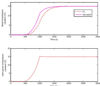
0 500 1000 1500 2000 2500 3000 0 5 10 15 Time (s) M e ta l te m p e ra tu re v a ria ti o n ( °C ) 0 500 1000 1500 2000 2500 3000 0 5 10 15 20 Time (s) In le t ja c k e t te m p e ra tu re v a ri a tio n ( °C ) CL Set point
Fig. 9. Metal body temperature at the outlet position and the inlet jacket temperature after a ramp disturbance onqg0.
Fig. 9 shows the evolution of the metal temperature at the outlet axial position and the corresponding set point T mJ as calculated by the optimization layer. The disturbance causes a progressive change in the set-point, so that the conversion remains as close as possible to the desired conversion despite the presence of the disturbance onqg0. Fig. 9 also highlights the fact that the inner loop controller ensures the metal temperature remains at the set point T mJ thereby allowing the system to reject the disturbance on the inlet gas flow rate.
0 500 1000 1500 2000 2500 3000 0.95*Tfo Tfo Time (s) In le t F lu id T e m p e ra tu re ( K ) 0 500 1000 1500 2000 2500 3000 97 97.5 98 98.5 99 99.5 100 Time (s) C o n v e rs io n ( % )
Fig. 10. Closed loop conversion behavior after a ramp disturbance onTf0.
Let us now analyze the closed-loop behavior of the mini-reactor after a ramp disturbance to the inlet bulk fluid temperature. Fig. 10 shows the conversion’s evolution which demonstrates the performance of the control law which fully compensates for this disturbance. 0 500 1000 1500 2000 2500 3000 0 5 10 15 20 25 30 Time (s) M e ta l te m p e ra tu re v a ri a ti o n (° C ) 0 500 1000 1500 2000 2500 3000 0 5 10 15 20 Time (s) In le t ja c k e t te m p e ra tu re v a ri a ti o n (° C ) CL Set point
Fig. 11. Metal body temperature at the outlet position and the inlet jacket temperature after a ramp disturbance on Tf0. Fig. 11 shows set point evolution T mJ as calculated by the optimization layer and the metal body temperature as assumed at the outlet position of the mini-reactor. The metal body temperature follows the set point with a satisfactory evolution that guarantees an industrially applicable evolution of the manipulated variableTj0.
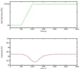
As far as a ramp disturbance on the bulk fluid flow rate is concerned, Fig. 12 shows that the proposed control law fully compensates for this disturbance.
0 500 1000 1500 2000 2500 3000 qlo 1.05*qlo Time (s) In le t F lu id F lo w ( m 3/s ) 0 500 1000 1500 2000 2500 3000 97 97.5 98 98.5 99 99.5 100 Time (s) C o n v e rs io n ( % )
Fig. 12. Closed loop conversion behavior after a ramp disturbance on ql0.
Fig. 13 shows that the behavior of J m
T and 0 j
T is also applicable. The entropy-based controller has shown to perform well in
this case too.
0 500 1000 1500 2000 2500 3000 0 5 10 15 20 Time (s) M e ta l te m p e ra tu re v a ri a ti o n ( °C ) 0 500 1000 1500 2000 2500 3000 0 5 10 15 20 Time (s) In le t ja c k e t te m p e ra tu re v a ri a ti o n ( °C ) CL Set point
Fig. 13. Metal body temperature at the outlet position and inlet jacket temperature behaviors after a ramp disturbance onql0. Let us now consider in more detail the behavior of the inner loop output feedback. To this end, we should examine how the availability function J
m
A is calculated. For each new sample period, the optimizer layer calculates a new set point J mk
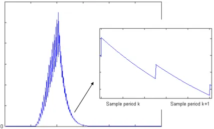
T for the inner loop control layer. Thus, a new availability functionAJ (t)
mk , is defined with respect to TmkJ as represented on Fig. 15: a
new tangent line is defined with respect to the new steady-state set point. Consequently, a sudden increase in AJ (t)
mk occurs, followed by a smooth decrease due to the inner control loop action. This
) ( ) ( 1 1 k mk k mk t U t U + + ) (k+1 mk t A ) ( 1 k mk t A +
S
m U 1 + mk U mk UFig. 14. Availability function evolution at sample time.
Fig. 15. Time evolution ofAmJ in the event of a ramp disturbance on ql0.
The availability function decreases during a sample period k and rises sharply to a new initial value at the beginning of the next sample period k+1. As is can be seen in Figure 15, the availability function finally converges to zero when the system reaches the steady state. Except at the instantstk, the time derivatives of J
m
A remain strictly negative and the availability function plays the role of a Lyapunov function.
As previously mentioned, the reactor body, due to its size, plays the role of an energy absorber that is favorable to reactor stabilization. In order to illustrate this point, we have simulated the behavior of the closed loop reactor with a smaller body
mass by keeping the same controller tuning, with the case of a disturbance on ql0 used as an example. Figure 16 shows the
evolution of the metal temperature at the outlet axial position, the corresponding set point T mJ as calculated by the optimization layer, and the manipulated variableT . This figure highlights the fact that a decrease in the reactor’s body mass greatly affects j0 the evolution of the manipulated variable 0
j
T as well as that of the state variables that exhibit oscillatory behavior. This
simulation confirms the influence of the size of the reactor body on the system’s behavior.
0 500 1000 1500 2000 2500 3000 -5 0 5 10 15 20 25 Time (s) M e ta l te m p e ra tu re ( °C ) CL Set point 0 500 1000 1500 2000 2500 3000 0 5 10 15 20 25 30 Time (s) In le t ja c k e t te m p e ra tu re v a ri a ti o n ( °C )
Fig.16. Metal body temperature at the outlet position and inlet jacket temperature behavior after a ramp disturbance on ql0in
the case of lower reactor mass.
In conclusion, we can notice that the disturbances considered here are satisfactorily rejected by the controller (qg0, f0
T andql0) with a satisfactory evolution of the manipulated variableTj0. Indeed, and as mentioned in Section 2, only these disturbances greatly affect the behavior of the reactor. Both reactant A and B are pure components at the reactor inlet, so their flow rates as well as their temperature are easily measurable. Note that the proposed control law does not deal with modeling error. The reactor is sensitive to certain parameters such as the inlet gas-liquid mass transfer 0
gl glAa
k mass and the heat transfer
coefficient hj [52].
In the presence of modeling errors or unknown disturbances, the performance of the control system will generally degrade,and the stability is guaranteed only in the case of bounded input uncertainties. Thus, the use of a state estimator to reconstruct unmeasured variables would be necessary to lead to better performance of the control system. In this work, the mass and heat transfer coefficients were obtained from experimental results. However, further investigation will be undertaken into the rejection of non-measured disturbances and robustness of the approach with respect to plant-model mismatch.
Conclusions and future works
Intensified continuous mini-reactors working in high pressure and temperature conditions and with very efficient stirring systems, such as the RAPTOR® designed by the French company AETGROUP SAS, are particularly effective at coping with mass transfer limitations during three-phase catalytic reactions. In this paper, we describe a control law based on irreversible thermodynamics. This approach has been found to be well-suited to this type of reactor due to specific energetic features related to a high (reactor body mass)/(bulk mass) ratio.
The situation under consideration is that of a jacketed continuous intensified chemical mini-reactor used to perform three-phase o-cresol catalytic hydrogenation. A dynamic model of this system is proposed. The control objectives are to maintain a high steady-state outlet conversion of the reactant and to operate safely, despite the presence of measured disturbances on the inlet bulk fluid flow rate, the inlet gas flow rate or the inlet fluid flow temperature. In line with industrial practice, the manipulated variable is the inlet jacket temperature. The validity of this choice is confirmed by a steady-state sensitivity study. The control of the process is obtained by using a two-layer approach. The upper layer of the control structure is an optimization layer, using a sequential quadratic programming algorithm that calculates the set point for the lowest layer. The lowest control layer is based on the concavity of the entropy function and the use of the thermodynamic availability as a Lyapunov function. The proposed control scheme is simple and based on measurements easily available in an industrial context. Simulated scenarios show an industrially applicable evolution of the inlet jacket temperature to reject disturbances. Nonetheless, further investigations will be undertaken to look at the rejection of non-measured disturbances and robustness of the approach with respect to plant-model mismatch. Moreover, it would be very interesting to compare this approach based on the thermodynamics of irreversible systems with other control techniques such as Model Predictive Control. Finally, the case of the batch or fed-batch reactors that are extensively used in the fine chemicals industry will also be addressed in future works since in this case, there is no steady state. In this case, a reference trajectory to be tracked has to be determined by dynamic optimization.
Acknowledgments
This project on the intensification of fine chemicals workshops has been supported by the French research agency, the ANR (Agence Nationale de la Recherche).
NOTATION
a interfacial area, m-1
CA concentration of the component A, mol. m-3
* A
C solubility of the component A, mol. m-3
CB concentration of the component B, mol. m-3
Cp heat capacity, J K-1.kg-1
F molar flow, mol. s-1
He Henry’s constant, Pa.m3.mol-1
h heat transfer coefficient, W. m-2.K-1
J molar flux, mol. m-2. s-1
k kinetic constant, mol. kg-1 s-1
K adsorption constant, m3.mol-1
kl mass transfer coefficient gas–liquid, m. s-1
ks mass transfer coefficient liquid–solid, m. s-1
Nb hydrogen bubble number
P pressure, Pa q volume flow, m3. s-1
R reaction rate, mol. kg-1. s-1
rb hydrogen bubble radius, m
S entropy, J. K-1. mol-1
S surface, m2
ST surface of reactor section, m2
T temperature, K
V volume, m3
U internal energy, J
GREEK LETTERS
∆rH heat of reaction, J. mol-1 µ chemical potential, J. mol-1
ν stoichiometric coefficient
α back mixing coefficient
ρ density, kg. m-3 εg gas hold up εl bulk hold up εs solid hold up SUBSCRIPT A component A B component B j jacket fluid f fluid g gas k reactor number l liquid m metal
o reference steady state
s solid SUPERSCRIPT J number of reactors k reactor number I inlet O outlet
References
[1] F. Stoessel, What is your thermal risk?, Chemical Engineering Progress. (1993) 68-75.
[2] S. Lomel, L. Falk, J. M. Commenge, J. L. Houzelot, K. Ramdani, The microreactor. A systematic and efficient tool for the transition from batch to continuous process, Chemical Engineering Research and Design. 84 (A5) (2006) 363-369.
[3] J. C. Charpentier, In the frame of globalization and sustainability, process intensification, a path to the future of chemical and process engineering (molecule into money), Chemical Engineering Journal. 134 (2007) 84-92.
[4] J. C. Etchells, Process intensification. Safety Pros and Cons, Process Safety and Environmental Protection. 83(B2) (2005) 85-89.
[5] R. Aris, N. Amundson, An analysis of chemical reactor stability and control, Chemical Engineering Science. 7(8) (1958) 121–131.
[6] M. Morari, E. Zafiriou, Robust Process Control, Englewood Clims, NJ: Prentice-Hall (1989).
[7] A. Uppal, W. H. Ray, A. B. Poore, On the dynamic behaviour of continuous stirred tank reactors, Chemical Engineering Science. 29 (1976) 967–985.
[8] L. C. Limqueco, J. C. Kantor, Nonlinear output feedback control of an exothermic reactor, Computers and Chemical Engineering 14 (1990) 427–437.
[9] C. Kravaris, C. B. Chung, Nonlinear state feedback synthesis by global input/output linearization, AIChE Journal. 33 (1987) 592–599.
[10]D. Dochain, Design of adaptive linearizing controllers for non-isothermal reactors, International Journal of Control. 59 (1994) 689–710.
[11]J. Alvarez-Ramirez, A. Morales. PI control of continuously stirred tank reactors: stability and performance, Chemical Engineering Science. 55 (2000) 5497-5507.
[12]J. Alvarez-Ramirez, Stability of a class of uncertain continuous stirred chemical reactors with a nonlinear feedback, Chemical Engineering Science. 49 (1994) 1743–1748.
[13]J. Alvarez-Ramirez, R. Suarez, R. Femat, Control of continuous-stirred tank reactors: Stabilization with unknown reaction rates, Chemical Engineering Science. 51(17) (1996) 4183–4188.
[14]H. Ramírez, D. Sbarbaro, R. Ortega. On the control of non-linear processes: An IDA–PBC approach, Journal of Process Control, 19 (2009) 405-414.
[15]R. Antonellia, A. Astolfi, Continuous stirred tank reactors: easy to stabilise?, Automatica. 39 (2003) 1817-1827.
[16]C. Chen, C. Dai, Robust controller design for a class of nonlinear uncertain chemical process, Journal of Process Control. 11 (2001) 469-482.
[17]C. Chen, S. Peng, Design of a sliding mode control system for chemical processes, Journal of Process Control. 15 (2005) 515–530.
[18]R. B. Warden, R. Aris, N. R. Amundson, An analysis of chemical reactor stability and control-VIII. The direct method of Lyapunov. Introduction and applications to simple reactions in stirred vessels, Chemical Engineering Science. 19 (1964) 149-172.
[19]W. R. Dammers, M. Tels, Thermodynamic stability and entropy production in adiabatic stirred flow reactors, Chemical Engineering Science. 29 (1974) 83-90.
[20]C. Georgakis, On the use of extensive variables in process dynamics and control, Chemical Engineering Science. 41 (1986) 1471-1484.
[21]A. Favache, D. Dochain, Thermodynamics and chemical systems stability: The CSTR case study revisited, Journal of Process Control. 19 (2009) 371–379.
[22]A. A. Alonso, B. E. Ydstie, Process systems, passivity and the second law of thermodynamics, Computers and Chemical Engineering. 20(2) (1996) 1119-1124.
[23]B. E. Ydstie, A. A. Alonso, Process systems and passivity via the Clausius-Planck inequality, Systems Control Letters. 30(5) (1997) 253-264.
[24]A. A. Alonso, B. E. Ydstie, Stabilization of distributed systems using irreversible thermodynamics, Automatica. 37 (2001) 1739-1755.
[25]M. Ruszkowski, V. Garcia-Osorio, B. E. Ydstie, Passivity based control of transport reaction systems, AIChE Journal. (2005) 51(12) 3147-3166.
[26]E. C. V. De Toledo, P. L. De Santana, M. R. Wolf Maciel, R. M. Filho, Dynamic modelling of a three-phase catalytic slurry reactor, Chemical Engineering Science. 56 (2001) 6055–6061.
[27]M. C. Rezende, A. C. Costa and M. Filho, Control and optimization of a Three Phase Industrial Hydrogenation Reactor, International Journal of Chemical Engineering. 2 (2004) A21.
[28]D. N. C. Melo, E. C. V. De Toledo, M. M. Santos, S. D.M. Hasan, M. R. Wolf Maciel, M. Regina, R. M. Filho, Off-line optimization and control for real time integration of a three-phase hydrogenation catalytic reactor, Computers and Chemical Engineering. 29 (2005) 2485–2493.
[29]M. C. A. F. Rezende , R. Maciel Filho, A. C. Costa, R. A. Rezende, Algorithms for real-time integrated optimization and control: one layer approach, International Symposium on Advanced Control of Chemical Processes. (2006).
[30]D. N.C. Melo, C. B. Borba Costa, E. C. V. De Toledo, M. M. Santos , M. R. Wolf Maciel, and R. M. Filho, Evaluation of control algorithms for three-phase hydrogenation catalytic reactor, Chemical Engineering Journal. 141 (2008) 250–263. [31]H. Hoang, F. Couenne, C. Jallut, Y. Le Gorrec, Thermodynamic approach for Lyapunov based control, International
Symposium on Advanced Control of Chemical Processes, ADCHEM ’09, Istanbul, Turkey (2009) 367-372.
[32]H. Hoang, F. Couenne, C. Jallut, Y. Le Gorrec, Lyapunov based control for non isothermal continuous stirred tank reactor, in: Proceedings of the 17th World Congress of the IFAC, July 6-11, 2008, Seoul, Korea.
[33]W. Benaissa, N. Gabas, M. Cabassud, D. Carson, S. Elgue, M. Demissy, Dynamic behaviour of a continuous heat exchanger/reactor after flow failure, Journal of Loss Prevention in the Process Industries. 21 (2008) 528-536.
[34]I. Bergault, M. V. Rajashekharam, R. V. Chaudhari, D. Schweich, H. Delmas, Modeling and comparison of acetophenone hydrogenation in trickle-bed and slurry airlift reactors, Chemical Engineering Science. 52 (1997) 4033–4043.
[35]C. Julcour, F. Stüber, J. M. Le Lann, A. M. Wilhelm and H. Delmas, Dynamics of a three-phase up-flow fixed-bed catalytic reactor, Chemical Engineering Science. 54 (1999) 2391–2400.
[36]A. Pinto Mariano, E. C. V. De Toledo, J. M. F. Da Silva, M. R. Wolf Maciel, R. M. Filho, Computers and Chemical Engineering. 29 (2005) 1369–1378.
[37]P. A. Ramachandran, J. M. Smith, Dynamics of three phase slurry reactor, Chemical Engineering Science. 32 (1977) 873– 880.
[38]P. L. Santana, E. C. V. De Toledo, L. A. C. Meleiro, R. Scheffer, N. B. Freitas Jr., M. R. Wolf Maciel, R. M. Filho, A Hybrid mathematical model for a three-phase industrial hydrogenation reactor, European symposium on computer aided process engineering. 11 (2001) 279–284.
[39]J. Wärnä, T. Salmi, Dynamic modelling of catalytic three phase reactors, Computers in Chemical Engineering. 20(1) (1996) 39–47.
[41]S. Choulak, F. Couenne, Y. Le Gorrec, C. Jallut, P. Cassagnau, A. Michel, A generic dynamic model for simulation and control of reactive extrusion, IEC Res. 43(23) (2004) 7373-7382.
[42]S. Bahroun, C. Jallut, C. Valentin, F. De Panthou, Dynamic modelling of a three-phase catalytic slurry intensified chemical reactor, Proceedings of the IFAC ADCHEM 2009, International Symposium on Advanced Control of Chemical Processes, Istanbul, Turkey, July 12-15 (2009) 862-867.
[43]H. Hichri, A. Armand, J. Andrieu, Kinetics and slurry-type reactor modelling during catalytic hydrogenation of o-cresol on Ni/SiO2, Chemical Engineering Process. 30 (1991) 133–140.
[44]D. Kondepudi, I. Prigogine, Modern thermodynamics. From heat engines to dissipative structure, Wiley and Sons (1998). [45]H. B. Callen, Thermodynamics and an introduction to thermostatistics, 2nd edition, Wiley and Sons (1985).
[46]P. Glansdorff P, I. Prigogine, Thermodynamic theory of structure, stability and fluctuations, Wiley-Interscience (1971). [47]S. I. Sandler, Chemical and Engineering Thermodynamics, 3rdedition, Wiley and Sons (1999).
[48]J.P. Corriou, Commande des procédés, second ed., Lavoisier, Tec & Doc, Paris, 2003.
[49]D.E. Seborg, T.F. Edgar, D.A. Mellichamp, Process Dynamics and Control, second ed., John Wiley, 2004. [50]M. Van de Wal, B. de Jager, A review of methods for input/output selection, Automatica. 37 (2001) 487-510.
[51]S. Skogestad, Planwide control : the search for the self-optimizing control structure, Journal of Process Control. 10 (2000) 487-507.
[52]Svandová Z, Markos J, Jelemenský L., Impact of Mass Transfer Coefficient Correlations on Prediction of Reactive Distillation Column Behaviour, Chemical Engineering Journal. 140 (2008) 381-390.
[53]S. R. de Groot and P. Mazur, Non-equilibrium thermodynamics, first ed., Dover Publications Inc., Amsterdam, 1962, pp. 457.
[54]J.Vidal, Thermodynamics Applications in chemical Engineering and the Petroleum Industry, Editions TECHNIP, Paris, 2003, pp.145.
[55]H. Hoang, « Approche thermodynamique pour la stabilisation des réacteurs chimiques » in French. Ph.D thesis, Université de Claude Bernard Lyon 1, France (2009).