This is an author-deposited version published in : http://oatao.univ-toulouse.fr/ Eprints ID : 8802
To link to this article : DOI: 10.1007/s11242-012-0040-y URL : http://dx.doi.org/10.1007/s11242-012-0040-y
O
pen
A
rchive
T
OULOUSE
A
rchive
O
uverte (
OATAO
)
OATAO is an open access repository that collects the work of Toulouse researchers and makes it freely available over the web where possible.
To cite this version :
Davit, Yohan and Wood, Brian D. and Debenest, Gérald and Quintard, Michel Correspondence Between One- and
Two-Equation Models for Solute Transport in Two-Region Heterogeneous Porous Media. (2012) Transport in Porous Media, vol. 95 (n° 1). pp. 213-238. ISSN 0169-3913
Any correspondence concerning this service should be sent to the repository administrator: staff-oatao@listes.diff.inp-toulouse.fr
Correspondence Between One- and Two-Equation
Models for Solute Transport in Two-Region
Heterogeneous Porous Media
Y. Davit · B. D. Wood · G. Debenest · M. Quintard
Abstract In this work, we study the transient behavior of homogenized models for solute transport in two-region porous media. We focus on the following three models: (1) a time non-local, two-equation model (2eq-nlt). This model does not rely on time constraints and, therefore, is particularly useful in the short-time regime, when the timescale of interest (t) is smaller than the characteristic time (τ1) for the relaxation of the effective macroscale
param-eters (i.e., when t ≤ τ1); (2) a time local, two-equation model (2eq). This model can be
adopted when (t) is significantly larger than (τ1) (i.e., when t ≫ τ1); and (3) a one-equation,
time-asymptotic formulation (1eq∞). This model can be adopted when (t) is significantly larger than the timescale (τ2) associated with exchange processes between the two regions
(i.e., when t ≫ τ2). In order to obtain insight into this transient behavior, we combine a
theoretical approach based on the analysis of spatial moments with numerical and analytical results in several simple cases. The main result of this paper is to show that there is only a weak asymptotic convergence of the solution of (2eq) towards the solution of (1eq∞) in terms of standardized moments but, interestingly, not in terms of centered moments. The physical interpretation of this result is that deviations from the Fickian situation persist in the limit of long times but that the spreading of the solute is eventually dominating these higher order effects.
Y. Davit (
B
)University of Oxford, Mathematical Institute, 24–29 St. Giles’, Oxford, OX1 3LB, UK e-mail: davit@maths.ox.ac.uk
B. D. Wood
School of Chemical, Biological and Environmental Engineering, Oregon State University, Corvallis, OR 97331, USA
G. Debenest· M. Quintard
Université de Toulouse; INPT, UPS; IMFT (Institut de Mécanique des Fluides de Toulouse), Allée Camille Soula, 31400 Toulouse, France
G. Debenest· M. Quintard
Keywords Porous media· Homogenization · Volume averaging · Dispersion · Spatial moments
List of Symbols Variables
bi j Closure mapping vector in the i -region associated with∇hcjij (m)
ci Pointwise solute concentration in the i -region (mol m−3) hcii Superficial spatial average of ci(mol m−3)
hciii Intrinsic spatial average of ci(mol m−3)
hciγ ω Weighted spatial average concentration (mol m−3)
˜ci Solute concentration standard deviation in the i -region (mol m−3)
Di Diffusion tensor in the i -region (m2s−1)
Di j Dispersion tensor in the two-equation models associated with ∂thciii and 1hcjij (m2s−1)
Di j Dispersion coefficient in the 1-D two-equation models associated with ∂thciii and 1hcjij (m2s−1)
D∞ Dispersion tensor of the one-equation time-asymptotic model (m2s−1)
D∞ Dispersion coefficient of the 1-D one-equation time-asymptotic model (m2s−1) exp Exponentially decaying terms (−)
h Transient effective mass exchange kernel (s−1)
h∞ Effective mass exchange coefficient (s−1)
˜ji Deviation of the total mass flux for region i (mol m−2s−1)
Ji Average of the total mass flux for region i (mol m−2s−1)
L Characteristic length of the field-scale (m) ℓi Characteristic length of the i -region (m)
min nth-order centered moment associated with hciii for the two-equation model (mnmol)
mγ ωn nth-order centered moment associated with hciγ ω for the two-equation model (mnmol)
m∞n nth-order centered moment associated with hciγ ω for the one-equation asymptotic model (mnmol)
Mnγ ω nth-order standardized moment associated with hciγ ω for the two-equation model (−)
Mn∞ nth-order standardized moment associated withhciγ ωfor the one-equation asymp-totic model (−)
ni j Normal unit vector pointing from the i -region towards the j -region (−)
pk Three lattice vectors that are needed to describe the 3-D spatial periodicity (m)
Qi(x,t ) Macroscopic source term in the i -region (mol m−3s−1)
Qγ ω Weighted macroscopic source term (mol m−3s−1)
R Radius of the REV, (m)
Si j Boundary between the i -region and the j -region (−)
Si j Area associated withSi j (m2)
ri Closure parameter in the i -region associated withhcγiγ − hcωiω (−)
t Time (s)
t’ Non-dimensionalized time (−)
T Period of the oscillations (s)
hvii Superficial spatial average of vi (m s−1) hviii Intrinsic spatial average of vi (m s−1)
hviii Norm of the intrinsic spatial average of vi (m s−1) ˜vi Velocity standard deviation in the i -region (m s−1)
Vi j Effective velocity in the two-equation models associated with ∂thciii and ∇hcjij (m s−1)
V∞ Effective velocity of the one-equation time-asymptotic model (m s−1)
Vi Domain of the averaging volume that is identified with the i -region (−)
Vi Volume of the domainVi (m3)
V Domain of the averaging volume (−)
V Volume of the domainV (m3)
Greeks
α Weighted mass transfer coefficient, h∞ ! 1 Φγεγ + 1 Φωεω " (s−1) β∗1and β∗2 Source terms in the closure problems (m s−1)
γ-region First region (−)
1V Velocity contrast between the γ and ω regions, Vγ γ − Vωω(m s−1)
1D Dispersion contrast between the γ and ω regions,Dγ γ − Dωω (m2s−1)
Φi i − region volume fraction (−)
εi Darcy-scale fluid fraction (porosity) within the i -region (−) ω-region Second region (−)
τ1 Characteristic time for the relaxation of the two-equation model effective
param-eters (s)
τ2 Characteristic time for the transition towards the one-equation asymptotic
regime (s)
µin nth-order raw moment associated with the hciii for the two-equation model (mnmol)
µγ ωn nth-order raw moment associated with the hciγ ω for the two-equation model (mnmol)
µ∞n nth-order raw moment associated with the hciγ ω for the one-equation asymp-totic model (mn mol)
Subscript
i, j Indices for γ or ω (−)
1 Introduction
The physics of transport in porous media deals inevitably with multiscale heterogeneities (Cushman 1997). A number of theoretical and numerical methods have been developed to model these systems. The most direct approach is to solve the transport equations at the sub-pore scale by directly computing solutions with sufficient resolution over an enormous number of pores. Contemporary computational methods have begun to make this approach possible. However, such detailed microscale solutions generally contain a substantial amount of information that is of low value to most applications. To provide results with practical rel-evance, tensor fields at the microscale can generally be filtered by eliminating the small-scale
Fig. 1 Schematic diagram highlighting the hierarchy of the main scales involved in solute transport in
two-region porous media. The macroscale is characterized by the length L; the support scale, associated with V, is characterized by the radius R; and the microscale (Darcy-scale) regions are characterized by lengths ℓγ and ℓω. Throughout this paper, homogenization of microscale equations relies on the following inequalities:
L ≫ R ≫ ℓγ, ℓω
high frequency fluctuations. Various upscaling techniques have been developed for this pur-pose, where one first averages the partial differential balance equations that apply at the microscale, and then solves these averaged equations at a coarser scale of resolution. This kind of approach always requires the solution of ancillary closure relations to provide repre-sentations of how the small-scale correlations influence the solution at the macroscale. Such techniques have been widely used to model transport problems in porous media and example approaches include volume averaging (Whitaker 1999), ensemble averaging (Dagan 1989;
Cushman and Ginn 1993), moments matching (Brenner 1980), and multiscale asymptotics (Bensoussan et al. 1978). An overview of upscaling methods has recently been provided by
Cushman et al.(2002).
In this article, we are interested in comparing the behavior of several different upscaled models for describing solute transport via convection and diffusion in a discretely hierarchical porous medium containing two different regions consisting of coarse and fine porous media (see Fig.1). In this figure, we have illustrated three characteristic scales in the sequence of scales in the hierarchy: (1) the macroscale associated with the volume VM and the charac-teristic length L; (2) the support scale associated with the volume of the averaging operator,
V, and the characteristic length R; and (3) the microscale associated with the size of a
repre-sentative volume of porous material within the coarse and fine regions and the characteristic lengths ℓγ and ℓω.
Under the most general conditions, the transport process applying at the macroscale is specified by a differential balance equation that is time and space non-local; such transport equations have been widely reported in the literature, and have been developed from a number of different upscaling approaches (e.g.,Koch and Brady 1987;Cushman and Hu 1995;Wood 2009). This behavior can be mathematically described via solutions of integro-differential equations that involve convolutions of a memory kernel over space and time. These non-local macroscale formulations are extremely important from a theoretical point of view and have also been applied to the description of transport phenomena in heterogeneous porous media (Cushman et al. 1995). However, there are also a number of computational and physical issues that lower their practical value. For example, with most discrete numerical methods, spatial convolutions lead to dense matrices that are much more complicated to invert than the sparse matrices produced by purely local models (Wood 2009). Without additional approx-imations regarding the evolution of the kernels, non-local models may not actually reduce the information content as compared with the direct solution to the microscale problem.
To make these equations more tractable, various simplifications to the exact non-local models have been considered (e.g.,Chastanet and Wood 2008;Haggerty et al. 2004). These simplifications often rely on conjectures about the time and space scales of the transport processes with the general goal of localizing equations, i.e., transforming integro-differen-tial formulations into systems of parintegro-differen-tial differenintegro-differen-tial equations. The local models that result from this procedure have more restricted domains of validity but are generally simpler to solve; the difficulty being to determine the best compromise for a specific application. In this paper, we will consider three approximations to the exact non-local description in the case of two-region porous media: (1) a two-equation, non-local in time model (2eq-nlt); (2) a time and space local two-equation model (2eq); and (3) an asymptotic in time one-equation model (1eq∞). Each of these models is briefly described below.
The time non-local two-equation model examined here corresponds to the developments byMoyne(1997);Souadnia et al.(2002) andWood and Valdès-Parada(2012). The model is specified by
Model 1: Two-equation, time non-local(2eq-nlt)
∂thcγiγ + # j=γ,ω ∂tVγj · ⋆∇hcjij = # j=γ,ω ∇ · ! ∂tDγj · ⋆∇hcjij " − ∂th Φγεγ ⋆$hcγiγ − hcωiω% + Qγ, (1) ∂thcωiω+ # j=γ,ω ∂tVωj · ⋆∇hcjij = # j=γ,ω ∇ ·!∂tDωj · ⋆∇hcjij " − ∂th Φωεω ⋆$hcωiω− hcγiγ% + Qω. (2)
In these equations,hciii refers to the intrinsic volume averaged concentration in the i -region. The bracket notationh·i is here as a reminder that the concentrations appearing in this two-equation model are defined as volume averages of the pointwise concentrations ciat the micro-scale. The ⋆ operator refers to convolutions in time defined by e ⋆ f (t)=&0te (τ ) f (t−τ )dτ .
The product A· ⋆B is the mixed contraction (·) /time convolution (⋆) between tensor fields
A and B. The macroscale parameter Φi is the volume fraction of the i -region, considered constant in time and space; εi is the Darcy-scale volume fraction of fluid phase within the
i-region, considered constant in time and space; the macroscale parameters, Vi j andDi j, are intrinsic velocities and dispersion tensors of the two-equation model (Vi jandDi j with i 6= j are interphase coupling terms for the macroscale fluxes); the parameter h is a macroscale mass exchange kernel; and Qiis a source term. In terms of the volume averaging theory, this formulation refers to situations in which the concentration perturbations are well captured by the two-equation spatial localization process; but which require a fully transient closure. Effective parameters, Vi j,Di j, and h, are defined as integrals of mapping variables that solve initial boundary value problems (IBVPs) at the microscale. Hence, in Eqs. (1) and (2), the convolution kernels are generic functions and can be related to a specific porous medium via computation of these IBVPs over a representative volume. In practice, if the topology of the microscale problem is unknown, the kernels may be approximated by heuristic functions (seeHaggerty et al. 2000;Luo et al. 2008). We also remark that this local in space/non-local in time approach is adapted to situations for which the non-locality in time is weakly cou-pled with the non-locality in space and the temporal convolutions can be treated separately from the spatial convolutions. This is the case, for instance, for a periodic mobile–immobile system for which the time convolution will capture all the relaxation times for diffusion in the immobile domain.
A second set of approximations leads to a formulation that is both local in time and space. The particular model examined here corresponds to the developments ofAhmadi et al.(1998) andCherblanc(2003,2007):
Model 2: Local two-equation(2eq)
∂thcγiγ + # j=γ,ω Vγj · ∇hcjij = # j=γ,ω ∇ ·!Dγj · ∇hcjij " − h∞ Φγεγ $hc γiγ − hcωiω% + Qγ, (3) ∂thcωiω+ # j=γ,ω Vωj · ∇hcjij = # j=γ,ω ∇ · ! Dωj · ∇hcjij " − h∞ Φωεω $hcωi ω − hcγiγ% + Qω. (4)
This model is valid when the characteristic times for the relaxation of the effective parameters are very small compared to the macroscopic time of interest. In this case, the convolutions disappear, i.e., we have ∂tA (t)· ⋆B (t) ≈ A (∞) · B (t), (cf. Sect. 4.1 and 4.2 inChastanet
and Wood (2008) andDavit and Quintard (2012)). The relaxation of the convolution ker-nels and the convergence of ∂tA (t)· ⋆B (t) towards A (∞) · B (t) are both controlled by the characteristic times of the IBVPs discussed above. An attractive feature of this model is the unique coefficient, h∞, whereby mass exchange processes between the two regions are described. In this way, spatial heterogeneities may be accounted for by simply considering a spatial distribution of h∞, seeKfoury et al. (2004,2006). The disadvantage of this model when compared with the (2eq-nlt) model is that it will fail to describe transport processes in the short-time regime when the convolutions must be considered (Parker and Valocchi 1986;Landereau et al. 2001). Other possible descriptions are multirate mass transfer models (Haggerty and Gorelick 1995), but we will limit our study to the fully non-local and fully local two-equation descriptions, Eqs. (1)–(2) and (3)–(4).
The third, and last, set of approximations that we will consider leads to the one-equation time-asymptotic formulation, as described byQuintard et al.(2001):
Model 3: Time-asymptotic, one-equation(1eq∞)
∂thciγ ω+ V∞· ∇hciγ ω = ∇ ·$D∞∇hciγ ω% + Qγ ω. (5) In Eq. (5),hciγ ωis the weighted average solute concentration over the regions (γ ) and (ω):
hciγ ω ≡ Φγεγhcγi
γ
+ Φωεωhcωiω
Φγεγ + Φωεω
. (6)
V∞ is the solute weighted average velocity,
V∞ ≡ Φγεγhvγi γ
+ Φωεωhvωiω
Φγεγ + Φωεω
, (7)
where hviii is the volume average velocity over the phase (i );D∞ is the time-asymptotic dispersion tensor (seeDavit et al. 2010for a detailed expression); and Qγ ω is the weighted average source term. In the literature, this model has been derived using, at least, two differ-ent techniques.Zanotti and Carbonell(1984) studied the asymptotic behavior of the spatial moments of (2eq) in a semi-infinite medium and used the relationshipD∞ ≡ 12tlim→∞
d dt !mγ ω 2 mγ ω0 " , where mγ ωn is the nth-order centered spatial moment associated withhciγ ω, to derive an ana-lytical expression for D∞. A more direct one-step derivation can be obtained by averaging over the two phases simultaneously and using a non-conventional perturbation decomposition (seeDavit et al. 2010).
The purpose of this work is to gain insight into the correspondence between these three different models. More specifically, the contributions of this study are to
1. illustrate the transient behavior of all three models by studying analytical solutions to the purely diffusive problem with periodic excitations in a “space-clamped” stratified geometry.
2. examine the convergence of solutions for the two-equation (2eq) and one-equation (1eq∞) models as time increases. In particular, we are interested in developing a con-straint that indicates when one can use the one-equation time-asymptotic model (1eq∞) given by Eq. (5) instead of the two-equation model (2eq) given by Eqs. (3)–(4). For the expression of this constraint, we consider the propagation of a pulse through an infi-nite one-dimensional porous medium. We will not study the influence of the boundary conditions on the time-asymptotic regime (see discussions inDavarzani 2010).
The remainder of this article is organized as follows. In Sect.2, we briefly outline the deri-vation of the three macroscale models described above using the volume averaging theory. In Sect.3, we illustrate the frequency response of all three models by studying analytical solutions to the purely diffusive transport problem. In Sect.4, we analyze Eqs. (3)–(4) using spatial moments and study their asymptotic behavior. We also compute the corresponding spatial moments up to the sixth order and show that these numerical results support the theoretical analysis.
2 Macroscale Models Derivation
2.1 Preliminaries and Definitions
In this section, we provide a brief presentation of the volume averaging technique and discuss the derivation of the three models described above. The purpose here is to provide only an outline; the details of these derivations can be found in the original papers referenced for each of the three models.
For these developments, we consider two different regions (cf. Fig.1) in which the solute undergoes diffusion and convection: we can think of these two regions as being associated with a binary distribution of coarse and fine porous media. We assume a continuity of the concentrations and of the fluxes at the boundary between the coarse (γ ) and fine (ω) regions. The microscale mass balanced equations take the form
γ-region: ∂t$εγcγ% + ∇ · $εγcγvγ% = ∇ · $εγDγ · ∇cγ%, in Vγ, (8a) BC1: cω = cγ, on Sγ ω, (8b) BC2: −nγ ω· εγDγ · ∇cγ = −nγ ω· εωDω· ∇cω, on Sγ ω, (8c) ω-region: ∂t(εωcω)+ ∇ · (εωcωvω)= ∇ · (εωDω· ∇cω), in Vω, (8d) IC1: cγ = 0, in Vγ at t < 0, (8e) IC2: cω = 0, inVω at t < 0. (8f)
In these equations, ci (i = γ, ω) is the concentration in the i-region and we impose uni-formly zero initial concentrations. In addition, the velocity field, vi, is assumed to be known pointwise for the purposes of this study. This is correct if the flow problem, i.e., the total mass and momentum balance equations can be solved independently, which is the case if the component is a tracer. The reader may refer toQuintard and Whitaker(1998) for a derivation of regional Darcy’s laws which may be used in conjunction with the equations derived in this paper.Dγ is the Darcy-scale dispersion tensor.Si j is the interface between the i - and the
j-region, and Si jis the area of this interface; ni jis the corresponding normal unit vector point-ing from i to j . We remark that these equations are based on the assumption that a continuum description holds for representative volumes defined at a length scale that is smaller than ℓγ
and ℓω, i.e., Eqs. (8a)–(8f) already represent an average Darcy-scale description where the
averaging has been used to homogenize the pore-scale details. An important consequence of this heterogeneous configuration is the appearance of the Darcy-scale porosities εi(i = γ, ω); porosities that we will consider constant in time and space throughout this work.
To obtain a macroscopic model for mass transport, we average each microscopic equa-tion over a representative region (REV) and use the following quantities:Vi represents the
i-region within the REV and Vi is the volume of Vi. The superficial averages of ci over the volume V are given by hcii ≡ V1
&
Vi ci dV . The associated intrinsic averages for ci
are hciii ≡ V1 i
&
Vi ci dV . We define the constant volume fractions as Φi ≡
Vi
V ; with this definition implying thathcii = Φihciii.
2.2 Perturbation Analysis
During the averaging process, terms involving point values of cγ, cω, vγ, and vω appear in
the integrands. To treat these terms, one conventionally defines perturbation decompositions for any property ϕi(where i indicates the region, so that i is either γ or ω) by ϕi = hϕiii+ ˜ϕi. Upon imposing the separation of length scales, ℓγ, ℓω ≪ R ≪ L, it is possible to show that
the volume averaged equations take the form (see Appendix A):
∂t ! Φiεihciii " + ∇ · ! Φiεihciiihviii " = ∇ · ΦiεiDi · ∇ hcii i + 1 Vi -Sγ ω ni j˜cidS +1 V -Sγ ω ni j · εiDi · ∇ ˜cidS− ∇ · ! Φiεih ˜ci˜viii " . (9)
Equation (9) represents a macroscopic description of the transport processes. However, because unknown deviation quantities appear in the equation, the problem is not in a closed form. In order to close the problem, we need to: (1) determine the IBVPs that the perturbations satisfy; and (2) use the solutions of these IBVPs to obtain a closed form of Eq. (9).
The definition of the perturbations, ˜ci ≡ ci − hciii, suggests that the set of equations governing ˜ci can be obtained by subtracting suitable multiples of Eq. (9) from Eqs. (8a) and (8d). This operation leads to a problem of the form
∂t˜ci + ∇ · ( ˜civi)− h∇ · ( ˜civi)ii + ˜vi · ∇hciii = ∇ · (Di · ∇ ˜ci)− h∇ · (Di∇ ˜ci)ii, (10a) BC1: ˜cγ − ˜cω = −$hcγiγ − hcωiω%, on Sγ ω, (10b) BC2: nγ ω· ! ˜jγ − ˜jω " = −nγ ω ·$Jγ − Jω%, on Sγ ω, (10c) where ˜ji ≡ −εiDi· ∇ ˜ci, Ji ≡ −εiDi· ∇hciii, andh∇ · (Di∇ ˜ci)ii = V1i & Sγ ω ni· Di· ∇ ˜cidS. To ensure uniqueness of ˜ci, we impose the zero initial condition ˜ci(t = 0) = 0, the solvability conditionh ˜ciii = 0 and local periodicity.
At this point, Eq. (10) are still coupled with the macroscopic concentrations but in a weaker sense. One can look for a solution of the form (see Moyne et al.; Souadnia et al. 2002;Valdes-Parada and Alvarez- Ramirez 2011;Davit and Quintard 2012):
˜ci = #
j=γ,ω
∂tbi j · ⋆∇hcjij − ∂tri ⋆$hcγiγ − hcωiω%, (11)
where the microscale fields, b and r , may be interpreted as spatial integrals of the corre-sponding Green’s functions (see discussions inWood 2009;Wood and Valdès-Parada 2012). This mathematical structure for the fluctuations is conditioned by the source terms in Eq. (10) and, therefore, by the localization approximations, ℓγ, ℓω ≪ R ≪ L, that have been made
previously.
On substituting Eq. (11) into Eq. (10), we can obtain a unit cell IBVP that can be used to calculate the microscale fields, b and r (see Appendix B).
2.3 Macroscopic Models
We can now use Eq. (11) into Eq. (9) to eliminate unknown deviation concentrations from macroscale equations. The result of this operation leads to Eqs. (1) and (2); seeMoyne et al.; Souadnia et al. 2002for more details. Transient effective parameters are expressed as integrals of the microscale fields, b and r , which are given in Appendix C.
To understand the correspondence between Eqs. (1)–(2) and (3)–(4), it is useful to con-sider the transient behavior of the integrands and the relaxation of the convolution ker-nels. For example, h (t) undergoes a transient regime and then reaches a stationary state, i.e., after a given relaxation time τ1 (say, the smallest eigenvalue of the unit cell IBVP),
h (t ) tends towards a constant exchange rate h∞ (more exactly, within the convolution,
h (t ) may be approximated by u(t)h∞ where u(t) is the unit step function). Therefore, ∂th ⋆$hcγiγ − hcωiω% ≈ h∞δ (t ) ⋆$hcγiγ − hcωiω% = h∞$hcγiγ − hcωiω%, where δ (t) is
the Dirac distribution. The relaxation time, τ1, is determined by the IBVP in the unit cell and
a similar approximation can be made for other effective kernels (see discussion in Moyne 1997;Souadnia et al. 2002).
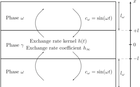
Fig. 2 Schematic diagram illustrating the stratified space-clamped configuration with sinusoidal excitation.
The concentration field within the phase (ω) is uniform (space clamped) and sinusoidal, cω = sin (ωt). For simplicity, we will also consider the case Φγ = 1.0 which corresponds to the limit lω → 0, i.e., the phase (ω)can be treated as a boundary condition
To derive the one-equation time-asymptotic model, Eq. (5), two techniques have been pre-viously used.Zanotti and Carbonell(1984) used an asymptotic analysis of the first two cen-tered spatial moments of (2eq) in a semi-infinite medium. A more direct one-step derivation can be obtained by averaging over the two phases simultaneously and using a non-conven-tional perturbation decomposition (seeDavit et al. 2010). However, both approaches do not provide clear limitations for the validity of this approximation. In the approach devised by
Zanotti and Carbonell (1984), higher order spatial moments have been neglected and it is unclear how this may affect solutions. With the other approach, constraints are expressed in terms of scaling constraints of the concentration perturbations; constraints which are not necessarily straightforward to interpret in real applications.
To gain insight into the nature of these constraints, we develop in Sect.3analytical solu-tions in a simple case and illustrate the transient behavior of the models. In Sect.4, we use the framework proposed inZanotti and Carbonell(1984) to study higher order moments in a one-dimensional situation.
3 Convergence of Solutions of the (2eq-nlt), (2eq) and (1eq∞
) Models: An Example for the Case of Pure Diffusion
In this section, our goal is to gain insight into the long-time behavior of the three different models presented above. In the general case, solutions to these equations require numerical computations. To simplify our study, we will focus on analytical solutions in the case of pure diffusion in a “space-clamped” stratified medium (see detailed description in Fig.2). Stratified geometries have been used extensively as model systems (cf., literature cited throughout this paper) because they capture the physics of the problem while allowing dimen-sional reduction. Furthermore, we will focus on the relatively simple case of a sinusoidal excitation, so that the macroscopic signal is fully characterized by the period of the oscil-lations, T ≡ 2πω . We remark that this problem is not necessarily of particular importance to applications but it does allow to gain insight into the long-time behavior of the models.
Without loss of generality, we also fix εγ = Φγ = 1.0 so that we can treat the phase ω as a
boundary condition (lω → 0 in Fig.2).
3.1 Models
The microscale diffusion problem boils down to the one-dimensional parabolic equation, ∂tcmicroγ = Dγ
∂2cmicroγ
∂x2 , (12)
with−l < x < +l, zero initial concentration, and the boundary conditions x = ±l main-tained at sin (ωt) for t ≥ 0. With regard to the macroscopic models, Eq. (1) takes the form:
dhcγ⋆iγ dt + d dth ⋆hc ⋆ γiγ = d dth ⋆sin (ωt). (13)
Equation (3) may be written as: dhcγiγ
dt +h∞hcγi
γ
= h∞sin (ωt), (14)
Equation (5) corresponds to the local mass equilibrium situation, hcγ∞i
γ
= sin (ωt). (15)
In these equations, we have used the superscripts ⋆ and ∞ to denote the non-local and asymptotic models, respectively.
3.2 Analytical Solutions
Since we have imposed a spatially uniform concentration on the boundary, the non-local model is exact and hcγ⋆iγ can be determined via direct integration of the analytical solu-tion to Eq. (12); a solution which can be found in Carslaw and Jaeger (1946). Discarding exponentially decaying terms, this operation yields
hc⋆γiγ t =
→∞Csin(ωt + D), (16)
with C = 4
(hA sin (χ)iγ)2+ (hA cos (χ)iγ)2, D = arctan!hA sin(χ)iγ
hA cos(χ)iγ " , χ = arg 5 cosh kx(1+i) cosh kl(1+i) 6 ,A = 4 cosh 2kx+cos 2kx
cosh 2kl+cos 2kl and k =
4 ω
2Dγ . For the solution of the local two-equation model, we apply Laplace transforms to Eq. (14) and obtain,
hcγiγ = t→∞ h∞ 7 h2 ∞+ ω2 sin 8 ωt − arctan 8 ω h∞ 99 . (17)
For our purposes, we also need to determine a characteristic time (τ1) for the relaxation
of h (t) and the corresponding asymptotic value for the exchange rate, h∞. Equation (63) may be written as h = 2l1 &−l+lDγ∂
rγ
∂x dx with rγ solution of the following partial differential equation,
∂trγ = Dγ
∂2rγ
with the boundary condition rγ = 1 onSγ ω. To facilitate solution, we decompose rγ into
rγ = 1 − Rγ ⋆ ∂∂thwhere Rγ solves
∂tRγ = Dγ
∂2Rγ
∂x2 + 1, (19)
with the boundary condition Rγ = 0 onSγ ω. The solution of Eq. (19) is (seeCarslaw and
Jaeger 1946) Rγ = l2 2Dγ : 1− x 2 l2 − 32 π3 ∞ # n=0 (−1)n (2n+ 1)3 cos (2n+ 1) π x 2l e −Dγ(2n+1)2π2 t/4l2 ; , (20)
and the expression of h is derived from< Rγ
=γ
⋆ ∂th (t )= 1, e.g., by Laplace transform inver-sion procedures. We can now extract the smallest eigenvalue in Eq. (20) to obtain τ1= 4l
2
π2D γ and the stationary part of Eq. (20) yields h∞= 3Dγ
l2 . 3.3 Results
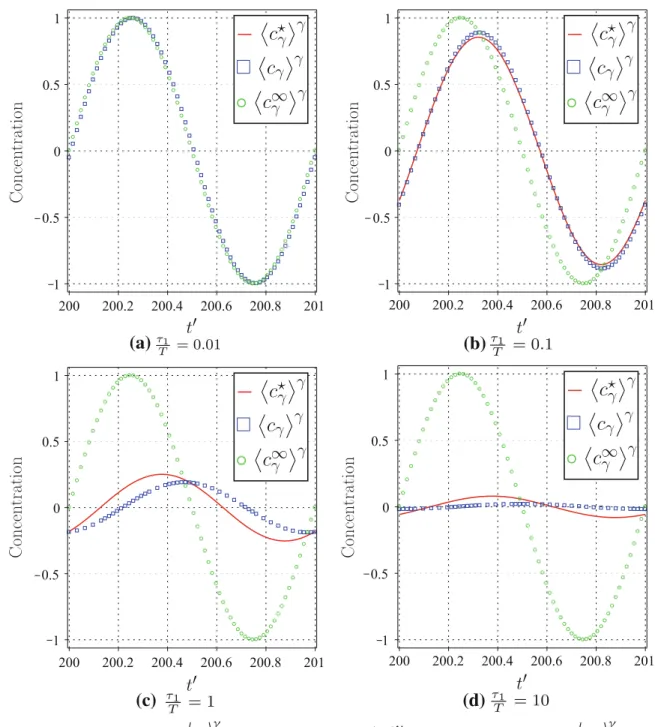
To plot solutions, we fix l = 0.5 and the time t is non-dimensionalized with T = 2πω , i.e., t′ = Tt = 2πω t. Results are presented in Fig.3 for different ratios τ1
T =
2l2 π3D
γ ω, after relaxation of the exponentially decaying terms. Figure 4shows the behavior of the phases and amplitudes of the three models with varying τ1
T. These results illustrate two specific transient behavior. First, it shows that Eq. (15) is only valid in the strict limit τ1
T → 0, when the phases and amplitudes of all three models converge to a unique value. Second, it shows that the solution of Eq. (13) converges towards the solution of Eq. (14) when τ1 ≪ T . More
generally, this suggests that Eqs. (3) and (4) represent a good approximation of Eqs. (1) and (2) under the condition that T ≫ τ1where τ1can be estimated via
τ1 ≡O > sup ? lγ hvγiγ , lω hvωiω , l 2 γ Dγ , l 2 ω Dγ @A , (21) and T via T ≡O ! inf5Thcγiγ,Thc ωiω,T∇hcγiγ,T∇hcωiω,T∇2hcγiγ,T∇2hcωiω 6" . (22)
In these equations, Tϕ is the characteristic time associated with ϕ.
To overcome the short-time limitations of the local two-equation model, one could use an exchange coefficient, h∞, that depends on the frequency of the oscillations, ω, in Eqs. (3) and (4), i.e., without convolutions. For instance, such an approach was proposed in the case of transient dispersion in porous media and is discussed inDavit and Quintard(2012). Equating amplitudes and phases of Eqs. (16) and (17) yields the following values for the exchange rate:
(a) (b)
(c) (d)
Fig. 3 (Color online) Plots ofBcγ⋆Cγ (red line 2eq non-local),<cγ=γ (blue squares 2eq local) and B
c∞γ Cγ (green
circles1eq) as functions of t′ = Tt, for various ratios τ1
T . Here, we have used l= 0.5 and εγ = Φγ = 1.0. These plots were obtained in MAPLE™ by using the analytical solutions given in Eqs. (16), (17) and (15). They show that: (1) Eq. (15) is only valid in the strict limit τ1
T → 0; and (2) (red line 2eq non-local) may be approximated by (blue squares 2eq local) when τ1≪ T
hamplitude(ω)
ω ≡
4
(hA sin (χ)iγ)2+ (hA cos (χ)iγ)2 4
1− (hA sin (χ)iγ)2− (hA cos (χ)iγ)2
, (23) and, hphase (ω) ω ≡ − hA cos (χ)iγ hA sin (χ)iγ . (24)
To illustrate the behavior of these expressions, we have plotted hamplitudeω and hphaseω as func-tions of τ1
T in Fig. 5. Results show that
hamplitude
ω and
hphase
Fig. 4 (Color online) Plots of the amplitude and phase ofBc⋆γCγ (red line 2eq non-local),<cγ=γ (blue squares 2eq local) andBcγ∞Cγ (green circles 1eq) as functions of the ratio τ1
T = ω
2l2
π3Dγ. Here, we have used l= 0.5
and εγ = Φγ = 1.0. These plots were obtained in MAPLE™by using the amplitude and phase of analytical solutions given in Eqs. (16), (17) and (15). Similarly to Fig3, they show that: (1) Eq. (15) is only valid in the strict limit τT1 → 0; and (2) (red line 2eq non-local) may be approximated by (blue squares 2eq local) when τ1≪ T
Fig. 5 (Color online) Plots of hphase/ω (red circles) andhamplitude/ω (blue squares) as functions of τ1
T =
ω 2l2
π3Dγ. These plots were obtained in MAPLE
™by using analytical solutions given in Eqs. (24) and (23). They show that h∞ cannot be adjusted to the frequency of the oscillations becausehphase/ω ≃ hamplitude/ω only in the low-frequency limit when two-equation models are not necessary and the one-equation asymptotic model can be used.
τ1
T → 0, where two-equation models are not needed and the asymptotic formulation can be adopted. This shows that it is not possible to recover the phase and the amplitude of the signal simultaneously and that the exchange rate, h∞, cannot be adjusted to the frequency of the oscillations.
4 Convergence of Solutions of the (2eq) and (1eq∞
) Models: Spatial Moments Analysis
In this Section, we consider the convergence of the solution of the (2eq) model to the solution of (1eq∞) with increasing time. Our analysis will focus primarily on the spatial moments of the two models, with our goal being to show that the properly conditioned moments of the two models converge as time grows.
4.1 Preliminaries and Definitions
Moments are mathematical tools that can be used to analyze the shape of spatial/temporal sig-nals. They have been used for a variety of purposes, including studies of solute breakthrough curves in soils, e.g., inStagnitti et al.(2000); the behavior of fractional advection–diffusion equations (seeZhang 2010); mixing in heterogeneous porous media (seeChiogna et al. 2011); model parameter estimations from column experiments, e.g., inYoung and Ball(2000); and analytical solutions in dual-permeability media inXu and Hu(2004).
Here, our study is based on developments performed by Zanotti and Carbonell (1984) who used spatial moments to study the asymptotic behavior of (2eq) for the propagation of a pulse in an infinite medium. An interesting conclusion from this analysis is that the distance between the spatial signals, hcγiγ and hcωiω, tend towards a constant Ω in the long-time
limit, not towards 0. This result suggests that the macroscopic concentration fields, hcγiγ
andhcωiω, are two separate entities, even in the asymptotic regime and this is unclear how a
single macroscopic concentration,hciγ ω, may be used to describe solute transport. To study this phenomenon, we will use the following spatial moments (see for exampleGovindaraju and Bhabani 2007):
1. Raw spatial moments for intrinsic average concentrations of the (2eq) model:
µin(t )≡
+∞
-−∞
xnhciiidx. (25)
2. Raw spatial moments for the weighted average concentration of the (2eq) model:
µγ ωn (t )≡
+∞
-−∞
xnhciγ ωdx. (26)
3. Centered spatial moments for intrinsic average concentrations of the (2eq) model:
min ≡ +∞ -−∞ ! x − µi1 "n hciiidx. (27)
4. Centered spatial moments for the weighted average concentration of the (2eq) model: mγ ωn ≡ +∞ -−∞ $x − µγ ω1 %n hciγ ωdx. (28)
5. Standardized spatial moments for the weighted average concentration of the (2eq) model:
Mnγ ω ≡
mγ ωn
$mγ ω2 %n2 . (29)
The corresponding spatial moments for the (1eq∞) model will be denoted by the superscript ∞: µ∞n , m∞n , and Mn∞. We will also use the following functional,
δn ≡ D D D D D mγ ωn − m∞n $m∞ 2 %n2 D D D D D , (30)
to measure deviations of the (2eq) model from the (1eq∞) model.
In order to understand how these moments can be used to describe the asymptotic behavior of the two-equation model, we briefly review below their physical interpretation. The raw spatial moments characterize the shape of the signal in a fixed referential. For example, the first-order moment corresponds to the mean position and the second-order moment describes the net spreading. If the mean position is transient, µ1(t ), the second-order moment will
account for the spreading relative to the mean and for the spreading due to the movement of the mean. With dispersion effects, one is only interested in the spreading relative to the mean which is the information captured by the second-order centered moments, m2. More
gener-ally, centered moments, mn, describe the shape of the signal in the referential moving with µ1(t ). We can further rescale centered moments with the second-order moment to obtain
standardized moments that may be used to measure the relative importance of higher order moments compared with the spreading. Following this idea, we can characterize differences between solutions and convergence properties using the definition given in Eq. (30).
4.2 Assumptions
To simplify the analysis, we will use the following assumptions:
1. The domain is treated as an infinite medium in which we assume that there is no mass in the system at t < 0.
2. We consider only the case where the initial condition is specified by a delta inpulse, i.e.,
Qγ(x , t ) = Qω(x , t ) = δ(x)δ(t). The goal of this assumption is only to simplify the
results; more complex initial conditions can be found from such a solution by simple convolutions.
3. We assume that Vγ ω ≪ Vγ γ, Vωγ ≪ Vωω,Dγ ω ≪ Dγ γ, andDωγ ≪ Dωω. Physically,
Vi i andDi i contain the leading order terms; Vi j andDi j are often neglected, e.g., for the mobile–immobile models (seeCoats and Smith 1964).
Note that the goal of hypotheses 2 and 3 is primarily to facilitate the presentation of the theo-retical analysis. Although the results are not presented in this paper, we studied numerically (similarly to what we present in Sect.4.6) the effect of these hypotheses, and did not observe a significant (qualitative) modification of the results for typical 1D problems.
4.3 Spatial Moments Analysis of the Two-Equation Local Model (2eq)
The easiest way to determine the spatial moments of Eqs. (3) and (4) is to compute them directly from analytical solutions to the transport problem. However, there is no analyti-cal solution for the general form of the two-equation model, so an alternative approach is required. A balance equation for the moments themselves can be determined by multiplying Eqs. (3) and (4) by xnand integrating by parts to obtain the following result
dµγn dt = n (n − 1) Dγ γµ γ n−2+ nVγ γµ γ n−1− h∞ Φγεγ $µγn − µωn % for n ≥ 2, (31) dµωn dt = n (n − 1) Dωωµ ω n−2 + nVωωµωn−1− h∞ Φωεω $µω n − µ γ n % for n ≥ 2, (32) with µγ0 = µω0 = 1, µγ ω1 = V∞t and, V∞ ≡ ΦγεγVγ γ + ΦωεωVωω Φγεγ + Φωεω . (33)
This leads to the following expression for the weighted central second-order moment: 1 2m γ ω 2 = − 3 2 ΦγεγΦωεω $Φγεγ + Φωεω %2Ω 2 + D∞t+ exp, (34) with D∞≡ # i, j=γ,ω Φiεi Φγεγ + ΦωεωD i j + ΦγεγΦωεω $Φγεγ + Φωεω %2 1V2 α . (35)
In these equations, we have used 1V = Vγ γ − Vωω, Ω = α11V where Ω represents the
shift/distance between the two signals at long times (see Fig.6 andZanotti and Carbonell 1984), and
α ≡ Φγεγ + Φωεω ΦγεγΦωεω
h∞. (36)
Fig. 6 (Color online) Schematic diagram illustrating the transition from the pre-asymptotic to the asymptotic
regime. The picture shows that the net spreading,√2D∞t, will eventually dominate higher order deviations from normality, δn ≪ 1 ∀n ≥ 2 for t ≫ h1
For simplicity, we have also grouped exponentially decaying terms of the form tme−kαt, where m and k are positive integers, into the unique notation exp. We remark that, on con-sidering the time-infinite limit of Eq. (34), we have reached the same conclusions than in
Zanotti and Carbonell(1984) and have found an equivalent expression forD∞.
For centered moments, an analytical calculation up to the sixth order leads to the following conclusion,∀n ≥ 2: mγ ωn = (n − 1)!!$2D∞t %n2 +O ! tn2−1 "
+ exp for n even, (37)
mγ ωn =O !
tn−12 "
+ exp for n odd, (38)
with (n− 1)!! = E i;0≤2i<n−1
(n− 1 − 2i). A formal derivation of these relationships is rather tedious, so that we briefly outline below a methodology that may be used to prove these results. The first step towards solution is to extract µγn (µωn) from Eq. (31) (Eq. (32) respectively), which yields µωn = µγn + Φγεγ h∞ dµγn dt − Φγεγ h∞ Fn (n − 1) Dγ γµ γ n−2 + nVγ γµ γ n−1G, (39) µγn = µωn + Φωεω h∞ dµωn dt − Φωεω h∞ Fn (n − 1) Dωωµ ω n−2+ nVωωµωn−1G . (40) Then, we may uncouple Eqs. (31) and (32) by substituting Eq. (39) into Eq. (32) and Eq. (40) into Eq. (31). The result of these operations can be expressed as a second-order ordinary differential equation on µγ ωn and then on mγ ωn (i.e., by considering the moving frame with velocity V∞) that may be used to perform a recurrence analysis and demonstrate Eqs. (37)–(38).
For the standardized moments, it is thus straightforward to show that:
Mnγ ω = (n − 1)!! +O 8 1
t
9
+ exp for n even, (41)
Mnγ ω = O 8 1 √ t 9
+ exp for n odd. (42)
4.4 Spatial Moments Analysis of the One-Equation Time-Asymptotic Model (1eq∞) Following a similar technique, the moments of the one-equation model can be determined by multiplying Eq. (5) by xnand integrating by parts to obtain the following relationship:
dµ∞n
dt = n (n − 1) D
∞µ∞
n−2+ nV∞µ∞n−1, n ≥ 2, (43) with µ∞0 = 1 and µ∞1 = V∞t. A similar approach was used byLuo et al.(2008) to determine the temporal moments. To calculate these moments, we could also use the relationship given byAris(1958). From these equations, by considering the frame moving with µγ ω1 , we can determine the centered moments,
m∞n = (n − 1)!!$2D∞t%n2 for n ≥ 2 even, (44)
The standardized moments, defined in Eq. (29), are:
Mn∞ = (n − 1)!! for n ≥ 2 even, (46)
Mn∞ = 0 for n ≥ 2 odd. (47)
In particular, we have the skewness of the Gaussian signal, M3∞ = 0, and the kurtosis,
M4∞ = 3.
4.5 Theoretical Analysis of the Convergence
From Eq. (34), we can obtain the first constraint for the validity of the one-equation approx-imation. We require that t ≫ α1 in order to relax the exponentially decaying terms. Equiv-alently, we will write this constraint as t ≫ h1
∞ by assuming Φγεγ ∼ Φωεω and avoid the simpler case where the volume fraction weighting simplifies the analysis.
Even when these exponential terms are relaxed, we see, from Eqs. (37)–(38) and Eqs. (44)– (45) that centered moments of Eqs. (3)–(4) do not converge towards those of Eq. (5). This is particularly clear when considering the behavior of odd-order centered moments, which are non-zero for the two-equation model, Eq. (38), and zero for the one-equation model, Eq. (45). However, by comparing Eqs. (41)–(42) with Eqs. (46)–(47) and considering the long-time limit, we see that there is a convergence of solutions in terms of standardized moments. In par-ticular, we have limt→∞M3γ ω = M3∞ = 0 for the skewness and limt→∞M4γ ω = M4∞ = 3 for the kurtosis. The physical interpretation of these results is that one never rigorously obtains a normal distribution of the concentrations, but the spreading (the second-order cen-tered moment) is eventually dominating higher order deviations from the Fickian situation (higher order moments). This phenomenon is illustrated in Fig.6.
To develop clear constraints that apply to any order, we define a metric, δn, that mea-sures the normality of the signal. In conjunction with the constraint for the relaxation of the exponential terms, t ≫ h1
∞, we require that, for n ≥ 2:
δn = D D D D D mγ ωn − m∞n $m∞ 2 %n2 D D D D D ≪ 1, (48)
This constraint, for the second order, yields 3 2 ΦγεγΦωεω $Φγεγ + Φωεω %2 Ω2 D∞ ≪ t. (49)
This inequality may be interpreted as the constraint√2D∞t ≫ Ω where√2D∞t is the
net spreading and Ω is the distance between the two signals (see the graphical representation of this constraint in Fig.6). In addition, the definition ofD∞, Eq. (35), supplies
D∞ ≥ ΦγεγΦωεω α$Φγεγ + Φωεω
%21V
2
, (50)
which can be combined with Ω = α11V and Eq. (49) to obtain the following (order of magnitude) sufficient condition for δ2 ≪ 1:
t ≫ 1
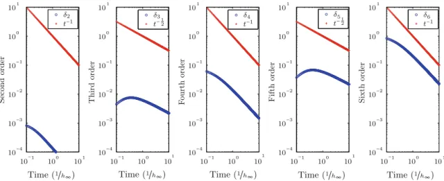
Fig. 7 (Color online) Log–log plots of δn for Φγεγ = 0.7, Φωεω = 0.1, Vωγ = Vγ ω = Dωγ = Dγ ω= 0,
Vγ γ = 2, Vωω = 1, Dγ γ = 10, Dωω = 5 and h∞ = 1. These plots were obtained by computing numeri-cally (MATLABTM, ode15s) Eqs. (31) and (32) to determine the corresponding values of δn up to the sixth order. Results show that there are two different timescales for the evolution of the moments. For small times,
t ≪1/h∞, the dominant terms are the exponential parts. For longer times, t ≫1/h∞, δn tends towards zero as O ! 1 √ t " or O ! 1 t "
This shows that the constraints associated with δ2and exp are the same; although δ2
cor-responds to a weak convergence of the form δ2 =O
$1
t%. An identical analysis can be carried out for higher order moments. It may be summarized as follows:
1. For n = 2k (k ∈ Z+∗), there is correspondence between leading order terms, O$tk%,
of mγ ω2k and m∞2k. Therefore, we have mγ ω2k − m∞2k = O$tk−1% and m∞
2 = O(t )which yields δ2k =O ! tk−1 tk " =O$1 t%.
2. For n = 2k + 1 (k ∈Z+∗), m∞2k+1 = 0 and mγ ω2k+1 = O$tk%, so that mγ ω
2k+1− m∞2k+1 = O$tk%. This yields δ2k+1 =O 8 tk tk+12 9 =O ! 1 √ t " .
At any order, an analysis similar to that of the second order supplies the constraint t ≫ h1 ∞; with a convergence inO$1
t% for even-order moments and inO !
1 √
t "
for odd-order moments. Higher order analytical calculations are extremely tedious so that we will focus, in Sect.4.6, on a numerical confirmation of the behavior of δn up to the sixth order.
4.6 Numerical Analysis of the Convergence
Equations (31) and (32) were computed numerically to determine the values of δn up to the sixth order. We used MATLAB™ environment with the ode15s solver to compute these solutions; a relative tolerance of≈ 2x10⁻¹⁴was adopted for the solver. The moments com-puted are presented in Fig. 7 for δn, up to sixth order, with Φγεγ = 0.7, Φωεω = 0.1,
Vωγ = Vγ ω = Dωγ = Dγ ω = 0, Vγ γ = 2, Vωω = 1, Dγ γ = 10, Dωω = 5 and h∞ = 1.
The results are presented in a log–log graph; examination of the plots shows that there are two different timescales for the evolution of the moments. For small times, t ≪ 1/h∞,
the dominant term is the exponential part. For longer times, t ≫ 1/h
∞, δn monotonically decreases to zero asO ! 1 √ t " andO$1
t%; therefore, corroborating the theoretical results pre-sented above.
5 Discussion and Conclusions
Upscaling techniques aim at filtering information from the microscale to obtain homoge-nized descriptions of the transport phenomena. This filtering process usually takes the form of constraints regarding the space and timescales of the transport processes. However, there is no uniqueness of these constraints and the scaling must be adapted to the physical con-figuration of interest. In this paper, we provided some insight into the transient behavior of models that are specific to the description of solute transport in two-region porous media. We focused on three deterministic formulations that have been previously developed, namely: the two-equation time non-local model, the two-equation time local model and the one-equation time-asymptotic model. Roughly speaking, we may think of these three models as approx-imations of the exact non-local formalism; approxapprox-imations that are particularly well suited to the two-region problem: the two-equation time non-local model may be seen as second order in space, non-local in time; the two-equation time local model as second order in space and time; and the asymptotic model as first order in space and time.
In the first part of this study, we used the volume averaging theory to derive these three models and discuss the assumptions that are made during upscaling. In the second part of this study, we compared results obtained using the three different models via analytical solu-tions to the purely diffusive transport problem. We focused on a “space-clamped” stratified geometry with periodic Dirichlet boundary conditions. The timescale constraints associ-ated with each formulation were discussed by comparing the period of the oscillations with characteristic times of the partial differential equations. Finally, we studied the asymptotic behavior of the spatial moments of Eqs, (3) and (4) for the propagation of a pulse through an infinite/semi-infinite medium.
The primary result of this paper is to show that there is convergence of the solution of Eqs. (3)–(4) towards the solution of Eq. (5) in terms of standardized moments, but not in terms of centered moments. The physical interpretation of this result is that, in the
asymp-totic regime, higher order deviations from the Fickian situation are increasing at a slower rate than the net spreading; but these deviations are not converging towards zero. This result sheds light on the physics underlying the correspondence between these two models and shows that convergence only occurs in a weak sense. It may also be useful to interpret more general aspects of mass transport in heterogeneous porous media, such as the difference between spreading and mixing. For example,Le Borgne et al.(2010) show that net spreading may scale in a Fickian manner while mixing can persist to scale in a non-Fickian manner. This phenomenon is reminiscent of the idea that, in the asymptotic regime, deviations from the Fickian situation do not disappear, i.e., solutions do not converge in terms of centered moments; but become small compared with the net spreading, i.e., solutions do converge in terms of standardized moments.
Secondary results of this paper can be summarized as follows:
1. We have detailed the derivation of the above three models using the volume averaging and moments matching techniques. We have discussed the domains of validity of the models, as illustrated in Fig.8.
2. We have defined a generic measure of higher order deviations from the asymptotic regime, δn = D D D D mγ ωn −m∞n (m∞2 )n2 D D D
D ∀n ≥ 2, that may be used in a more general manner to compare the behavior of a variety of different models.
3. We have shown in Sect.3 that h∞ cannot be made frequency-dependent and transient effective kernels must be used with convolutions.
Fig. 8 (Color online) Schematic representation of the domains of validity of the different models for a pulse
in a dual-region infinite porous medium. This diagram illustrates three different domains: (1) for t ≪ τ1, non-local formulations are required; (2) for t ≫ τ1, the two-equation local model can be used; and (3) for
t ≫ τ2, the one-equation time-asymptotic model can be used
In essence, this study extends the work ofZanotti and Carbonell(1984) andMoyne(1997);
Moyne et al.;Souadnia et al.(2002);Quintard et al.(2001) in that we solve the issue of higher order moments that was not addressed inZanotti and Carbonell(1984) and study the conver-gence of the solutions of the two-equation and one-equation formulations. When compared with more generic discussions of non-local transport theories with randomly varying fields (seeKoch and Brady 1987,1988;Neuman 1993), the originality of this work is to explore in more details the relationships between three localization procedures and models which are
specific to the two-region problem. Future work will focus on:
– developing a broader comparison of these models with other descriptions, e.g., multirate mass transfer.
– studying the influence of initial/boundary conditions upon these results.
Acknowledgments Support from CNRS/GdR 2990 is gratefully acknowledged. The second author (BDW) was supported in part by the Office of Science (BER), U.S. Department of Energy, Grant No. DE-FG02-07ER64417. This publication was based on work supported in part by Award No KUK-C1-013-04, made by King Abdullah University of Science and Technology (KAUST).
Appendix A
To develop equations governing mass transport at the macroscopic scale, we need to average each Darcy-scale equation:
i-region: h∂t(εici)i + h∇ · (εivici)i = h∇ · (εiDi · ∇ci)i. (52) To interchange derivatives and integrals, we use (1) the general transport theorem for sta-tic interfaces (see Whitaker 1981 or Leibniz rule) and (2) the spatial averaging theorems (seeHowes and Whitaker 1985;Gray et al. 1993). These yield
i-region: ∂t ! Φiεihciii " + ∇ · ! Φiεihciiihviii " = ∇ · ΦiεiDi · ∇ hcii i + 1 Vi -Sγ ω nicidS + 1 V -Sγ ω ni · εiDi · ∇cidS− ∇ · ! Φiεih ˜civiii " . (53)
Further, we use the following decompositions ci = hciii + ˜ci and hciiix+y = hciiix + y · ∇hciiix +O$∇∇hciiix% where x is the vector pointing towards the position of the center of the REV and y is the vector pointing inside the REV. We also neglect terms involving y by imposing R ≪ L (Whitaker 1999), where L is a characteristic field-scale length. This supplies 1 V -Sγ ω nicidS ≃ hciiix 1 V -Sγ ω nidS + 1 V -Sγ ω ni˜cidS. (54)
Using spatial averaging theorems for unity yields V1 &S
γ ωnidS = −∇Φi and since we have assumed constant volume fractions, we can eliminate the first term in the right-hand side of Eq. (54). A similar approximation applied to averaged fluxes and advective terms leads to Eq. (9).
Appendix B
Upon substituting Eq. (11) into Eq. (10), we can collect separately terms involving∇hcγiγ,
∇hcωiω andhcγiγ − hcωiω. For all these problems, we consider only zero initial conditions
and local periodicity.
Collecting terms involvinghcγiγ − hcωiωyields
∂tri + vi · ∇ri = ∇ · (Di · ∇ri)± Φi−1εi−1h (t ), (55a)
BC1: rγ − rω = 1, on Sγ ω, (55b)
BC2: nγ ω·$εγDγ · ∇rγ − εωDω · ∇rω% = 0, on Sγ ω, (55c)
Periodicity: ri(x+ pk)= ri(x), k = 1, 2, 3. (55d)
Using previous assumptions, we can write h (t)≡ Φγεγh∇ ·$Dγ∇rγ%iγ = −Φωεωh∇ ·
(Dω∇rω)iω. The symbol± corresponds to the signs − in the region γ , + in the region ω. We
have used pk to represent the three lattice vectors that are needed to describe the 3-D spatial periodicity. We also have the solvability condition,hriii = 0.
Collecting terms involving∇hcγiγ yields
∂tbi γ + vi ·$∇bi γ − riI% + δi γ˜vi = ∇ ·FDi ·$∇bi γ − riI%G − h˜viriii ± Φi−1ε−1i β∗1, (56a) BC1: bγ γ − bωγ = 0, on Sγ ω, (56b) BC2: nγ ω·F−εγDγ ·$∇bγ γ − rγI% + εωDω ·$∇bωγ − rωI%G = nγ ω· εγDγ,on Sγ ω, (56c) Periodicity: bi j(x+ pk)= bi j(x), k = 1, 2, 3. (56d) Here β∗1 ≡ Φγεγh∇ ·FDγ ·$∇bγ γ − rγI%Giγ = −Φωεωh∇ ·FDω·$∇bωγ − rωI%Giω and
δi j ≡ 1 if i = j, δi j ≡ 0 if i 6= j.The symbol ± corresponds to the signs − in the region γ , + in the region ω. We also have the solvability condition, hbi γiγ = 0.
Collecting terms involving∇hcωiωyields
BC1: bγ ω− bωω = 0, on Sγ ω, (57b)
BC2: nγ ω·F−εγDγ ·$∇bγ ω+ rγI% + εωDω· (∇bωω + rωI)G = −nγ ω· εωDω,on Sγ ω,
(57c) Periodicity: bi j(x+ pk)= bi j(x), k = 1, 2, 3. (57d) where we have used β∗2 ≡ Φγεγh∇ ·FDγ ·$∇bγ ω+ rγI%Giγ = −Φωεωh∇ ·FDω·$∇bωω+
rωI%Giω. The symbol ± corresponds to the signs − in the region γ , + in the region ω. We
also have the solvability condition,hbi ωiω = 0.
Appendix C
Effective velocities, containing intrinsic averages of the microscale velocities, are given by
Vγ γ ≡ hvγiγ − Φγ−1εγ−1β∗1− h˜vγrγiγ, (58) Vωω ≡ hvωiω+ Φω−1εω−1β∗2+ h˜vωrωiω. (59)
Inter-region velocities are given by
Vγ ω ≡ −Φω−1εω−1β∗2+ h˜vγrγiγ, (60) Vωγ ≡ Φγ−1εγ−1β∗1− h˜vωrωiω. (61)
Dispersion tensors are given by
Di j ≡ Di · I + 1 Vi -Sγ ω nibi jdS − h ˜vibi ji i, (62)
and the first-order exchange coefficient reads
h ≡ 1 V -Sγ ω nγ ω· εγDγ · ∇rγdS = − 1 V -Sγ ω nωγ · εωDω· ∇rωdS. (63)
With these definitions, effective parameters exhibit a time-dependence, even though we have used the notationsDi j, Vi j, and h instead ofDi j(t ), Vi j(t ), and h (t).
References
Ahmadi, A., Quintard, M., Whitaker, S.: Transport in chemically and mechanically heterogeneous porous media, V, Two-equation model for solute transport with adsorption. Adv. Water Resour. 22, 59–86 (1998) Aris, R.: Dispersion of linear kinematic waves. Proc. Roy. Soc. Ser. A 245, 268–277 (1958)
Bensoussan, A., Lions, J., Papanicolau, G.: Asymptotic Analysis for Periodic Structures. North-Holland Publishing Company, Amsterdam (1978)
Brenner, H.: Dispersion resulting from flow through spatially periodic porous media. Proc. Roy. Soc. Lond. Ser. A 297(1430), 81–133 (1980)
Carslaw, H., Jaeger, J.: Conduction of Heat in Solids. Clarendon Press, Oxford (1946)
Chastanet, J., Wood, B.: The mass transfer process in a two-region medium. Water Resour. Res. 44, W05413 (2008)
Cherblanc, F., Ahmadi, A., Quintard, M.: Two-medium description of dispersion in heterogeneous porous media: Calculation of macroscopic properties. Water Resour. Res. 39(6), SBH6–1 (2003)