Cortical thickness or grey matter volume? The importance of selecting the phenotype for imaging genetics studies.

(1)

Cortical Thickness or Grey Matter Volume? The Importance of

Selecting the Phenotype for Imaging Genetics Studies

Anderson M. Winklera,b, Peter Kochunovc, John Blangerod, Laura Almasyd, Karl Zillese,f,

Peter T. Foxc, Ravindranath Duggiralad, and David C. Glahna,b,c

Anderson M. Winkler: anderson.winkler@yale.edu

a_{Department of Psychiatry, Yale University School of Medicine, New Haven, CT, USA}

b_{Olin Neuropsychiatry Research Center, The Institute of Living, Hartford, CT, USA}

c_{Research Imaging Center, University of Texas Health Science Center San Antonio, San}

Antonio, TX, USA

d_{Department of Genetics, Southwest Foundation for Biomedical Research, San Antonio, TX,}

USA

e_{Institute of Neuroscience and Medicine (IMN-2), Research Center Jülich, Jülich, Germany}

f_{C. & O. Vogt-Institut fur Hirnforschung, Heinrich Heine Universität, Düsseldorf, Germany}

Abstract

Choosing the appropriate neuroimaging phenotype is critical to successfully identify genes that influence brain structure or function. While neuroimaging methods provide numerous potential phenotypes, their role for imaging genetics studies are unclear. Here we examine the relationship between brain volume, grey matter volume, cortical thickness and surface area, from a genetic standpoint. Four hundred and eighty-six individuals from randomly ascertained extended pedigrees with high-quality T1-weighted neuroanatomic MRI images participated in the study. Surface-based and voxel-based representations of brain structure were derived, using automated methods, and these measurements were analysed using a variance-components method to identify the heritability of these traits and their genetic correlations. All neuroanatomic traits were

significantly influenced by genetic factors. Cortical thickness and surface area measurements were found to be genetically and phenotypically independent. While both thickness and area influenced volume measurements of cortical grey matter, volume was more closely related to surface area than cortical thickness. This trend was observed for both the volume-based and surface-based techniques. The results suggest that surface area and cortical thickness measurements should be considered separately and preferred over gray matter volumes for imaging genetic studies.

Keywords

brain cortical thickness; brain surface area; heritability

Correspondence to: Anderson M. Winkler, anderson.winkler@yale.edu.

URL: http://www.glahngroup.org (David C. Glahn)

Publisher's Disclaimer: This is a PDF file of an unedited manuscript that has been accepted for publication. As a service to our

customers we are providing this early version of the manuscript. The manuscript will undergo copyediting, typesetting, and review of

NIH Public Access

Author Manuscript

Neuroimage. Author manuscript; available in PMC 2011 November 15.

Published in final edited form as:

Neuroimage. 2010 November 15; 53(3): 1135–1146. doi:10.1016/j.neuroimage.2009.12.028.

NIH-PA Author Manuscript

(2)

1. Introduction

Despite evidence that most neurological and psychiatric illnesses are genetically mediated, the identification of genes that predispose brain-related disorders has been difficult. One strategy for unraveling the genetic determinants of these complex illnesses is the use of endophenotypes, also called intermediate phenotypes (Gottesman and Shields, 1967; Gottesman and Gould, 2003), which are quantitative traits that are genetically correlated with illness. Neuroimaging methods provide an array of potential endophenotypes for these disorders (Glahn et al., 2007). Although there is mounting evidence that quantitative indices derived from brain structure and function are heritable (Baaré et al., 2001; Thompson et al., 2001; Geschwind et al., 2002; Peper et al., 2007; Glahn et al., 2007), and associated with neuropsychiatric disorders (McDonald et al., 2006; Honea et al., 2008; Goldman et al., 2008, 2009; van der Schot et al., 2009), it is unclear which genes influence these traits or the biological mechanisms that govern these measurements. The search for genes that influence brain-related traits could be improved by choosing imaging phenotypes that are closest to a single gene action (Wojczynski and Tiwari, 2008). However, given the complexity and multi-dimensional nature of imaging data, it is critical to determine the appropriate measurements to be employed. In this report, we examine issues surrounding the use of imaging-derived grey matter measurements in imaging genetics studies.

Although the human brain is gyrencephalic, with no absolute linear relationship between brain volume and surface area (Hofman, 1985; Armstrong et al., 1995), simple geometric laws still hold within the cortical mantle, where the grey matter volume is defined as the amount of grey matter that lies between the grey-white interface and the pia mater (Figure 1, left). Previous findings suggest that cortical surface area and cortical thickness are

independent, both globally and regionally, that grey matter volume is a function of these two indices and each of these three measurements are heritable (Winkler et al., 2009; Panizzon et al., 2009). Furthermore, Panizzon et al. (2009) reported that surface area and cortical thickness are genetically uncorrelated. Thus, volume measurements, which combine aspects of both traits, are likely influenced by some combination of these genetic factors. Since different definitions of a phenotype potentially lead to different genetic findings (Rao, 2008), it would seem that surface or thickness measures would have advantages over volume measures for gene discovery.

Cortical anatomy, which is structured as a corrugated two-dimensional sheet of tissue, can be well represented by surface models, which facilitate the analysis of relationships between cortical regions and provide superior visualisation (van Essen et al., 1998). Intersubject and even interspecies registration can be accomplished using surface-based representations (van Essen et al., 2001), allowing matching of homologies without relying directly on spatial smoothing as in volume-based methods (Ashburner and Friston, 2000). Computational advances in surface reconstruction (Mangin et al., 1995; Dale et al., 1999; Fischl et al., 1999a) and the availability of software packages also facilitates its use. Despite these advantages, quantitative methods based on purely volumetric representations of the brain are still common. Amongst these, voxel-based morphometry (VBM) (Wright et al., 1995; Bullmore et al., 1999; Ashburner and Friston, 2000; Good et al., 2001) is a relatively fast, straightforward method, that quantifies the amount of grey matter existing in a voxel and permits a comparison across subjects (Figure 1, right). VBM requires that voxels are classied according to different tissue types, usually grey matter, white matter and

cerebrospinal fluid (GM/WM/CSF). To allow comparison across subjects, images are non-linearly aligned to standard brain, where a common coordinate system can be defined, and volumes are corrected for local shrinkages and expansions using the Jacobian determinants of the warps at each voxel (Good et al., 2001). In this way, VBM allows for the

NIH-PA Author Manuscript

(3)

quantification of the grey matter volumes, globally and regionally, using either the voxels directly or regions of interest.

In this study, we compare measurements obtained with VBM methods, with measurements from surface-based representations of the brain in genetically informative samples. We focus our attention to determining the genetic control over (1) the volume of the grey matter computed using surface-based and volume-based representations of the brain, (2) the cortical surface area and (3) the cortical thickness.

2. Method

2.1. Participants

Subjects participated in the Genetics of Brain Structure and Function Study, GOBS, a collaborative effort involving the Southwest Foundation for Biomedical Research, the University of Texas Health Science Center at San Antonio (UTHSCSA) and the Yale University School of Medicine. To date, more than 1000 individuals from randomly selected families of Mexican-American ascent, who live in San Antonio, Texas, USA, have been

recruited. The data presented here is based on the analysis of the T1-weighted MRI images

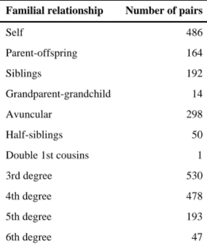
from the 486 subjects scanned before December 31st, 2008. A summary of the pedigree structure is presented on Table 1. The mean age of this group was 48.6±13.2 years (min = 26.1, max = 85.1) and 302 were females. All participants provided written informed consent on forms approved by the institutional review board at the UTHSCSA.

2.2. Acquisition of Images

The images were acquired at the Research Imaging Center, UTHSCSA, using a Siemens

MAGNETOM Trio 3 T system (Siemens, Erlangen, Germany), with a high-resolution, T1

-weighted, 3D Turbo-FLASH sequence with an adiabatic inversion contrast pulse with the following scan parameters: TR/TI/TE = 2100/785/3.04 ms, flip angle = 13°, voxel size (isotropic) = 0.8 mm. Each subject was scanned 7 (seven) times, consecutively, using the same protocol, and a single image was obtained by linearly coregistering these images and computing the average, allowing improvement over the signal-to-noise ratio and reducing motion artifacts (Kochunov et al., 2006).

2.3. Processing of Images

Image analysis followed two separate pathways: the generation of surface representations of the cortex and the segmentation of the brain into GM, WM and CSF, in their voxel-based representation. The first part was conducted using the FreeSurfer software package (Athinoula A. Martinos Center for Biomedical Imaging, Harvard University, Cambridge, MA, USA), while the second was performed using the FMRIB Software Library – FSL (Oxford Centre for Functional MRI of the Brain, University of Oxford, UK).

2.3.1. Surface-based Analysis—The surface-based analysis followed the procedures

described by Dale et al. (1999) and Fischl et al. (1999a). Images are corrected for magnetic field inhomogeneities, affine-registered to the Talairach-Tournoux atlas (Talairach and Tournoux, 1988) and skull-stripped. The voxels belonging to the WM are identified based on their locations, on their intensities and on the intensities of the neighbouring voxels. The two hemispheres are separated and the WM voxels are grouped into a mass of connected voxels using a six-neighbours connectivity scheme. A mesh of triangular faces is tightly built around the WM, using two triangles per exposed voxel face. The mesh is smoothed using an algorithm that takes into account the local intensity in the original images (Dale and Sereno, 1993), at a subvoxel resolution, using trilinear interpolation. Topological defects are corrected (Fischl et al., 2001) ensuring that the surface has the same topological properties

NIH-PA Author Manuscript

(4)

of a sphere. A second iteration of smoothing is applied, resulting in a realistic representation of the interface between grey and white matter. This surface is referred to simply as white

surface. The external cortical surface, which corresponds to the pia mater, is produced by

nudging outwards the white surface towards a point where the tissue contrast is maximal, maintaining constraints on its smoothness and on the possibility of self-intersection (Fischl and Dale, 2000). This surface is referred to simply as the pial surface.

These surfaces are parcellated into smaller regions using an automated process (Fischl et al., 2004). For each subject, this is done by first homeomorphically mapping the pial surface to a spherical coordinate system (Fischl et al., 1999b), where the folding patterns are matched to an average map. An a priori atlas of probabilities for regions of interest is used in a

Bayesian approach to establish probabilities that a given vertex belongs to a certain label. In a second, iterative step, the surface is treated as an anisotropic, non-stationary Markov random field, where for each vertex, the labels assigned to its neighbours are also

considered. The labelling is iterated until no vertices change their assignments (Fischl et al., 2002, 2004). We used the regions of the atlas developed by Desikan et al. (2006), recently modified to include the insula as an independent region of interest (Figure 2).

2.3.2. Volume-based Analysis—The volume-based pipeline started with skull-stripped

images produced in an intermediate step of the surface-based pipeline, allowing a direct comparison between the methods. Images were segmented in GM, WM and CSF using the FAST module of FSL, which models the problem of classification into different classes as a hidden Markov random field (HMRF), an extension of hidden Markov models that assumes that the observations come from an underlying Markov random field (Kunsch et al., 1995). Thus, the assignment of a voxel to a class depends on its immediate spatial neighbours in the three-dimensional space, and the problem is treated by obtaining the maximum likelihood estimate of the parameters using an expectation-maximization (EM) algorithm (Zhang et al., 2001). The output of this HMRF-EM framework is an image where the value at each voxel corresponds to the proportion of the volume of the voxel that is occupied by a tissue class. Estimation of these partial volume effects for each voxel is of paramount importance here, as it allows one to compute the amount of a certain class of tissue present in a region by summing the partial volume effects at each voxel of that region. The segmentation as described above operated in the images in the subject space, not transformed to a standard coordinate space. The subsequent analyses were conducted in the subject space as well, obviating the need to correct the intensities of voxels for local stretchings or shrinkages.

2.3.3. Combining Surface-based and Volume-based Analyses—Voxels identified

inside the space delimited by the pial and white surfaces were classified as belonging to the cortex, producing a representation of the cortical mantle in terms of voxels, tractable in a VBM-like approach. The cortex was further parcellated in the same scheme as the surface representation by assigning to each cortical voxel the same label as the closest vertex in the surfaces.

For each region defined in the voxel-based representation, the volume of grey matter was computed by integrating the partial volume effects from the images segmented using the HMRF-EM algorithm. From the surface-based representations, regional measurements for average cortical thickness, surface area and grey matter volume were obtained. Area was measured at the white suface. Global measurements for area and the grey matter volume were computed by summing the values of the parcellations, whereas a global measure of the average thickness was obtained by weighting the regional thicknesses by their corresponding surface areas. The global brain volume was produced in an intermediate step of the surface based pipeline, and includes the volumes for brain stem and cerebellum.

NIH-PA Author Manuscript

(5)

The cortical parcellations were projected from the surfaces into the volumetric space in a binary, not fuzzy fashion, so partial volume effects were not allowed. While this is a clearly desirable feature for the cortex as a whole, since partial volume effects were already considered within the HMRF-EM framework, this has potential to produce minor

inaccuracies when computing how the grey matter volume differ across regions within the ribbon. However, these borderline voxels have the same chance of being assigned to either of two bordering regions and there is no net effect that would produce bias for any particular region.

2.4. Quantitative Genetic Analyses

2.4.1. Estimation of Heritabilities—For genetic analyses we used the Sequential

Oligogenic Linkage Analysis Routines (SOLAR; Department of Genetics, Southwest Foundation for Biomedical Research, San Antonio, Texas, USA). The estimates produced by SOLAR are based in a variance components method (Lange et al., 1976; Hopper and Mathews, 1982; Amos, 1994; Almasy and Blangero, 1998), in which the phenotypic

variance, , for a quantitative trait x, can be considered as a sum of a genetic component

and a residual component ,

(1)

The residual component includes all effects not accounted for by the genetic component, and

is attributed to environmental effects and experimental error. The genetic component, ,

can further be decomposed into an additive, , and a dominance component, :

(2)

For a given pedigree, x is assumed to follow a multivariate normal distribution, and in a more generic formulation, the covariance between two non-inbred individuals i and j, drawn from a population in Hardy-Weinberg equilibrium, with random mating, is given by:

(3)

in which Ωij = Covp{xi, xj}, Φij is the coefficient of relationship between the individuals i

and j, Δij is the probability that i and j share both alleles identically by descent and δij is the

Kronecker function. For any pair of subjects, the values for Φij and Δij can be calculated,

being for siblings, for instance 1/2 and 1/4, respectively, and 1/2k and 0 for most other

relationships, where k is the degree of relationship (Amos, 1994). The residual term account for individual effects not explicitly modeled. This generic model can be extended to accommodate known environmental and other genetic effects (Hopper, 1993; Blangero et al., 2001). In this model, the broad sense heritability for the trait x is defined as the ratio

and the narrow sense heritability is defined as . The term heritability is

often associated with the narrow sense (Falconer and Mackay, 1996) and is represented by

h2. To have realistic estimates, it is useful to include in the model the effects of potential

confounding variables, such as age and sex. This is done by regressing the phenotype against different combinations of covariates of interest and those found to be significant remain in the model and the residuals are used to obtain maximum likelihood estimates of

NIH-PA Author Manuscript

(6)

the variance components, instead of the actually measured raw phenotypes (Eaves et al., 1978; Barrett, 2008). For this study, we used as covariates age, sex, the product of age and sex, the square of age, as well as the product of sex with the square of age.

A statistic for hypothesis testing was computed as Γ = 2(L1 − L0), in which L0 is the

maximum log-likelihood under the null hypothesis of no genetic additive effect and L1 is the

maximum log-likelihood of the alternative hypothesis (Elston and Stewart, 1971; Lange et

al., 1976). Under certain conditions, Γ is distributed as a 50:50 mixture of a (point mass)

distribution and a distribution (Self and Liang, 1987). Despite relying on a multivariate

normal assumption, the variance components method is robust to departures from normality, such as skewness, although it can lead to an excess of false positives under leptokurtic conditions (Almasy and Blangero, 2008). To eschew this possibility, different transforms can be applied and, for this study, we used an inverse normal transformation based on ranks, applied directly to the phenotype measurements (Allison et al., 1999; Servin and Stephens, 2007).

2.4.2. Genetic and Phenotypic Correlations—A simple phenotypic correlation

between any two traits x and y can be computed as ρ = Covp{x, y}/(σpxσpy). The Covp{x, y}

= ρpσpxσpy can be decomposed into genetic and residual effects, Covp{x, y} = Covg{x, y} +

Cove{x, y}, which can be rewritten as ρpσpxσpy = ρgσgxσgy + ρeσexσey, in which ρg and ρe are

the genetic and environmental correlations, respectively. These figures represent the extent of shared residual additive genetic and environmental influences on the traits (Almasy et al.,

1997). The products σgxσgy, as well as σexσey are obtained by replacing, in a model similar to

the Equation 3, the elements Ωij = Covp{xi, xj} for the covariance between the traits,

Covp{xi, yj} (Falconer and Mackay, 1996; Williams et al., 1999). From the same model,

partial phenotypic correlations (ρp), that include the effect of covariates, are obtained as:

(4)

For this study, we computed the simple Galton-Pearson correlation coefficient between measurements and partial phenotypic correlations derived from the estimation of the heritabilities, which considers the effect of significant nuisance variables.

3. Results

3.1. Global Measurements and Their Relationship

The average brain volume, including cerebellum and brain stem, was 1.136 ± 0.121 × 106

mm3_{. The grey matter volume, measured in the surface-based representation was 4.744 ±}

0.450 × 105_mm3_{, which was higher than the same volume measured using the}

volume-based representation, for which we obtained 3.336 ± 0.409 × 105_mm3_{. We observed a}

higher variability on the measurements of global surface area than on average thickness. The

average surface area for the whole cortex, was 1.547±0.146×105_mm2_{, while the average}

cortical thickness in the same areas was 2.589±0.107 mm. Cortical grey matter volumes measured by the two different methods were highly correlated (see Table 2 and Figure 3). The correlation between the surface area and grey matter volume was also high. In contrast, thickness correlated poorly with grey matter volume and with surface area. This trend was observed globally and regionally.

The brain volume was more strongly correlated with the overall amount of grey matter

measured using the surface-based method (R2_{= 0.865, p = 2.5 × 10}−148_{) than using the}

volume-based method (R2_{= 0.687, p = 7.9 × 10}−70_{). The brain volume was also highly}

NIH-PA Author Manuscript

(7)

correlated with the surface area of the cortex (R2 = 0.856, p = 1.8 × 10−142), but was not

correlated with cortical average thickness (R2 = 0.046, p = 0.153).

3.2. Heritabilities

All global measurements were heritable. For brain volume, h2 = 0.696, standard error (SE) =

0.097, p = 6.6 × 10−14. The heritability for the surface area was h2 = 0.705, SE = 0.109, p =

1.1 × 10−11 and for average cortical thickness, h2 = 0.691, SE = 0.119, p = 1.7 × 10−10. For

the grey matter volume in the surface representation, we found h2 = 0.723, SE = 0.099, p =

1.6 × 10−14 and for the voxel-based representation, h2 = 0.667, SE = 0.103, p = 2.1 × 10−12.

Table 3 shows regional heritabilities, computed using data from both hemispheres. Results for each hemisphere, separately, can be found in the Supplemental Material.

Global brain volume was a significant covariate for all heritability estimates, except for cortical thickness. When brain volume was included together with surface area as covariate, the significance of both covariates was substantially reduced. As a general trend, even for the regional grey volume measurements, global surface area was a more significant nuisance

variable. The impact on the final estimates for h2 of including brain volume when surface

area was also included was negligible. Provided that surface area, grey matter and brain volumes were found to be highly correlated (see below), our model for the regional heritabilities did not include all these potential covariates, but global surface area and average cortical thickness instead. The regional heritabilities with these covariates included is shown on Table 4 and Figures 4 and 5.

With respect to regional variability, a simple average of the heritabilities from Table 4

shows an h̄2 = 0.458 ± 0.149 for the regional surface area and h̄2 = 0.501 ± 0.142 for

thickness. For the grey matter volume in surface-based representation, h̄2 = 0.489 ± 0.1615.

For the grey matter volume in the voxel-based representation, h̄2 = 0.482 ± 0.146. While

none of these figures approach the global measurements, they provide a rough estimate of how the heritability varies across the brain.

3.3. Genetic and Phenotypic Correlations Between Measurements

Both surface-based and volume-based measurements of global grey matter volume were strongly correlated with the global surface area, genetically, environmentally and phenotypically (see Table 5). In contrast, cortical thickness correlated poorly and slightly negatively with surface area. Cortical thickness also correlated poorly with grey matter volume. The estimated genetic correlation was higher than the environmental (non-genetic) when the volume was computed in the surface-based representation, while the volume-based followed the opposite trend. The correlations were high between both measurements of grey matter volume.

The correlations of the brain volume with grey matter volume measured in the surface-based

representation were high genetically (ρg = 0.886, p = 5.0 × 10−12), environmentally (ρe =

0.903, p = 1.4 × 10−3) and phenotypically (ρp = 0.890, p-value did not converge). Similarly,

correlations with the grey matter measured in the volume-based representation were strong

(ρg = 0.896, p = 1.5×10−11; ρe = 0.770, p = 2.0×10−3; ρp = 0.855, p-value did not converge).

The correlations were also high between brain volume and cortical surface area (ρg = 0.878,

p = 1.3 × 10−10; ρe = 0.895, p = 1.9×10−3; ρp = 0.883, p-value did not converge), although

low and not significant between brain volume and average cortical thickness (ρg = 0.161, p =

2.4 × 10−1; ρe = 0.006, p = 9.8 × 10−1; ρp = 0.113, p = 2.1 × 10−2). The lack of convergence

for some p-values often means extremely low significance levels, lower than the computing

precision level, with an actual p < 10−307.

NIH-PA Author Manuscript

(8)

While we found differences in genetic, environmental and phenotypic correlations across the cortex, generally the same trend observed for global measurements held. Remarkably, the correlations between cortical thickness and surface area were erratic and clearly non-significant for the majority of the regions. On the other hand, grey matter volume and surface area were highly and more significantly correlated and, as for the global

measurements, the correlation between thickness and grey volume lied in intermediate levels between these extremes. The regional correlations are shown in Table 6.

4. Discussion

4.1. Relationship Between Surface-based and Volume-based Representations

Despite absolute differences between grey matter volume estimates based on each

representation of the brain, the high correlation between these measurements validates each technique, and suggests that either method can be used to quantify how the global amount of grey matter varies across subjects. Strong agreement at regional level suggests that these measurements are likewise valid. However, it should be noted that regions were defined in the surface-based representation and then projected to the volumetric space, rather than directly defining regions of interest from volumetric atlases or coordinate systems as would be done in VBM-like analyses. It is possible that the agreement between surface-based and volume-based cortical parcellations might have been reduced, had these measurements been obtained separately. Indeed, in VBM methods, the definition of regions relies heavily on the accuracy and precision of registration methods (Klein et al., 2009) and of the atlas itself.

4.2. Choice of Traits for Genetic Studies

Since all brain traits studied were heritable to some extent, globally or regionally, it might appear that any of such traits could be of interest for genetic studies. A closer inspection, however, reveals that grey matter volume, which is a composite of two other traits (surface area and thickness), might not be the best choice. The variability for surface area

measurements was higher than for the cortical thickness, implying that the variability found on grey matter volume is more closely linked to surface area than to thickness. The regional area is measured on the surface between adjacent landmarks, giving a higher, quadratic weight to tangential (horizontal) than to vertical (radial) distances, explaining why volume is more correlated with area. Furthermore, grey matter volume was genetically and

environmentally correlated with surface area and, to a much lesser extent, with thickness. While the geometric relationship between surface area and cortical thickness (Figure 1) alone is sufficient to demonstrate their spatial orthogonality, it does not suffice to suggest their biological independence. However, the results indicate that surface area has a poor genetic, environmental and phenotypic correlation with cortical thickness, regionally and globally, which is evidence for the hypothesis that area and thickness are from distinct genetic origins. Based on these results, and consistent with findings from Panizzon et al. (2009), we advocate that, for imaging genetic studies, cortical thickness and surface area as separate traits of interest should be preferred over grey matter volumes.

The findings presented here also suggest that imaging methods that only provide

measurements of gray matter volume may be less sensitive for gene identification than those that disentangle cortical thickness and surface area. Although VBM and similar methods have shown to be useful for a variety of non-genetic studies, their benefit for imaging genetics may be limited by not discriminating genetically independent traits as thickness and area. Moreover, studies performed in a voxel-per-voxel basis generally require that the images are aligned to a common space, which, together with the segmentation method, has the potential for introducing additional confoundings, such as misalignment,

NIH-PA Author Manuscript

(9)

misclassification, as well as false detection of normal variants of folding patterns as focal changes on grey matter volume (Ashburner and Friston, 2007).

Yet, despite these disadvantages, volume-based techniques might have their place for the analysis of gray matter in subcortical structures and for multivariate analysis that include voxel-based functional imaging, such as functional MRI or positron emission tomography (PET). Novel algorithms to measure cortical thickness in a volumetric fashion have been recently developed (Hutton et al., 2008; Scott et al., 2009; Aganj et al., 2009; Acosta et al., 2009), which might eschew some or all of the limitations discussed above. Advantages of these approaches include faster computing time, which might be a feature of interest for large studies or when processing capacity is scarce. These novel methods deserve a careful investigation about their potential in the context of genetic studies.

We note that the idea that cortical surface area and cortical thickness represent processes with independent genetic control is sound phylogenetically and ontogenetically. There is increasing evidence that evolution has operated more on the surface area of the brain, which variation between species is more pronounced, than on cortical thickness, which remained roughly constant in comparison (Mountcastle, 1998; Roth and Dicke, 2005; Fish et al., 2008). Although some correlation between cortical thickness and area across species has been found (Herculano-Houzel et al., 2008), the genetic factors that control cortical

thickness appear to differ from those that influence surface area. Were cortical thickness and surface area mostly determined by the same set of genes or pathways, it would be expected to find strong correlations between both, which is not the case.

From an ontogenetic standpoint, the neurons that populate the cortex migrate to their final locations (Berry and Rogers, 1965; Rakic, 1972) by following the path (scaffolding) determined the basal processes of neuroepithelial and radial cells (Kosodo and Huttner, 2009), and their final destinations, the cortical layers II–VI, are formed in an inside-out pattern (Pierani and Wassef, 2009). On the other hand, it has been hypothesised that each functional cortical column of the brain corresponds to several of what has been called “ontogenetic columns” of precursor, proliferative cells from the ventricular zone in the embryo (Rakic, 1988; Rakic et al., 2009). Experiments by Chenn and Walsh (2003) demonstrated that the brain surface area is influenced by the proliferation of these precursor cells, providing additional evidence for separate pathways that control cortical area and thickness. These hypotheses do not preclude other possible mechanisms that might underlie independent genetic control thickness and area. The ingrowth of the thalamo-cortical and cortico-cortical fibres on the late fetal and perinatal development, and their myelination, which form an intricate network within and across cortical layers, has the potential of resulting in more pronounced horizontal than vertical growth (Kostović and Jovanov-Miloševí, 2006). The migration of interneurons within the cortex (tangential) (Polleux et al., 2002) also has the potential to influence both thickness and area, though not necessarily on the same proportion. Moreover, the development of the neuropil of pyramidal cells (Zhang, 2004) may not be uniform over all directions, possibly growing at different rates and reaching different lengths vertically and horizontally. Therefore, the exact biological underpinnings of the genetic independence between area and thickness have a number of putative mechanisms and is a question that remains open.

4.3. Genetic Influences on Structural Measurements

Heritability estimates for global measurements from this study are consistent with other published, twin studies (Peper et al., 2007; Schmitt et al., 2008). The estimate for brain volume included the cerebellum, which might be a source of difference if compared to reports by other groups.

NIH-PA Author Manuscript

(10)

Regionally, there are remarkable similarities in the distribution of genetic influences across the cortex in terms of surface area and grey matter volume, measured in the surface-based representation. For the grey matter volume in the volume-based representation, the pattern resembles the volume measured in the surface-based, although some regions follow the pattern of heritability of the thickness, suggesting that the weight of which thickness and surface area determine the volume in the voxel-based representation may be variable across the cortex.

The heritabilities for thickness followed a distinctive pattern if compared with other traits, which corroborates to the finding that thickness is under different genetic control. While the definitions of the regions of the Desikan et al. (2006) atlas follow macroanatomic

landmarks, not cytoarchitectonic, there is evidence suggesting that there is a substantial overlap between them (Fischl et al., 2008), and the higher regional variability suggests that regional differences on thickness might reflect underlying, regional cytoarchitectonic differences. The spatial distribution of heritabilities for surface area follows a more homogeneous pattern, particularly for the lateral aspect of the brain, suggesting a smaller degree of regional variation on genetic infuences.

Results for the cortical thickness measurements are generally in agreement with the report of Lenroot et al. (2009), who parcellated the brain using a different scheme. Remarkable similarities include, for instance, high genetic effect on the thickness of the postcentral and superior temporal gyri and the very low heritability estimates for the precuneus region. There are, however, several important differences, which might be due to differences in the delimitations of the regions. For the 10 regions reported by Panizzon et al. (2009), who used a similar parcellation scheme in a sample of twins, the measurements reported here are roughly in the same range for surface area and for cortical thickness, although there are differences, possibly attributable, at least partially, to different imaging protocols and genetic analysis. The present study included subjects from both sexes and in a wider age range, which makes it more generalisable. Finally, the findings shown here are derived from extended pedigrees, which is a more powerful and efficient study design than sibling-pairs, of which twin studies are a particular case (Blangero et al., 2003).

Since grey matter volume is a function of surface area and cortical thickness, there are no clear reasons to try to interpret regional grey matter volume differences in terms of genetic influences, particularly for the results obtained from voxel-based representations, where, as discussed, the mixture of thickness and area might follow an unknown and variable proportions across the cortical mantle.

In this report we avoided determining specific, numeric thresholds for p-values to accept or reject any hypotheses, although the numbers that support the conclusions survive a relatively assumption-free, false discovery rate (FDR) method (Benjamini and Hochberg, 1995) at q = 0.05. Attempts to rigorously define a threshold for family-wise error rate would have to consider the non-independence of the tests with an unknown covariance structure. We opted, instead, to clearly disclose all the p-values. Nevertheless, we underscore that, as important as the p-values themselves, are the trend that both the heritabilities and their associated

significances follow, which support the conclusions hereby presented.

Supplementary Material

Refer to Web version on PubMed Central for supplementary material.

NIH-PA Author Manuscript

(11)

Acknowledgments

The gratefully acknowledge Jack W. Kent Jr. for his invaluable support. The authors thank the Athinoula Martinos Center for Biomedical Imaging and the FMRIB Imaging Analysis Group for providing software used for the analyses. Financial support for this study was provided by NIMH grants MH0708143 (PI: D. C. Glahn), MH078111 (PI: J. Blangero) and MH083824 (PI: D. C. Glahn) and by the NIBIB grant EB006395 (P. Kochunov). SOLAR is supported by NIMH grant MH59490 (J. Blangero). None of the authors have financial interests to disclose.

References

Acosta O, Bourgeat P, Zuluaga MA, Fripp J, Salvado O, Ourselin S. Alzheimer’s Disease

Neuroimaging Initiative. Automated voxel-based 3D cortical thickness measurement in a combined Lagrangian-Eulerian PDE approach using partial volume maps. Med Image Anal. 2009; 13:730–43. [PubMed: 19648050]

Aganj I, Sapiro G, Parikshak N, Madsen SK, Thompson PM. Measurement of cortical thickness from MRI by minimum line integrals on soft-classified tissue. Hum Brain Mapp. 2009; 30:3188–99. [PubMed: 19219850]

Allison DB, Neale MC, Zannolli R, Schork NJ, Amos CI, Blangero J. Testing the robustness of the likelihood-ratio test in a variance-component quantitative-trait loci-mapping procedure. Am J Hum Genet. 1999; 65:531–44. [PubMed: 10417295]

Almasy L, Blangero J. Multipoint quantitative-trait linkage analysis in general pedigrees. Am J Hum Genet. 1998; 62:1198–211. [PubMed: 9545414]

Almasy L, Blangero J. Contemporary model-free methods for linkage analysis. Adv Genet. 2008; 60:175–93. [PubMed: 18358321]

Almasy L, Dyer TD, Blangero J. Bivariate quantitative trait linkage analysis: pleiotropy versus co-incident linkages. Genet Epidemiol. 1997; 14:953–8. [PubMed: 9433606]

Amos CI. Robust variance-components approach for assessing genetic linkage in pedigrees. Am J Hum Genet. 1994; 54:535–43. [PubMed: 8116623]

Armstrong E, Schleicher A, Omran H, Curtis M, Zilles K. The ontogeny of human gyrification. Cereb Cortex. 1995; 1:56–63. [PubMed: 7719130]

Ashburner J, Friston KJ. Voxel-based morphometry – the methods. Neuroimage. 2000; 11:805–21. [PubMed: 10860804]

Ashburner, J.; Friston, KJ. Voxel-based morphometry. In: Friston, KJ.; Ashburner, JT.; Kiebel, SJ.; Nichols, TE.; Penny, WD., editors. Statistical Parametric Mapping: The Analysis of Functional Brain Images. Academic Press; 2007. p. 339-351.

Baaré WFC, Hulshoff Pol HE, Boomsma DI, Posthuma D, de Geus EJC, Schnack HG, van Haren NEM, van Oel CJ, Kahn RS. Quantitative genetic modeling of variation in human brain morphology. Cereb Cortex. 2001; 11:816–24. [PubMed: 11532887]

Barrett JH. Measuring the effects of genes and environment on complex traits. Methods Mol Med. 2008; 141:55–69. [PubMed: 18453084]

Benjamini Y, Hochberg Y. Controlling the false discovery rate: a practical and powerful approach to multiple testing. J R Stat Soc B. 1995; 57:289–300.

Berry M, Rogers AW. The migration of neuroblasts in the developing cerebral cortex. J Anat. 1965; 99:691–709. [PubMed: 5325778]

Blangero J, Williams JT, Almasy L. Variance component methods for detecting complex trait loci. Adv Genet. 2001; 42:151–81. [PubMed: 11037320]

Blangero J, Williams JT, Almasy L. Novel family-based approaches to genetic risk in thrombosis. J Thromb Haemost. 2003; 1:1391–7. [PubMed: 12871272]

Bullmore ET, Suckling J, Overmeyer S, Rabe-Hesketh S, Taylor E, Brammer MJ. Global, voxel, and cluster tests, by theory and permutation for a difference between two groups of structural MR images of the brain. IEEE Trans Med Imag. 1999; 18:32–42.

Chenn A, Walsh CA. Increased neuronal production, enlarged forebrains and cytoarchitectural distortions in beta-catenin overexpressing transgenic mice. Cereb Cortex. 2003; 13:599–606. [PubMed: 12764034]

NIH-PA Author Manuscript

(12)

Dale AM, Fischl B, Sereno MI. Cortical surface-based analysis I: Segmentation and surface reconstruction. Neuroimage. 1999; 9:179–94. [PubMed: 9931268]

Dale AM, Sereno MI. Improved localization of cortical activity by combining EEG and MEG with MRI cortical surface reconstruction. J Cogn Neurosci. 1993; 5:162–176.

Desikan RS, Ségonne F, Fischl B, Quinn BT, Dickerson BC, Blacker D, Buckner RL, Dale AM, Maguire RP, Hyman BT, Albert MS, Killiany RJ. An automated labeling system for subdividing the human cerebral cortex on mri scans into gyral based regions of interest. Neuroimage. 2006; 31:968–80. [PubMed: 16530430]

Eaves LJ, Last KA, Young PA, Martin NG. Model-fitting approaches to the analysis of human behaviour. Heredity. 1978; 41:249–320. [PubMed: 370072]

Elston RC, Stewart J. A general model for the genetic analysis of pedigree data. Hum Hered. 1971; 21:523–42. [PubMed: 5149961]

Falconer, DS.; Mackay, TF. Introduction to Quantitative Genetics. Pearson-Prentice Hall; Harlow, Essex, UK: 1996.

Fischl B, Dale AM. Measuring the thickness of the human cerebral cortex from magnetic resonance images. Proc Natl Acad Sci U S A. 2000; 97:11050–5. [PubMed: 10984517]

Fischl B, Liu A, Dale AM. Automated manifold surgery: constructing geometrically accurate and topologically correct models of the human cerebral cortex. IEEE Trans Med Imaging. 2001; 20:70–80. [PubMed: 11293693]

Fischl B, Rajendran N, Busa E, Augustinack J, Hinds O, Yeo BT, Mohlberg H, Amunts K, Zilles K. Cortical folding patterns and predicting cytoarchitecture. Cereb Cortex. 2008; 97:11050–5. Fischl B, Salat DH, Busa E, Albert M, Dieterich M, Haselgrove C, van der Kouwe A, Killiany R,

Kennedy D, Klaveness S, Montillo A, Makris N, Rosen B, Dale AM. Whole brain segmentation: automated labeling of neuroanatomical structures in the human brain. Neuron. 2002; 33:341–55. [PubMed: 11832223]

Fischl B, Sereno MI, Dale AM. Cortical based analysis II: Inflation, flattening, and a surface-based coordinate system. Neuroimage. 1999a; 9:195–207. [PubMed: 9931269]

Fischl B, Sereno MI, Tootell RB, Dale AM. High-resolution intersubject averaging and a coordinate system for the cortical surface. Hum Brain Mapp. 1999b; 8:272–84. [PubMed: 10619420] Fischl B, van der Kouwe A, Destrieux C, Halgren E, Ségonne F, Salat DH, Busa E, Seidman LJ,

Goldstein J, Kennedy D, Caviness V, Makris N, Rosen B, Dale AM. Automatically parcellating the human cerebral cortex. Cereb Cortex. 2004; 14:11–22. [PubMed: 14654453]

Fish JL, Dehay C, Kennedy H, Huttner WB. Making bigger brains – the evolution of neural-progenitor-cell division. J Cell Sci. 2008; 121:2783–93. [PubMed: 18716282]

Geschwind DH, Miller BL, DeCarli C, Carmelli D. Heritability of lobar brain volumes in twins supports genetic models of cerebral laterality and handedness. Proc Natl Acad Sci U S A. 2002; 99:3176–81. [PubMed: 11867730]

Glahn DC, Thompson PM, Blangero J. Neuroimaging endophenotypes: strategies for finding genes influencing brain structure and function. Hum Brain Mapp. 2007; 28:488. [PubMed: 17440953] Goldman AL, Pezawas L, Mattay VS, Fischl B, Verchinski BA, Chen Q, Weinberger DR,

Meyer-Lindenberg A. Widespread reductions of cortical thickness in schizophrenia and spectrum disorders and evidence of heritability. Arch Gen Psychiatry. 2009; 66:467–77. [PubMed: 19414706]

Goldman AL, Pezawas L, Mattay VS, Fischl B, Verchinski BA, Zoltick B, Weinberger DR, Meyer-Lindenberg A. Heritability of brain morphology related to schizophrenia: a large-scale automated magnetic resonance imaging segmentation study. Biol Psychiatry. 2008; 63:475–83. [PubMed: 17727823]

Good CD, Johnsrude IS, Ashburner J, Henson RN, Friston KJ, Frackowiak RS. A voxel-based morphometric study of ageing in 465 normal adult human brains. Neuroimage. 2001; 14:21–36. [PubMed: 11525331]

Gottesman II, Gould TD. The endophenotype concept in psychiatry: etymology and strategic intentions. Am J Psychiatry. 2003; 160:636–45. [PubMed: 12668349]

Gottesman II, Shields J. A polygenic theory of schizophrenia. Proc Natl Acad Sci U S A. 1967; 58:199–205. [PubMed: 5231600]

NIH-PA Author Manuscript

(13)

Herculano-Houzel S, Collins CE, Wong P, Kaas JH, Lent R. The basic nonuniformity of the cerebral cortex. Proc Natl Acad Sci U S A. 2008; 105:12593–8. [PubMed: 18689685]

Hofman MA. Size and shape of the cerebral cortex in mammals. I The cortical surface. Brain Behav Evol. 1985; 27:28–40. [PubMed: 3836731]

Honea RA, Meyer-Lindenberg A, Hobbs KB, Pezawas L, Mattay VS, Egan MF, Verchinski B, Passingham RE, Weinberger DR, Callicott JH. Is gray matter volume an intermediate phenotype for schizophrenia? A voxel-based morphometry study of patients with schizophrenia and their healthy siblings. Biol Psychiatry. 2008; 63:465–74. [PubMed: 17689500]

Hopper JL. Variance components for statistical genetics: applications in medical research to characteristics related to human diseases and health. Stat Methods Med Res. 1993; 2:199–223. [PubMed: 8261258]

Hopper JL, Mathews JD. Extensions to multivariate normal models for pedigree analysis. Ann Hum Genet. 1982; 46:373–83. [PubMed: 6961886]

Hutton C, Vita ED, Ashburner J, Deichmann R, Turner R. Voxel-based cortical thickness measurements in MRI. Neuroimage. 2008; 40:1701–10. [PubMed: 18325790]

Klein A, Andersson J, Ardekani BA, Ashburner J, Avants B, Chiang MC, Christensen GE, Collins DL, Gee J, Hellier P, Song JH, Jenkinson M, Lepage C, Rueckert D, Thompson P, Vercauteren T, Woods RP, Mann JJ, Parsey RV. Evaluation of 14 nonlinear deformation algorithms applied to human brain MRI registration. Neuroimage. 2009; 46:786–802. [PubMed: 19195496]

Kochunov P, Lancaster JL, Glahn DC, Purdy D, Laird AR, Gao F, Fox PT. Retrospective motion correction protocol for high-resolution anatomical MRI. Hum Brain Mapp. 2006; 27:957–62. [PubMed: 16628607]

Kosodo Y, Huttner WB. Basal process and cell divisions of neural progenitors in the developing brain. Develop Growth Differ. 2009; 51:251–61.

Kostović I, Jovanov-Milošević N. The development of cerebral connections during the first 20–45 weeks’ gestation. Semin Fetal Neonatal Med. 2006; 11:415–22. [PubMed: 16962836]

Kunsch H, Geman S, Kehagias A. Hidden Markov random fields. Ann Appl Probab. 1995; 5:577–602. Lange K, Westlake J, Spence MA. Extensions to pedigree analysis. III Variance components by the

scoring method. Ann Hum Genet. 1976; 39:485–91. [PubMed: 952492]

Lenroot RK, Schmitt JE, Ordaz SJ, Wallace GL, Neale MC, Lerch JP, Kendler KS, Evans AC, Giedd JN. Differences in genetic and environmental influences on the human cerebral cortex associated with development during childhood and adolescence. Hum Brain Mapp. 2009; 30:163–74. [PubMed: 18041741]

Mangin JF, Frouin V, Bloch I, Regis J, Lopes-Krabe J. From 3D MR images to structural

representations of the cortex topography using topology preserving deformations. J Math Imaging Vis. 1995; 5:297–318.

McDonald C, Marshall N, Sham PC, Bullmore ET, Schulze K, Chapple B, Bramon E, Filbey F, Quraishi S, Walshe M, Murray RM. Regional brain morphometry in patients with schizophrenia or bipolar disorder and their unaffected relatives. Am J Psychiatry. 2006; 163:478–87. [PubMed: 16513870]

Mountcastle, VP. Perceptual Neuroscience: The Cerebral Cortex. Harvard University Press; Cambridge, MA, USA: 1998.

Panizzon MS, Fennema-Notestine C, Eyler LT, Jernigan TL, Prom-Wormley E, Neale M, Jacobson K, Lyons MJ, Grant MD, Franz CE, Xian H, Tsuang M, Fischl B, Seidman L, Dale A, Kremen WS. Distinct genetic influences on cortical surface area and cortical thickness. Cereb Cortex. 2009; 19:2728–35. [PubMed: 19299253]

Peper JS, Brouwer RM, Boomsma DI, Kahn RS, Hulshoff Pol HE. Genetic influences on human brain structure: a review of brain imaging studies in twins. Hum Brain Mapp. 2007; 28:464. [PubMed: 17415783]

Pierani A, Wassef M. Cerebral cortex development: from progenitors to patterning to neocortical size during evolution. Develop Growth Differ. 2009; 51:325–42.

Polleux F, Whitford KL, Dijkhuizen PA, Vitalis T, Ghosh A. Control of cortical interneuron migration by neurotrophins and PI3-kinase signaling. Development. 2002; 129:3147–60. [PubMed:

12070090]

NIH-PA Author Manuscript

(14)

Rakic P. Mode of cell migration to the superficial layers of the fetal monkey neocortex. J Comp Neur. 1972; 145:61–84. [PubMed: 4624784]

Rakic P. Specification of cerebral cortical areas. Science. 1988; 241:170–6. [PubMed: 3291116] Rakic P, Ayoub AE, Breunig JJ, Dominguez MH. Decision by division: making cortical maps. Trends

Neurosci. 2009; 32:291–301. [PubMed: 19380167]

Rao DC. An overview of the genetic dissection of complex traits. Adv Genet. 2008; 60:1–34. Roth G, Dicke U. Evolution of the brain and intelligence. Trends Cogn Sci. 2005; 9:250–7. [PubMed:

15866152]

Schmitt JE, Eyler LT, Giedd JN, Kremen WS, Kendler KS, Neale MC. Review of twin and family studies on neuroanatomic phenotypes and typical neurodevelopment. Twin Res Hum Genet. 2008; 10:683–94. [PubMed: 17903108]

Scott MLJ, Bromiley PA, Thacker NA, Hutchinson CE, Jackson A. A fast, model-independent method for cerebral cortical thickness estimation using MRI. Med Image Anal. 2009; 13:269–85.

[PubMed: 19068276]

Self SG, Liang KY. Asymptotic properties of maximum likelihood estimators and likelihood ratio tests under nonstandard conditions. J Am Stat Assoc. 1987; 82:605–10.

Servin B, Stephens M. Imputation-based analysis of association studies: candidate regions and quantitative traits. PLoS Genet. 2007; 3

Talairach, J.; Tournoux, P. An Approach to Cerebral Imaging. Thieme, Stuttgart; Germany: 1988. Co-Planar Stereotaxic Atlas of the Human Brain: 3-D Proportional System.

Thompson PM, Cannon TD, Narr KL, van Erp T, Poutanen VP, Huttunen M, Lönnqvist J,

Standertskjöld-Nordenstam CG, Kaprio J, Khaledy M, Dail R, Zoumalan CI, Toga AW. Genetic influences on brain structure. Nat Neurosci. 2001; 4:1253. [PubMed: 11694885]

van der Schot AC, Vonk R, Brans RG, van Haren NE, Koolschijn PC, Nuboer V, Schnack HG, van Baal GC, Boomsma DI, Nolen WA, Hulshoff-Pol HE, Kahn RS. Influence of genes and environment on brain volumes in twin pairs concordant and discordant for bipolar disorder. Arch Gen Psychiatry. 2009; 66:142–51. [PubMed: 19188536]

van Essen DC, Drury HA, Joshi S, Miller MI. Functional and structural mapping of human cerebral cortex: Solutions are on the surfaces. Proc Natl Acad Sci U S A. 1998; 95:788–95. [PubMed: 9448242]

van Essen DC, Lewis JW, Drury HA, Hadjikhani N, Tootell RBH, Bakircioglu M, Miller MI. Mapping visual cortex in monkeys and humans using surface-based atlases. Vision Res. 2001; 41:1359–78. [PubMed: 11322980]

Williams JT, van Eerdewegh P, Almasy L, Blangero J. Joint multipoint linkage analysis of multivariate qualitative and quantitative traits. I Likelihood formulation and simulation results. Am J Hum Genet. 1999; 65:1134. [PubMed: 10486333]

Winkler, AM.; Kochunov, P.; Fox, PT.; Duggirala, R.; Almasy, L.; Blangero, J.; Glahn, DC. Heritability of volume, surface area and cortical thickness for anatomically defined cortical brain regions estimated in a large extended pedigree; Neuroimage. 2009. p.

S162http://www.glahngroup.org/Members/anderson/publications/HBM2009_h2_poster.pdf Wojczynski MK, Tiwari HK. Definition of phenotype. Adv Genet. 2008; 60:75–105. [PubMed:

18358317]

Wright IC, McGuire PK, Poline JB, Travere JM, Murray RM, Frith CD, Frackowiak RSJ, Friston KJ. A voxel-based method for the statical analysis of gray and white matter density applied to schizophrenia. Neuroimage. 1995; 2:244. [PubMed: 9343609]

Zhang Y, Brady M, Smith S. Segmentation of brain MR images through a hidden Markov random field model and the expectation-maximization algorithm. IEEE Trans Med Imaging. 2001; 20:45– 57. [PubMed: 11293691]

Zhang ZW. Maturation of layer V pyramidal neurons in the rat prefrontal cortex: intrinsic properties and synaptic function. J Neurophysiol. 2004; 91:1171–82. [PubMed: 14602839]

NIH-PA Author Manuscript

(15)

Figure 1.

Geometrical relationship between cortical thickness, surface area and grey matter volume. In the surface-based representation, the grey matter volume is a quadratic function of distances in the surfaces and a linear function of the thickness. In the volume-based representation, only the volumes can be measured directly and require partial volume-effects (not depicted) to be considered.

NIH-PA Author Manuscript

(16)

Figure 2.

The 34 cortical regions of the Desikan et al. (2006) atlas. Some regions are buried inside sulci and cannot be fully observed.

NIH-PA Author Manuscript

(17)

Figure 3.

Correlations between global measurements. Each point represents a pair of measurements

for each subject. R2 is the variance explained by a linear regression model. The significances

are shown on Table 2.

* Measurement in the surface-based representation. ** Measurement in the volume-based representation.

NIH-PA Author Manuscript

(18)

Figure 4.

Heritability (h2) for the cortical regions using different traits, lateral aspect.

NIH-PA Author Manuscript

(19)

Figure 5.

Heritability (h2) for the cortical regions using different traits, medial aspect.

NIH-PA Author Manuscript

(20)

NIH-PA Author Manuscript

Table 1

Structure of the pedigree.

Familial relationship Number of pairs

Self 486 Parent-offspring 164 Siblings 192 Grandparent-grandchild 14 Avuncular 298 Half-siblings 50 Double 1st cousins 1 3rd degree 530 4th degree 478 5th degree 193 6th degree 47

(21)

NIH-PA Author Manuscript

Table 2

Relationship between measurements.

Global Regional Structure pairs R 2 p R ̄ 2 SD min max Grey Volume * vs. Grey Volume ** 0.8034 2.9e-112 0.8450 0.0722 0.6523 0.9623 Grey Volume * vs. Surface Area 0.7881 3.3e-105 0.7844 0.0839 0.4893 0.9042 Grey Volume * vs. Average Thickness 0.1815 2.7e-005 0.1668 0.0919 0.0461 0.4585

Surface Area vs. Average Thickness

0.0003 5.0e-001 0.0108 0.0132 <0.0001 0.0477 Grey Volume ** vs. Surface Area 0.5701 7.1e-044 0.6319 0.0904 0.4372 0.7913 Grey Volume ** vs. Average Thickness 0.2850 6.6e-011 0.2035 0.0995 0.0438 0.4872 R

2 is the goodness of a linear fit; SD is the standard deviation. * Measurement in the surface-based representation. **

(22)

NIH-PA Author Manuscript

Table 3

Heritabilities (

h

2) for regional traits, both hemispheres considered.

Average Thickness Surface Area Grey Volume * Grey Volume ** Structure name h 2 SE p h 2 SE p h 2 SE p h 2 SE p Frontal lobe

Superior frontal gyrus

0.46 0.13 1.1e-05 0.62 0.12 5.8e-09 0.64 0.11 5.1e-11 0.55 0.11 1.2e-08

Middle frontal gyrus; rostral division

0.48 0.12 3.1e-06 0.45 0.12 1.6e-05 0.49 0.11 4.0e-07 0.42 0.12 1.7e-05

Middle frontal gyrus; caudal division

0.53 0.12 3.0e-07 0.56 0.12 1.0e-07 0.58 0.11 3.5e-09 0.58 0.11 1.0e-09

Inferior frontal gyrus; pars opercularis

0.45 0.10 3.3e-08 0.66 0.11 3.7e-10 0.70 0.10 1.6e-12 0.69 0.10 5.6e-13

Inferior frontal gyrus; pars triangularis

0.32 0.11 6.4e-04 0.39 0.13 2.3e-04 0.43 0.13 7.9e-05 0.43 0.12 2.8e-05

Inferior frontal gyrus; pars orbitalis

0.24 0.11 6.1e-03 0.29 0.12 2.5e-03 0.19 0.10 1.9e-02 0.26 0.11 2.3e-03

Orbitofrontal cortex; lateral division

0.41 0.11 3.0e-05 0.60 0.11 8.6e-09 0.57 0.11 4.5e-09 0.58 0.11 2.3e-09

Orbitofrontal cortex; medial division

0.48 0.12 5.8e-06 0.57 0.11 1.5e-08 0.57 0.11 3.5e-09 0.53 0.11 3.5e-08 Frontal pole 0.47 0.12 5.9e-06 0.28 0.10 9.9e-04 0.34 0.11 1.0e-04 0.38 0.13 4.8e-04 Precentral gyrus 0.59 0.11 6.0e-09 0.75 0.11 4.2e-11 0.77 0.10 1.2e-13 0.66 0.10 1.1e-10 Paracentral lobule 0.59 0.13 3.0e-07 0.47 0.14 8.0e-05 0.48 0.13 7.1e-06 0.49 0.12 4.7e-06

Temporal lobe – Medial aspect

Entorhinal cortex 0.43 0.12 2.2e-05 0.44 0.12 9.9e-06 0.33 0.11 4.6e-04 0.33 0.11 5.1e-04 Parahippocampal gyrus 0.41 0.11 4.1e-05 0.64 0.11 3.3e-10 0.64 0.12 1.7e-08 0.61 0.12 1.6e-08 Temporal pole 0.26 0.10 1.7e-03 0.25 0.12 1.7e-02 0.24 0.11 1.2e-02 0.19 0.11 3.2e-02 Fusiform gyrus 0.40 0.12 2.3e-05 0.58 0.10 5.9e-10 0.61 0.10 1.3e-11 0.65 0.10 4.6e-13

Temporal lobe – Lateral aspect

Superior temporal gyrus

0.79 0.11 5.1e-13 0.64 0.11 5.8e-10 0.79 0.09 5.9e-16 0.68 0.10 3.9e-12

Middle temporal gyrus

0.42 0.12 1.5e-05 0.48 0.11 1.0e-07 0.58 0.10 1.2e-11 0.48 0.10 9.5e-09

Inferior temporal gyrus

0.57 0.11 1.0e-07 0.54 0.12 1.0e-06 0.63 0.11 1.2e-08 0.65 0.12 2.2e-09

Transverse temporal cortex

0.71 0.11 4.5e-11 0.73 0.11 3.0e-12 0.65 0.10 5.9e-12 0.70 0.10 2.1e-13

Banks of the superior temporal sulcus

0.47 0.12 7.6e-06 0.41 0.11 3.5e-06 0.49 0.11 1.4e-08 0.51 0.11 5.3e-09 Parietal lobe Postcentral gyrus 0.83 0.11 2.3e-13 0.58 0.11 2.8e-08 0.64 0.11 1.1e-10 0.64 0.10 3.5e-11 Supramarginal gyrus 0.55 0.12 1.0e-07 0.58 0.10 9.6e-11 0.53 0.10 3.4e-10 0.57 0.10 5.1e-12

Superior parietal cortex

0.50 0.13 3.4e-06 0.61 0.11 1.4e-08 0.56 0.12 5.0e-07 0.53 0.11 2.0e-07

(23)

NIH-PA Author Manuscript

Average Thickness Surface Area Grey Volume * Grey Volume ** Structure name h 2 SE p h 2 SE p h 2 SE p h 2 SE p

Inferior parietal cortex

0.51 0.12 5.0e-07 0.59 0.11 2.7e-10 0.59 0.10 5.0e-12 0.61 0.11 2.6e-12 Precuneus cortex 0.50 0.12 1.1e-06 0.76 0.11 5.6e-14 0.75 0.10 7.0e-15 0.76 0.10 8.3e-15 Occipital lobe Lingual gyrus 0.56 0.13 6.0e-07 0.61 0.12 1.0e-07 0.63 0.13 1.7e-08 0.66 0.12 7.7e-10 Pericalcarine cortex 0.35 0.12 2.5e-04 0.64 0.10 1.4e-11 0.66 0.10 1.9e-11 0.64 0.10 5.3e-12 Cuneus cortex 0.50 0.13 1.8e-05 0.42 0.11 7.7e-06 0.49 0.12 9.0e-07 0.61 0.12 3.4e-09

Lateral occipital cortex

0.69 0.11 6.4e-12 0.54 0.12 2.0e-06 0.52 0.12 1.6e-06 0.49 0.12 5.0e-06 Cingulate cortex

Rostral anterior division

0.21 0.11 1.4e-02 0.49 0.12 2.2e-06 0.59 0.12 3.8e-08 0.63 0.12 9.7e-09

Caudal anterior division

0.51 0.13 5.7e-06 0.36 0.12 1.8e-04 0.23 0.10 4.4e-03 0.27 0.11 1.7e-03 Posterior division 0.50 0.12 6.0e-07 0.61 0.11 2.2e-09 0.52 0.12 1.0e-07 0.54 0.12 1.0e-07 Isthmus division 0.70 0.11 2.1e-09 0.82 0.10 1.9e-15 0.74 0.10 9.3e-15 0.78 0.09 1.1e-15 Insular cortex 0.60 0.12 1.0e-07 0.79 0.11 3.8e-13 0.71 0.11 1.9e-12 0.78 0.10 3.1e-15

* Measurement in the surface-based representation. **

(24)

NIH-PA Author Manuscript

Table 4

Heritabilities (

h

2) for regional traits, both hemispheres considered, including global surface area and cortical average thickness as covariates.

Average Thickness Surface Area Grey Volume * Grey Volume ** Structure name h 2 SE p h 2 SE p h 2 SE p h 2 SE p Frontal lobe

Superior frontal gyrus

0.63 0.12 3.3e-10 0.61 0.11 1.0e-09 0.59 0.11 7.6e-09 0.47 0.12 1.6e-05

Middle frontal gyrus; rostral division

0.29 0.13 4.2e-03 0.47 0.13 6.2e-06 0.44 0.13 5.9e-05 0.28 0.14 1.2e-02

Middle frontal gyrus; caudal division

0.46 0.12 1.8e-05 0.40 0.11 2.3e-05 0.42 0.12 1.4e-05 0.43 0.12 1.1e-05

Inferior frontal gyrus; pars opercularis

0.31 0.09 8.0e-05 0.42 0.11 4.3e-05 0.51 0.11 5.0e-07 0.54 0.11 1.0e-07

Inferior frontal gyrus; pars triangularis

0.33 0.13 2.8e-03 0.36 0.12 1.6e-04 0.37 0.13 4.3e-04 0.36 0.13 3.4e-04

Inferior frontal gyrus; pars orbitalis

0.17 0.11 5.4e-02 0.24 0.12 1.3e-02 0.20 0.12 2.9e-02 0.26 0.12 6.7e-03

Orbitofrontal cortex; lateral division

0.10 0.11 1.6e-01 0.62 0.11 1.1e-08 0.55 0.11 1.0e-07 0.57 0.12 5.0e-07

Orbitofrontal cortex; medial division

0.38 0.11 9.0e-05 0.44 0.11 5.1e-06 0.39 0.12 1.3e-04 0.34 0.12 9.4e-04 Frontal pole 0.21 0.12 3.8e-02 0.17 0.10 3.0e-02 0.18 0.11 3.0e-02 0.28 0.14 1.1e-02 Precentral gyrus 0.56 0.11 4.3e-09 0.57 0.12 1.0e-06 0.64 0.12 1.2e-08 0.46 0.14 3.3e-04 Paracentral lobule 0.53 0.12 2.4e-06 0.32 0.13 3.3e-03 0.25 0.12 1.2e-02 0.24 0.13 2.8e-02

Temporal lobe – Medial aspect

Entorhinal cortex 0.38 0.12 9.6e-05 0.31 0.12 1.0e-03 0.23 0.12 1.3e-02 0.25 0.12 8.8e-03 Parahippocampal gyrus 0.39 0.12 9.9e-05 0.51 0.12 1.0e-06 0.46 0.14 3.0e-04 0.45 0.14 3.0e-04 Temporal pole 0.06 0.10 2.7e-01 0.27 0.12 7.7e-03 0.17 0.11 5.8e-02 0.07 0.11 2.5e-01 Fusiform gyrus 0.26 0.12 5.2e-03 0.19 0.10 1.2e-02 0.35 0.11 3.8e-05 0.45 0.10 4.0e-07

Temporal lobe – Lateral aspect

Superior temporal gyrus

0.65 0.12 6.0e-09 0.50 0.12 7.4e-06 0.65 0.11 4.5e-10 0.52 0.12 5.0e-06

Middle temporal gyrus

0.15 0.11 7.1e-02 0.49 0.11 4.0e-07 0.52 0.11 1.0e-07 0.36 0.11 7.5e-05

Inferior temporal gyrus

0.36 0.11 1.3e-04 0.44 0.12 3.3e-05 0.51 0.12 3.7e-06 0.60 0.12 1.0e-07

Transverse temporal cortex

0.44 0.12 6.4e-05 0.67 0.11 1.5e-11 0.52 0.11 2.9e-08 0.61 0.11 3.1e-10

Banks of the superior temporal sulcus

0.28 0.12 6.3e-03 0.38 0.12 1.8e-04 0.40 0.12 4.1e-05 0.49 0.12 1.9e-06 Parietal lobe Postcentral gyrus 0.73 0.11 3.6e-12 0.43 0.11 3.2e-06 0.49 0.10 1.0e-07 0.54 0.10 4.3e-09 Supramarginal gyrus 0.35 0.11 4.5e-04 0.34 0.11 1.7e-04 0.33 0.11 2.8e-04 0.51 0.11 9.5e-09

Superior parietal cortex

0.36 0.12 4.8e-04 0.51 0.11 6.0e-07 0.58 0.11 1.1e-08 0.58 0.12 1.0e-07

(25)

NIH-PA Author Manuscript

Average Thickness Surface Area Grey Volume * Grey Volume ** Structure name h 2 SE p h 2 SE p h 2 SE p h 2 SE p

Inferior parietal cortex

0.41 0.13 2.2e-04 0.43 0.12 3.5e-06 0.51 0.11 2.8e-08 0.64 0.12 3.7e-10 Precuneus cortex 0.17 0.12 7.0e-02 0.69 0.11 6.2e-11 0.59 0.11 3.9e-09 0.63 0.13 1.0e-07 Occipital lobe Lingual gyrus 0.57 0.11 5.9e-09 0.57 0.12 3.0e-07 0.64 0.12 5.6e-10 0.59 0.12 1.8e-08 Pericalcarine cortex 0.46 0.11 2.2e-06 0.68 0.10 1.9e-11 0.64 0.10 6.7e-11 0.63 0.10 2.1e-11 Cuneus cortex 0.56 0.12 1.0e-07 0.45 0.12 9.6e-06 0.53 0.11 1.0e-07 0.70 0.12 4.2e-11

Lateral occipital cortex

0.60 0.11 2.5e-08 0.54 0.11 1.7e-06 0.48 0.12 1.6e-05 0.51 0.13 2.7e-05 Cingulate cortex

Rostral anterior division

0.12 0.10 9.8e-02 0.47 0.12 1.2e-05 0.50 0.12 1.9e-06 0.58 0.12 1.0e-07

Caudal anterior division

0.22 0.12 2.3e-02 0.23 0.10 4.5e-03 0.20 0.10 7.5e-03 0.22 0.10 5.8e-03 Posterior division 0.32 0.12 6.1e-04 0.39 0.14 1.2e-03 0.21 0.12 2.2e-02 0.20 0.13 4.1e-02 Isthmus division 0.72 0.11 7.2e-10 0.60 0.12 2.0e-07 0.51 0.11 8.0e-07 0.59 0.12 1.0e-07 Insular cortex 0.50 0.13 7.2e-06 0.76 0.13 1.7e-09 0.65 0.12 9.7e-09 0.79 0.11 6.4e-12

* Measurement in the surface-based representation. **

(26)

NIH-PA Author Manuscript

Table 5

Genetic (ρg), environmental (ρe) and phenotypic (ρp) correlations between global measurements.

Structure pairs ρg ρe ρp

Grey Volume* vs. Grey Volume** +0.904 [9.2e-12] +0.866 [1.7e-03] +0.891†

Grey Volume* vs. Surface Area +0.848 [3.1e-10] +0.853 [3.9e-03] +0.849†

Grey Volume* vs. Average Thickness +0.387 [4.0e-03] +0.235 [3.6e-01] +0.343 [2.1e-12]

Surface Area vs. Average Thickness −0.154 [2.9e-01] −0.215 [4.0e-01] −0.172 [5.0e-04]

Grey Volume** vs. Surface Area +0.857 [4.8e-10] +0.661 [1.3e-02] +0.795†

Grey Volume** vs. Average Thickness +0.235 [9.5e-02] +0.428 [6.9e-02] +0.297 [2.4e-10]

*

Measurement in the surface-based representation. **

Measurement in the volume-based representation. †

(27)

NIH-PA Author Manuscript

Table 6 Genetic ( ρg ), environmental ( ρe ) and phenotypic ( ρp

) correlations between regional measurements for cortical thickness, surface area and grey matter

volume, all measured using the surface-based representation. Global cortical average thickness and surface were included as covariates. The significance is between brackets.

Cortical Thickness vs. Surface Area

Cortical Thickness vs. Grey Volume

Grey Volume vs. Surface Area

Structure name ρg ρe ρp ρg ρe ρp ρg ρe ρp Frontal lobe Sup. frontal g. − 0.48 [1.9e-03] − 0.13 [5.4e-01] − 0.35 [6.3e-13] − 0.14 [3.8e-01] +0.11 [5.8e-01] − 0.04 [3.9e-01] +0.92 [4.4e-08] +0.90 [1.5e-04] +0.91 †

Mid. frontal g., rostral div.

− 0.45 [1.3e-01] +0.16 [2.5e-01] − 0.05 [3.2e-01] − 0.33 [3.2e-01] +0.41 [3.4e-03] +0.17 [2.1e-04] +0.96 † +0.94 † +0.95 †

Mid. frontal g., caudal div.

+0.17 [4.1e-01] − 0.20 [1.6e-01] − 0.04 [4.4e-01] +0.38 [6.4e-02] +0.01 [9.6e-01] +0.18 [1.9e-04] +0.89 † +0.91 † +0.91 †

Inf. frontal g., opercularis

+0.30 [1.6e-01] − 0.34 [2.5e-03] − 0.11 [2.3e-02] +0.50 [1.1e-02] − 0.07 [5.5e-01] +0.16 [7.3e-04] +0.97 [8.0e-06] +0.94 [1.1e-08] +0.95 [7.9e-224]

Inf. frontal g., triangularis

+0.22 [4.0e-01] − 0.12 [3.8e-01] +0.00 [9.4e-01] +0.45 [9.8e-02] +0.11 [4.7e-01] +0.23 [3.9e-07] +0.96 [8.6e-04] +0.95 [1.2e-07] +0.95 [1.9e-228]

Inf. frontal g., orbitalis

+0.41 [3.4e-01] − 0.14 [1.9e-01] − 0.03 [5.0e-01] +0.71 [1.2e-01] +0.25 [1.8e-02] +0.33 [9.0e-14] +0.94 [4.0e-02] +0.87 [1.7e-10] +0.88 [1.4e-140]

Orbitofrontal g., lat. div.

+0.06 [8.7e-01] − 0.42 [1.8e-03] − 0.23 [4.5e-07] +0.37 [3.2e-01] +0.18 [1.4e-01] +0.20 [1.2e-05] +0.92 [9.3e-08] +0.73 [8.4e-04] +0.84 [2.0e-114]

Orbitofrontal g., med. div.

− 0.27 [1.9e-01] − 0.06 [6.6e-01] − 0.14 [2.2e-03] +0.46 [4.3e-02] +0.34 [6.4e-03] +0.38 [4.4e-17] +0.91 [2.6e-03] +0.86 [1.0e-07] +0.80 [4.4e-97] Frontal pole +0.17 [6.8e-01] − 0.19 [6.0e-02] − 0.12 [7.9e-03] +0.41 [3.5e-01] +0.25 [2.0e-02] +0.28 [5.1e-10] +0.98 [5.2e-02] +0.86 [4.5e-12] +0.88 [1.2e-139] Precentral g. +0.10 [5.4e-01] − 0.27 [1.2e-01] − 0.06 [2.0e-01] +0.46 [2.9e-03] +0.24 [2.1e-01] +0.37 [4.9e-15] +0.91 [1.1e-06] +0.80 [1.3e-03] +0.87 [5.9e-150] Paracentral lobule − 0.17 [4.5e-01] +0.23 [1.3e-01] +0.05 [2.5e-01] +0.39 [1.4e-01] +0.47 [1.6e-03] +0.42 [9.5e-19] +0.82 [3.1e-02] +0.94 [2.4e-09] +0.90 [6.0e-156]

Temporal lobe - Medial aspect

Entorhinal cortex − 0.37 [1.5e-01] − 0.12 [3.4e-01] − 0.21 [5.8e-06] +0.19 [5.3e-01] +0.45 [2.5e-04] +0.36 [6.0e-15] +0.76 [3.1e-02] +0.75 [3.3e-08] +0.75 [1.2e-73] Parahippocampal g. − 0.32 [1.2e-01] − 0.29 [4.9e-02] − 0.30 [1.8e-10] +0.54 [3.2e-02] +0.57 [3.6e-04] +0.56 [7.0e-36] +0.63 [4.7e-03] +0.53 [2.5e-03] +0.57 [8.6e-38] Temporal pole +0.32 [6.1e-01] +0.11 [2.8e-01] +0.13 [3.5e-03] +0.25 [7.8e-01] +0.65 [3.2e-10] +0.60 [4.0e-49] +1.00 [2.2e-02] +0.76 [1.2e-09] +0.81 [1.1e-96] Fusiform g. +1.00 [5.9e-03] − 0.15 [1.3e-01] +0.09 [4.4e-02] +0.96 [4.6e-04] +0.22 [5.8e-02] +0.43 [3.8e-23] +0.97 [4.8e-04] +0.90 [1.1e-13] +0.90 †

Temporal lobe - Lateral aspect

Sup. temporal g. +0.36 [4.8e-02] − 0.38 [3.4e-02] +0.02 [6.1e-01] +0.71 [2.8e-06] +0.17 [4.3e-01] +0.51 [8.5e-28] +0.88 [1.9e-06] +0.79 [9.0e-05] +0.83 [1.3e-106] Mid. temporal g. +0.28 [3.7e-01] − 0.17 [1.7e-01] − 0.03 [4.8e-01] +0.44 [1.5e-01] +0.22 [9.6e-02] +0.27 [5.6e-09] +0.97 [4.2e-07] +0.88 [5.1e-06] +0.92 [6.5e-178] Inf. temporal g. +0.11 [6.3e-01] − 0.09 [5.0e-01] − 0.01 [8.3e-01] +0.47 [2.3e-02] +0.25 [8.7e-02] +0.35 [5.9e-14] +0.92 [4.6e-05] +0.90 [6.5e-07] +0.91 †

Trans. temporal cortex

− 0.40 [1.8e-02] +0.05 [7.7e-01] − 0.20 [2.4e-05] +0.04 [8.2e-01] +0.51 [8.1e-04] +0.28 [4.5e-09] +0.89 [8.8e-09] +0.83 [9.3e-05] +0.86 †

Banks sup. temporal s.

+0.21 [4.7e-01] +0.07 [5.6e-01] +0.12 [1.3e-02] +0.40 [1.4e-01] +0.31 [1.4e-02] +0.34 [2.1e-13] +0.96 [6.7e-10] +0.94 [8.6e-08] +0.95 † Parietal lobe