Correlation Decay and Decentralized Optimization in
Graphical Models
by
Theophane Weber
Submitted to the Sloan School of Management
in partial fulfillment of the requirements for the degree of
Doctor of Philosophy in Operations Research
at the
MASSACHUSETTS INSTITUTE OF TECHNOLOGY
ARCHivES
MASSACHUSETTS INSTIRUTE OF TECHNOLOGYMAR 1 1
2010
LIBRARIES
February 2010
@
Massachusetts Institute of Technology 2010. All rights reserved.
Author...
Sloan School of Management
January 16, 2010
Certified by ...
J. Spencer Standish Associate
Certified by ...
Accepted by ...
...
David Gamarnik
Professor of Operations Research
--
-A
QThesis
Supervisor
John Tsitsiklis
Clarence J. Lebel Professor of Electrical Engineering
Thesis Supervisor
Dimitris Bertsimas
Boeing Professor of Operations Research
Co-Director, Operations Research Center
Correlation Decay and Decentralized Optimization in Graphical Models
by
Theophane Weber
Submitted to the Operations Research Center on January 15, 2010, in partial fulfillment of the
requirements for the degree of
Doctor of Philosophy in Operations Research
Abstract
Many models of optimization, statistics, social organizations and machine learning cap-ture local dependencies by means of a network that describes the interconnections and interactions of different components. However, in most cases, optimization or inference on these models is hard due to the dimensionality of the networks. This is so even when using algorithms that take advantage of the underlying graphical structure. Approximate methods are therefore needed. The aim of this thesis is to study such large-scale systems, focusing on the question of how randomness affects the complexity of optimizing in a graph; of particular interest is the study of a phenomenon known as correlation decay, namely, the phenomenon where the influence of a node on another node of the network decreases quickly as the distance between them grows.
In the first part of this thesis, we develop a new message-passing algorithm for op-timization in graphical models. We formally prove a connection between the correlation decay property and (i) the near-optimality of this algorithm, as well as (ii) the decentralized nature of optimal solutions. In the context of discrete optimization with random costs, we develop a technique for establishing that a system exhibits correlation decay. We illustrate the applicability of the method by giving concrete results for the cases of uniform and Gaussian distributed cost coefficients in networks with bounded connectivity.
In the second part, we pursue similar questions in a combinatorial optimization setting: we consider the problem of finding a maximum weight independent set in a bounded degree graph, when the node weights are i.i.d. random variables. Surprisingly, we discover that the problem becomes tractable for certain distributions. Specifically, we construct a PTAS for the case of exponentially distributed weights and arbitrary graphs with degree at most 3, and obtain generalizations for higher degrees and different distributions. At the same time we prove that no PTAS exists for the case of exponentially distributed weights for graphs with sufficiently large but bounded degree, unless P=NP.
Next, we shift our focus to graphical games, which are a game-theoretic analog of graphical models. We establish a connection between the problem of finding an approxi-mate Nash equilibrium in a graphical game and the problem of optimization in graphical
models. We use this connection to re-derive NashProp, a message-passing algorithm which computes Nash equilibria for graphical games on trees; we also suggest several new search algorithms for graphical games in general networks. Finally, we propose a definition of correlation decay in graphical games, and establish that the property holds in a restricted family of graphical games.
The last part of the thesis is devoted to a particular application of graphical models and message-passing algorithms to the problem of early prediction of Alzheimer's disease. To this end, we develop a new measure of synchronicity between different parts of the brain, and apply it to electroencephalogram data. We show that the resulting prediction method outperforms a vast number of other EEG-based measures in the task of predicting the onset of Alzheimer's disease.
Thesis Supervisor: David Gamarnik
Title: J. Spencer Standish Associate Professor of Operations Research Thesis Supervisor: John Tsitsiklis
Acknowledgments
First and foremost, I would like to extend my deepest gratitude to my advisors, David Gamarnik and John Tsitsiklis, for their tremendous help, patience, support, and guidance throughout these past years. Their high research standards, wisdom, and great human qualities are a few of the many reasons I feel extremely lucky to have worked with and learnt from them during my time at the ORC. I am also very thankful for all the time they spent making me a better writer.
I would like to thank Professor Alan Willsky, for taking the time to serve on my thesis committee, for offering great feedback and advice on my work, and for being so enthusiastic about research in general.
I am indebted to my former advisor Daniela Pucci de Farias, for her unconditional support and friendship even as she made major changes in her life path. I also wish to thank again my Master's thesis advisor, Jerdmie Gallien, who taught me through the first steps of research.
While at MIT, I have benefited a lot from interacting with many faculty members, and thank all of them for making MIT such a great place. I would like to thank in particular Professor Devavrat Shah, for always being so friendly, and from whom I learnt a lot about message-passing algorithms, and Professor Robert Freund, for answering many questions I had about optimization, and for sharing his experiences.
Thanks to the administrative staff at the ORC, Laura, Paulette, and Andrew, for getting me out of trouble more times than I can really count, and to all the staff at LIDS. The last chapter of this thesis is based on joint work from my time at the Riken Brain Science Institute in Japan, and I am deeply grateful to Francois Vialatte, Andrzej Cichocki and Justin Dauwels for the wonderful welcome they extended to me, and for working with me on such an interesting problem.
Thanks also to friends at Lyric - especially Ben, Bill, Jeff and Shawn, for welcoming me in the next phase of my research career.
I have great memories of times spent with friends from the ORC. Yann, Guillaume, Katy K., Margr6t, Susan, Carol, Pavithra, Nelson, Hamed, David Cz., Juliane, Dan, Ilan, Kostas, Ruben, Bernardo, Ross, Yehua, David G., and many others all made the ORC a truly special place I will be sad to leave. Special thanks to Yann, Nelson, Hamed and David Goldberg for many good times and discussions about life and/or research. I am also grateful to David for collaborating with me on many results of this thesis.
I also want to thank friends outside of the ORC for making life in Boston so great: fellow party-goers (Francois, Srini and Lauren), 109-ers and roommates extraordinaires (Meg, Shaun, Quirin, Arti, Kristen, Francois and Celia, Ilan and Inna, Paul, and many others), Wellesley friends (Laure-Anne. Meg, Pau); fellow Japan travelers (Mike, Aniket, Chris, Margaret, Annie, special thanks to Helena for being such a great and patient friend);
Suki and her family for always being so nice to me.
Many friends from France I miss very much, and I am glad we were able to keep in touch through all these years (in anticipation for deserved flak: I do feel bad for not giving news often enough!) - thanks to Sarah, Vaness, Eglantine, Jessica and too many others to list.
I feel deeply indebted to many dear friends, for they have taught me much and made me a better person. Alex, for this loyalty and thoughtfulness. Aurdlien, for his great sense of humor, and for always making me look forward to visiting Paris. Paolo 'True Man' Morra is an inspiration to this day for us all. Justin and Shokho for their enthusiasm in all things, their unending supply of cheerfulness, and for being amazing brunch companions. The Mysterious and Magnificient Mohamed Mostagir, for listening to me complain more than anyone else has, for always finding the right word to make me laugh and cheer me up, and for knowing me better than I probably know myself. Hadil, for her contagious spirit. Khaldoun, for being a kindred spirit, for so much help in the last years, and for all the good times ("elle rentre quand, Naima?"). To all of you, thanks for being so great :)
Thanks to my family for their unwavering support. Coming home every year to spend time with my brother Jean-Guillaume and my sister Margot was the event I most looked forward to, and the thought of these times kept me going for the months we were apart. My mom dedicated her life to her children, and I will be eternally grateful to her for all the values she taught us, for making so many opportunities available to us, and for her courage and selflessness.
Finally, none of this would have been possible without the love of Katy, who always brings happiness into my life. Her encouragements and uplifting spirits brightened the hard times, her sweet smile and loving kindness made every day better. No words can truly express my love for her. This thesis is for you.
Contents
1 Message-passing schemes and Belief Propagation 1.1 Introduction and literature review ... ...
1.2 Message-passing schemes and framework . . . . 1.3 The Belief Propagation algorithm . . . . 1.4 Variations of Belief Propagation . . . . 1.5 Conclusions . . . .
2 The Cavity Expansion algorithm
2.1 Introduction . . . . 2.2 The cavity recursion . . . . 2.2.1 The SAW tree construction . . . . 2.2.2 Extension to factor graphs . . . . 2.3 The Cavity Expansion algorithm for graphs or factor graphs .
2.3.1 The CE algorithm . . . ...
2.3.2 Properties and computational complexity . . . . 2.3.3 Message-passing version of the CE algorithm . . . . . 2.4 Conclusions . . . .
3 Correlation decay and efficient decentralized optimization in decision net-works with random objective functions
45 . . . . 45 . . . . 46 . . . . 46 . . . . 50 . . . . 53 . . . . 53 . . . . 55 . . . . 58 . . . . 59
Introduction . . . . Model description and results . . . . Correlation decay and decentralized optimization Establishing the correlation decay property . . . 3.4.1 Coupling technique . . . . 3.4.2 Establishing coupling bounds . . . . Decentralization . . . . Regularization technique . . . . Conclusions . . . ...
4 Correlation decay and average-case Independent Set problem
4.1 Introduction . . . . 4.2 Model description and results . . . 4.3 Cavity expansion and the algorithm 4.4 Correlation decay for the MWIS pr 4.5 Hardness result . . . . 4.6 Generalization to phase-type distrib
4.6.1 Mixture of exponentials 4.6.2 Phase-type distribution
complexity of the Maximum Weight 93 . . . . 9 3 . . . . 94 . . . . 9 7 oblem . . . 101 . . . 106 )ution . . . 108 . . . 108 . . . 111 4.7 Conclusions . . . . 5 Graphical games 5.1 Introduction . . . . 5.2 Game theory, Nash equilibria, and approximate
5.3 Graphical games . . . . 5.4 Computation of Nash equilibrium . . . . 5.4.1 Nash cavity function . . . .
Nash equilibria 3.1 3.2 3.3 3.4 3.5 3.6 3.7 113 115 115 118 120 122 122
5.4.2 From Nash Cavity functions to Nash equilibria . . . . 5.4.3 Existence of approximate Nash equilibria . . . . 5.5 Message-passing algorithms for graphical games . . . . 5.5.1 TreeProp and NashProp . . . . 5.5.2 A framework for deriving message-passing algorithms for graphical
gam es . . . . 5.5.3 Search algorithms . . . . 5.6 Correlation decay and local Nash equilibrium . . . . 5.6.1 Results . . . . 5.6.2 Branching argument . . . . 5.6.3 Dobrushin trick . . . . 5.7 Conclusions . . . . 6 Application of graphical models and message-passing
early diagnosis of Alzheimer's disease
6.1 Introduction . . . . 6.2 Basic principle . . . . 6.2.1 Measures of synchronicity . . . . 6.2.2 Stochastic Event Synchrony . . . . 6.3 A class of statistical model measuring similarity between
6.3.1 Bivariate SES . . . . 6.3.2 Statistical inference for bivariate SES . . . . 6.4 Comparing multiple point processes at the same time. . 6.4.1 Principle of multivariate SES . . . . 6.4.2 Stochastic model for multivariate SES . . . . 6.4.3 Statistical inference for multivariate SES . . . . . 6.5 Application to early diagnosis of Alzheimer's disease . . 6.5.1 EEG Data . . . . techniques to the 149 . . . 149 . . . 151 . . . 151 . . . 152
two point processes 159 . . . 159 . . . 165 . . . 169 . . . 169 . . . 170 . . . 173 . . . 176 . . . 177 123 125 128 128 130 133 137 139 140 143 146
6.5.2 Results and Discussion . . . 179 6.5.3 Classification . . . 181 6.6 Conclusions . . . 182
A Glossary 185
B Notions in complexity theory and approximation algorithms 191
B.1 The P and NP classes, approximation algorithms . . . 191 B.2 The PPAD class . . . 194 C Preprocessing of brain data: Wavelet Transform and Bump Modeling of
EEG data 197
D Complements on multivariate SES and additional graphs 205
D.1 Computational hardness of multivariate SES . . . 205 D.2 Extension of multivariate SES to the multinomial prior . . . 207 D .3 Extra figures . . . 209
List of Figures
0-1 Equivalence between hypergraphs and factor graphs . . . . 16
1-1 Message-passing schemes . . . . 33
1-2 Dynamic optimization recursion on a tree . . . . 35
1-3 Tree splitting . . . . 37
2-1 First step: building the telescoping sum . . . . 47
2-2 Second step: building the modified subnetworks . . . . 49
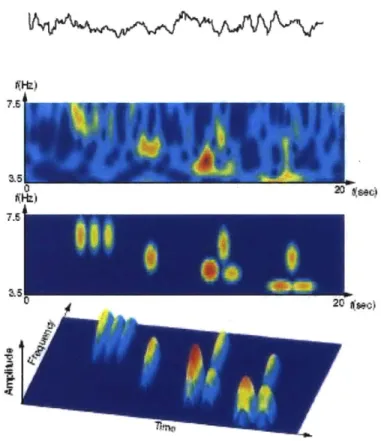
6-1 Bump modeling of EEG data . . . 153
6-2 Stochastic Event Synchrony: principle . . . 155
6-3 Bump modeling . . . 156
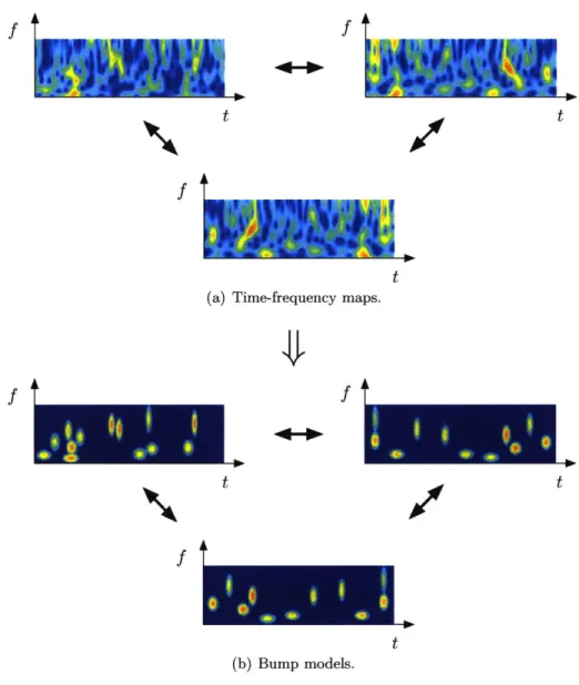
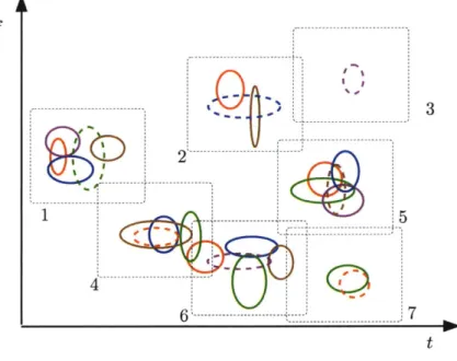
6-4 Multivariate SES: principle . . . 158
6-5 Generative model . . . 160
6-6 Classification with bivariate SES . . . 183
6-7 Classification with multivariate SES . . . 183
6-8 AD Classification with three features . . . 184
C-1 Bump modeling: principle . . . 201
C-2 EEG electrodes placement . . . 204
D-1 Box plots for the most discriminating classical measures . . . 210 11
List of Tables
Definitions
We use the following conventions and notations in this thesis: key concepts, when they are first introduced, are italicized. We will use the symbol = for equations which define symbols. The notation of single elements v of a set V uses a regular typeface, while the bold typeface v denotes vectors or arrays. For any set V, 2v denotes the set of all subsets of V.
A graph
9
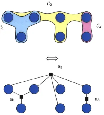
= (V, E) is an object composed of a finite set of nodes or vertices V and a set E of unordered pairs of elements of V. E denotes the set of oriented edges of (V, E) whose unoriented version belongs to E. More generally, a hypergraph (V, C) is composed of a set of nodes V and a set of hyperedges C C 2v, where each hyperedge C E C is anonempty subset of V. Finally, a network consists of a graph or hypergraph, along with a collection of functions indexed by the elements (nodes, edges, or hyperedges) of the graph or hypergraph.
Hypergraphs can be seen as being equivalent to factor graphs. A factor graph is a bipartite graph
9
= (G, E), with G = V U A, and where the vertices of V are calledvariable nodes and the vertices of A are called factor nodes. There is a trivial bijection between hypergraphs and graphs, where for any hypergraph (V, C), we create a factor graph (V, A, E), where each hyperedge C is mapped to a single factor node a(C) E A, and
we create edges in the factor graph according to the rule v E C if and only if (v, a(C)) E E.
Given a graph (V, E) (resp. hypergraph (V, A)) and a subset U of V, the graph (resp. hypergraph) induced by U is the graph (U, E') (resp. (U, C')), where E' = {(u, v) E E : u, v E U} (C' = {C E C : C c U}. Induced networks, which we call subnetworks, are
defined similarly.
C*
C3
a2
a1 a3
Figure 0-1: Equivalence between hypergraphs and factor graphs
a shortest path (in number of edges) between u and v. Given a node u and integer r > 0, let Bg(u, r) = {v E V : d(u, v) <; r}. Let also Ag(u) = B(u, 1)\{u}. The extended set of neighbors Af(u)e is Bg (u, 1) = K(u) U {u}. For any r > 0, let
NA/
(v) be the subnetwork induced by Bg(u, r). For any node u, Ag(u) A |Ng(u)I is the number of neighbors of u ing. Let Ag be the maximum degree of graph (V, E); namely, Ag = max, jg(v)|. Often we will omit the reference to the network
g
when obvious from context.We will often consider sets and sequences (i.e., ordered sets) of elements indexed by the vertices of a network (V, E). For any set or sequence of elements x = (x,)vey indexed by the elements of
a
set V, and any subset U = (v1,v2, . ,ViUi) of V, xU = (XVI, XV2, --. , oVV )denotes the sequence of corresponding elements. For any set or sequence x and element u
E V, we denote xu
= xv\{u} = (XV),ev,vsu the set of elements for all nodes other thanu. Finally, for any set or sequence x, and element u E V, we denote x, A XvEK(u) the set
of elements that are neighbors of u.
We will assume an underlying probability space, denoted as (Q, B, P). For a set of discrete random variables X = (X1,..., Xa) and possible outcome x = (x1,..., zX), we
denote P(X = x) the probability that the random vector X takes the value x. If the Xi are jointly continuous, we denote by dP(X = x) the density of X. Finally, for any random variable X, E[X] denotes the expected value of X, and for any sub-- algebra A of B, E[X
I
A] is the conditional expectation of X given A.For any finite set
X,
we denoteS(x)
the simplex overx,
or alternatively, the set of probability distributions over elements of X: S(x) = {x E [0, 1]X Va E X, x(a) > 0, andEaex
x(a) = 1}. Elements a of x can be viewed as elements of S(x) (with unit mass at a). For any 6 = 1/n > 0 for some positive integer n, let S6(X) be the set of prob-ability distributions over x whose components are integer multiples of3
(Vs E S6(x), ]k = (ki,..., k1)j) E NIXI such that s = 6k and Ti ki = 1/6).Introduction
Graphical Models
Many models of optimization, statistics, control, and learning capture local interactions and sparse dependencies by means of a network in which different components are con-nected and interacting. Originating in statistical physics under the name Ising model in the first half of the 20th century (see [Isi24, Ons39, Ons44]), these classes of mod-els have since flourished in a number of different fields, most prominently, statistics and artificial intelligence [Lau96, Jor98, WJ08], theoretical computer science and combinato-rial optimization [ASO4, BSS05, GNS06, BG06, BGK+07, GG09], coding theory [BGT93, MU07, RU08], game theory [KLS01a, OK03, DP06], and decentralized optimization and control [KPOO, GDKV03, RR03, CRVRL06]. While the problems these different commu-nities consider and the questions they aim to answer are at first glance different, research in recent years has uncovered previously unknown connections between these fields. At a high level, research in graphical models has aimed to understand how macroscopic phenom-ena of interest arise from local properties, and efforts to answer this question have led to the fast development of new classes of distributed algorithms designed to compute critical physical parameters of the system, perform optimization, or carry statistical inference on the network.
The basic model
The basic model we will be considering throughout this thesis is the following: we consider a team of agents working in a networked structure given as a hypergraph (V, A), where V is the set of agents, and where each hyperedge a E A represents local interaction within a subteam of agents. Each agent u E V makes a decision xu in a finite set X L {0, 1, ... , T
-1}. For every v E V (resp. every hyperedge a), a function
#:
:X3 R (resp.x
#a
: X al a R) is given. Functions#v
and Oa will be called potential functions and interaction functions respectively. Let <1 = ((#v)vEV, (#a)aEA). A vector x = (x 1, x2,- . . , XlV) of actions is calleda solutions for the decision network (individual components x, will be called decisions). The set
g
= (V, A, <D, X) is called a decision network or graphical model. The set of potential and interaction functions <D defines a network function (often called the energy function)Fg which associates with each solution x the value
Fg (x)
=S
#a(xa)
+
# (O )
(1)
aeA V
In an optimization context, the goal is to find a decision vector x* which minimizes or maximizes the function Fg (x): x* E argmaxxFg
(x).
In the context of statistics, the function Fg defines a family of probability distributions on decision vectors x. These distributions are called exponential family distributions, and are indexed by real parameters 6 = (6a)aCA called exponential parameters or canonical
parameters; the exponential family distribution with parameters 0 assigns to each solution x a probability
P(x) = Z(6) exp OaEa(xa)) (2)
where
Z(0)
A
exp(
a9a(Xa))(3)
X acA
The quantity Z(9) is called the partition function of the network
g,
and F(O) = log(Z(6)) is called the log-partition function or cumulant function.An important special case is when Oa = -# for all a E A. The resulting distribution is called the Gibbs distribution (also known as Boltzmann distribution) and the parameter
#
is then called inverse temperature, in analogy with the Boltzmann equation from statistical physics. For a Gibbs distribution, the log-partition function F(#) is also called the free energy of the system.Frameworks, examples, and applications
Let us mention a few example of models from different fields which can be cast as special cases of graphical models, and consider the key problems each field focuses on.
As an example, common models in the area of statistical inference are Bayesian net-works and Markov Random Fields (MRF) (see [Lau96, WJ08] for a more in-depth presen-tation of these topics). A Markov Random Field is a probability distribution on a set of random variables (X1, X2, ... , Xn) E x" such that the joint probability distribution takes
the form
P(X) =0 c(Xc) (4)
CEcl(V,E)
where (V, E) is a graph, cl(V, E) is the set of cliques (complete subgraphs) of (V, E), and for each clique C, 'bc is a nonnegative function. Markov Random Fields constitute a generalization of Markov chains, which can be seen as one-dimensional, directed MRFs. In a similar fashion to Markov chains, Markov Random Fields satisfy a collection of conditional independence relations, and can be proven to model any set of consistent independence relations, explaining their power as modeling tools. A Bayesian network is defined on a
directed acyclic graph (DAG) (V, E) and defines a joint probability distribution
P(X) =
P(XvI
Xp(V)) (5)vEV
where V is the set of nodes of the DAG (V, E), and for each V, P(v) denotes the set of par-ents of v in V, E. Morever, for any assignment of variables XP(v), p(xv I £p(v)) is a discrete probability distribution on x,. Because they are defined on a directed graph, Bayesian networks are extensively used in systems where causality links between variables are of interest. As mentioned, one can easily show [WJ08] that both Markov Random Fields and Bayesian nets can be modeled as graphical models. The main research problems pertaining to MRFs and Bayesian nets are as follows. In many cases, the variables of an MRF or Bayesian net can be divided in three categories: variables which are observed (observed variables), variables which are unobserved and which are not of direct interest (structural variables), and variables which we would like to predict given the information provided by the observed variables (target variables). The key mathematical step then consists in marginalizing the structural variables in the models described by equations (4) and (5),
in order to obtain the conditional distribution of the target variables given the observed variables. Another key object in such a model is the state which achieves the mode of the density, namely, the state which maximizes the a priori likelihood.
Other examples can be found in the field of combinatorial optimization, where the problem of interest can often be described as that of finding subsets of nodes or edges which satisfy various constraints supported by the underlying graphs. Examples include independent sets, matchings, k-SAT, graph coloring problems, and many others. Often, the goal is to identify which of these objects minimizes or maximizes some objective function. The search space is typically exponentially large, and so is the number of local minima, making such an optimization task hard. Again, it can be shown that many such optimiza-tion problems can be converted into an optimizaoptimiza-tion problem in a graphical model (see Chapter 4 for the concrete example of Maximum Independent Set). Other problems of interest involve counting the number of solutions which satisfy the constraints, or at least estimating the rate at which this number grows when the size of some structured graph grows as well. Both of these problems can be directly related to the issue of computing the partition function of a graphical model.
Finally, in statistical physics, the Ising model [Tal03] with interaction energy J is described by set of particles s positioned on a lattice (V, E), each of which can be in one of two spin states (s E {-1, +1}). In this case, the total energy of the system is given by Fg(s) = - (uv)EE Jss, and the corresponding Boltzmann distribution is
P(s)
=exp (0
Jsis3)
(6)
(u,v)EE
where
#
is the inverse temperature. An important object of interest in this model is the ground state - a state which achieves the minimum possible energy, i.e., corresponds to the minimum of Fg(s). For J < 0, this is equivalent to the problem of finding the so-called max-cut of a graph.Computational complexity and randomness
Looking at all the examples above, research in graphical models can be seen as trying to address two categories of problems.
The first category includes counting and sampling problems. Counting involves com-puting (exactly or approximately) the partition function Z(0), or equivalently, the free energy F(0). Sampling involves sampling a set of variables according to the Gibbs dis-tribution for a given i. A related task include computing or sampling from the marginal Gibbs distribution for a given variable (or a small number of variables). In a wide num-ber of frameworks, counting and sampling can be shown to be problems of equivalent computational complexity [JVV86].
The second category regards optimization. Here the objective is to identify a vector x which minimizes or maximizes the energy function Fg(x). Many hard constraints can be modeled by making infeasible configurations have infinite positive (or negative) energy.
In many cases of interest, the combinatorial nature of the problems considered im-plies that optimization or inference on these models is hard, even when using algorithms that take advantage of the underlying graphical structure [Coo90, Rot96, CSH08]. Ex-act inference in most graphical models is NP-hard, counting the number of solutions of many combinatorial problems on a graph is P-hard [Jer03], and finding an optimal policy for a Markov Decision Process takes exponential time and space in the dimension of the state-space, even for very simple factored Markov Decision Processes [PT87, BTOO]. Thus, approximate methods to find solutions that theoretically or empirically achieve proximity to optimality are needed.
Optimization methods and message-passing schemes
The search for approximate methods typically differs from field to field. In combinatorial optimization the focus has been on developing methods that achieve some provably guar-anteed approximation level using a variety of approaches, including linear programming, semi-definite relaxations and purely combinatorial methods [Hoc97]. In the area of graph-ical models, researchers have been developing new families of inference algorithms, one of the most prominent being message-passing algorithms.
At a high level, message-passing schemes function as follows. For each directed edge e = (u - v) of the graph, a message yu is defined, usually a real number, a vector of
real numbers, or a function. Each node of the graph receives messages from its neighbors, combines them in some particular way, and computes new messages that it sends back to its neighbors. The passing of messages in the network is either performed synchronously or asynchronously, and upon convergence (if the scheme converges), all incoming messages to a node u are combined in order to compute either a decision x or a marginal distribution P(XU).
One of the most studied message-passing algorithms is the Belief Propagation (BP) algorithm, [Lau96, Jor04, YFWOO]. The BP algorithm is designed both for solving the problem of finding the optimal state using the max-product version, as well as for the prob-lem of computing the partition function, using the sum-product version. The BP algorithm is known to find an optimal solution x* when the underlying graph is a tree, but may fail to converge, let alone produce optimal solutions, when the underlying graph contains cycles. Despite this fact, it often has excellent empirical performance [FM98, YMW06,
WYM07].
Moreover, it is a distributed algorithm and easy to implement. This justifies the wide applicability of BP in practice and the intense focus on it by the researchers in the signal processing and artificial intelligence communities. Nevertheless, a major research effort has been devoted to developing corrected version of Belief Propagation, and to understanding the performance of message-passing schemes.
This thesis focuses on developing a new message-passing style algorithm, the cavity expansion algorithm, and to understand and study its performance in the context of large-scale graphical models, with emphasis on the question of how randomness affects the com-plexity of optimizing in a graph. In particular, we put ourselves in a framework where the potential and edge functions are randomly generated, and try to understand under which conditions a problem is computationally hard or easy. These conditions typically relate to the structure of the graph considered, along with the distribution of the cost functions. The connections which have been uncovered between statistical physics and optimization can be of much help in this respect. Of particular interest is the study of a statistical physics phenomenon known as the correlation decay property. At a high level, correlation decay indicates a situation in which the "influence" of a node on another node of the network decreases quickly as the distance between them grows. We show that, in many cases, the onset of correlation decay often implies that the optimization problem becomes easy on average.
Organization of the thesis and contributions
Chapter 1: Message-passing schemes and Belief Propagation
In the first chapter, we present our general optimization framework, and give a short introduction to message-passing algorithms, Belief Propagation, and some of the most prominent message-passing variations that were designed to address issues of correctness or convergence of BP.
Chapter 2: The Cavity Expansion algorithm
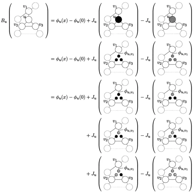
In the second chapter, we propose a new message-passing-like algorithm for the problem of finding x* E argmax Fg(x), which we call the Cavity Expansion (CE) algorithm. Our algorithm draws upon several recent ideas, and relies on a technique used in recent de-terministic approximate counting algorithms. It was recently recently shown in [Wei06] and [BG06] that a counting problem on a general graph can be reduced to a counting problem on a related self-avoiding exponential size tree. Following a generalization of this technique later developed in [GK07b, BGK+07], we extend the approach to general opti-mization problems. We do not explicitly use the self-avoiding tree construction, and opt instead for a simpler notion of recursive cavity approximation. The description of the CE algorithm begins by introducing a cavity Bv(x) for each node/decision pair (v, x). B,(x) is defined as the difference between the optimal reward for the entire network when the action in v is x versus the optimal reward when the action in the same node is 0. It is easily shown that knowing Bv(x) is equivalent to solving the original decision problem.
Our main contribution is to obtain a recursion expressing the cavity Bv(x) in terms of cavities of the neighbors of v in suitably modified sub-networks of the underlying network. From this recursion, we develop the CE algorithm, which proceeds by expanding this recursion in the breadth-first search manner for some designed number of steps t, thus constructing an associated computation tree with depth t. We analyze the computational effort and prove it is exponential in t. We therefore need conditions which guarantee that using the cavity recursion for small t results in near-optimal decisions, which is the object of the following chapters.
Chapter 3: Correlation decay and efficient decentralized optimization in
decision networks with random objective functions
In the third chapter, we investigate the connection between a property of random systems, called the correlation decay property, and the existence of polynomial-time, decentralized algorithms for optimization in graphical models with discrete variables and random cost functions.
A key insight of this thesis is that in many cases, the dependence of the cavity B,(x) on cavities associated with other nodes in the computation tree dies out exponentially fast as a function of the distance between the nodes. This phenomenon is generally called correlation decay and was studied for regular, locally tree-like graphs in [GNS06].
It is then reasonable to expect that the Cavity Expansion algorithm and the correlation decay analysis can be merged in some way. Namely, optimization problems with general graphs and random costs can be solved approximately by constructing a computation tree and proving the correlation decay property on it. This is precisely our approach: we show that the correlation decay property is a sufficient condition which guarantees the near optimality of the CE algorithm. Thus, the main associated technical goal is establishing
the correlation decay property for the associated computation tree.
We indeed establish that the correlation decay property holds for several classes of decision networks associated with random reward functions <D =(
#&, #5,).
We provide a general technique to compute conditions on the parameters of families of distribution that ensure that the system exhibits the correlation decay property. We illustrate the applicability of the method by giving concrete results for the cases of uniform and Gaussian distributed functions in networks with bounded connectivity (i.e., bounded graph degree).Chapter 4: Connections between correlation decay and computational
hardness of probabilistic combinatorial optimization
In the fourth chapter, we look at similar questions for a specific combinatorial optimiza-tion problem, namely, the Maximum Weight Independent Set (MWIS). We show how the CE algorithm applies to the MWIS problem and provides conditions under which the CE algorithm finds an approximately optimal solution. The application of CE in a randomized setting has a particularly interesting implication for the theory of average case analysis of combinatorial optimization. Unlike some other NP-complete problems, finding a MWIS of a graph does not admit a constant factor approximation algorithm for general graphs.
We show that when the graph has maximum degree 3 and when the nodes are weighted independently with exponentially distributed weights, the problem of finding the maxi-mum weighted independent set admits a polynomial time algorithm for approximating the optimal solution within 1 + e for every constant E > 0. We also provide a generalization
for higher degrees, and detail a framework for analyzing the correlation decay property for arbitrary distributions, via a phase-type distribution approximation. Thus, surpris-ingly, introducing random weights translates a combinatorially intractable problem into a tractable one. We note that the sufficient condition pertains only to the weight distribution and the degree of the graph. As such, CE does not suffer from the loopiness of the graph being considered, a very uncommon feature for a message-passing style algorithm. We also provide partial converse results, showing that even under a random cost assumption, it is NP-hard to compute the MWIS of a graph with sufficiently large degree.
Chapter 5: Correlation Decay in graphical games
Graphical games [KLS01a] are a natural extension of the discrete optimization graphical models of Chapter 1, where each agent is assigned her own family of cost functions which she tries to optimize while taking into account other agents' potentially conflicting ob-jectives. It is well known that computing the Nash equilibrium of a game is hard, (see Daskalakis et al. [DGP09]), even when considering sparse networks. These facts arguably make NE an unlikely explanation for people's or markets' behaviors. Thus, there has thus been an interest in adapting message-passing algorithms to the computation of Nash Equi-libria, under the reasoning that simple distributed schemes might better represent social computation. In [KLS01a), and then [0K03], Kearns et al. develop Nash Propagation, an analog of Belief Propagation for the setting of graphical games. Like BP, NP is optimal or near-optimal for tree-structured games.
Our objective is two-fold. First, we develop a general framework for designing message-passing algorithms for graphical games. These message-message-passing algorithms aim to compute so-called Nash cavity functions, which are local constraints encoding as much of the global Nash equilibrium constraints as possible. With the help of this framework, we develop the Nash Cavity Algorithm, a general message-passing heuristic which aims to try to compute Nash cavity functions for general graphical games. In particular, we show that TreeProp is a special case of the Nash Cavity algorithm for graphical games on tree.
games on trees, and show that, under appropriate conditions, the Nash cavity functions of games exhibiting the correlation decay property can be computed locally.
Chapter 6: Application of graphical models and message-passing
tech-niques to the early diagnosis of Alzheimer's disease
In the last chapter, we consider a particular application of graphical models and message-passing algorithms. The problem in question is a statistical signal processing problem, specifically, measuring the similarity of a collection of N point processes in RA. The work is motivated by the following application: developing a new measure of synchronicity between different parts of the brain, as recorded by electroencephalogram electrodes, and using said measure to give an early prediction of Alzheimer's disease. We show that the resulting measure of synchronicity outperforms a vast number of other EEG-based measures in the task of predicting the onset of Alzheimer's disease.
Chapter 1
Message-passing schemes and
Belief Propagation
1.1
Introduction and literature review
Foundations of message-passing algorithms
In this chapter, we present the Belief Propagation (BP) algorithm, arguably the first, simplest, and most commonly used form of message-passing algorithms. Introduced by Pearl in the context of inference in probabilistic Al [Pea82, PS88, PeaOO], the sum-product algorithm enabled distributed computation of marginal probabilities in belief networks, and its success encouraged the shift from classical to probabilistic Al. BP was later extended to max-product (min-sum in the log domain), a version of BP which computes the mode of the distribution underlying a Bayesian Network. Belief Propagation was then proven to output the correct solution when the graph is a tree (or a forest), and initially, most research effort in message-passing for Al focused on algebraic, exact generalizations of BP to graphs with cycles [Lau96].
Eventually, it was discovered that Belief Propagation, even when applied to graphs with cycles (the idea is referred to as "loopy Belief Propagation"), often had excellent empirical performance [FM98]. This surprising discovery fostered much research activity in the do-main of message-passing algorithms, leading to the development of several new distributed computation techniques, and revealing connections between classical optimization (most prominently convex optimization and linear programming relaxations) and message-passing
methods [BBCZ07, WYM07, YMW06, WJ08, SSW08].
Much earlier, Gallager, in his 1960 PhD thesis [Gal60, Gal63], invented a new class of error-correcting techniques called Low Density Parity Check (LDPC) codes, along with an iterative algorithm to perform decoding of LDPC codes. This early algorithm was later found to be an early version of Belief Propagation. Similar iterative algorithms performing on graphs were later investigated by researchers in coding theory, in particu-lar Forney [FJ70], Tanner [Tan8l], Battail [Bat89], Hagenauer and Hoeher [HH89], and finally Berrou and Glavieux [BGT93], whose BP-like turbocodes nearly attained the Shan-non capacity. The performance of turbocodes sparked great interest in message-passing algorithms in the coding theory community, see for instance later work by Kschischang, Frey, Loeliger, Vontobel, Richardson, Urbanke, and many others [DMU04, LETB04, VK05, LDH-07, MU07, RU08].
Finally, a new class of models for magnetized particles with frustrated interations, spin glasses, generated a lot of interest in the statistical physics community in the late 1980s, especially after Parisi solved a particular Ising model proposed by Sherrington and Kirk-patrick [SK75] a decade before. Parisi's technique (see [MPV87]), the cavity method, bore a lot of similarities to Belief Propagation, and was found to have connections to combinato-rial optimization problems such as k-SAT or graph coloring. This result was one example of the convergence of interests between statistical physics, mathematics (combinatorics especially), computer science (computational complexity) and Al.
On the one hand, physicists started to study combinatorial optimization problem in order to both understand better the relations between computational hardness and ran-domness (in particular, through the study of phase transitions), and to develop stronger algorithms for solving constraint satisfaction problems. Some of the algorithms developed, such as survey propagation, proved to solve very efficiently large instances of hard problems (see for instance [BMZ05]).
On the other hand, mathematicians investigated, formalized, and made rigorous tech-niques and problems from statistical physics. Of particular interest is the solution of the ((2) Parisi conjecture for the random minimal assignment problem (see [Ald92, Ald0l, AS03]). One of the key ideas was the study of fixed points of recursive distributional equa-tions (RDE) (see Chapter 4). Again, the existence and convergence to a fixed point of a RDE can also be understood in terms of asymptotic convergence of the Belief Propagation algorithm in an infinite random graph.
particular, can therefore truly be seen to be at the intersection of many different fields: Al, coding and information theory, statistical physics, probabilistic combinatorics, and computational complexity (see [WJ08) for an overview of inference techniques in graphical models and [HW05, MM08] for comprehensive studies of the relations between statistical physics, statistical inference, and combinatorial optimization).
Each of these brings a different point of view on the mechanics and performance of Belief Propagation, and, based on those particular insights, offers particular generalizations or corrections of Belief Propagation.
Modern work on Belief Propagation
The empirical success of Belief Propagation, despite the fact that BP is a nonexact recur-sion, prompts the following two questions. First, can one identify problems and conditions under which BP is provably optimal, and second, can one design a "corrected" version of BP, which will achieve greater theoretical and practical performance, specifically for the cases where BP is proven not to work?
Regarding the first question, researchers have recently identified a number of frame-works in which BP converges to the optimal solution, even if the underlying graph is not a tree. In a framework similar to ours, Moallemi and Van Roy [MR09] show that BP con-verges and produces an optimal solution when the action space is continuous and the cost functions are quadratic, convex. More generally, when these functions are simply convex, the authors exhibit in [MR07] a sufficient condition (more specifically, a certain diagonal dominance condition) for the convergence and optimality of BP. Other cases where BP pro-duces optimal solutions include Maximum Weighted Matchings [San07, BBCZ08, BSSO8], Maximum Weighted Independent Sets if the LP relaxation is tight [SSW08], network flows [GSW09], and, more generally, optimization problems with totally unimodular con-straint matrices [Che08]. Furthermore, in the case of Gaussian Markov Random Fields, sufficient conditions for convergence and correctness of Belief Propagation were studied in [RR01, CJW08, JMW06, MJW06]. Finally, a number of researchers have investigated sufficient conditions for BP to converge (to potentially suboptimal solutions), and then tried to quantify the resulting error of the solution obtained; see for instance [Wei00, TJ02, MK05, IFW06).
Regarding the second question, over the last few years, many corrected or improved ver-sions of BP have been proposed, most notably the junction tree algorithm [Lau96], survey propagation [MMW07], Kikuchi approximation-based BP and generalized Belief Propa-gation (GBP) [YFWOO], tree-reweighted Belief PropaPropa-gation [WJW03b, WJW05a, KW05, Kol06], loop-corrected Belief Propagation [MWKR07), loop calculus [CC06a, CC06b], and dual LP-based Belief Propagation algorithms [SMG+08b, SGJ08, SJ09]. Each of these algorithms differs in its conditions for convergence or optimality, running time, or the type of bounds provided on the free energy of the system considered.
In this chapter, we present the Belief Propagation algorithm (optimization version), along with some of the most prominent message-passing algorithms which aim to correct BP for the problems in which it performs poorly.
1.2
Message-passing schemes and framework
Let us for convenience restate the model we previously introduced. We consider a pairwise decision network
g
= (V, E, <b, X). Here (V, E) is an undirected graph without repeated edges, in which each node u E V represents an agent, and edges eE
E represent a possible interaction between two agents. Each agent makes a decision xu E X -{0,
1,... , T - 1).For every v E V, a function
#,
: X -+ R is given. Also for every edge e = (u, v) a function#e
: X2 -+ R is given. Functions#v
and#e
will be called potential functions and interaction functions respectively. Note that in general, we don't require the presence of potential functions, as these can be absorbed into the interaction functions as follows: for any potential function#,,
corresponding to a node u E V, choose an arbitrary neighborv of u, and update
#u
and#uv
into#'
and#$,
as follows:#'(x)
= 0 for all x, and #,V(XU, X) = #2,x(u, zV) + #U(XU) for all xu, x. Let <D = ((#v)VE, (#e)eEE). The object9 = (V, E, D, x) will be called a pairwise decision network, or pairwise graphical model.
A vector x = (XI, x2,..., XIVi) of actions is called a solution for the decision network. The value of solution x is defined to be Fg(x) =
E(u,v)EE
#UV
u, IXV) + ov Ov (xo). Thequantity Jg A maxx Fg(x) is called the (optimal) value of the network
g.
A decision x is optimal if Fg(x) = Jg. Our objective is to compute an optimal (or near-optimal) solutionfor the network:
Given a network
G
= (V, E, (#v)veV, (#U,V)(U,v)EE), X),find
x* E xV such thatx*
E
argmaxx- EOV(xv)+
OU'( Xz))\V u,v
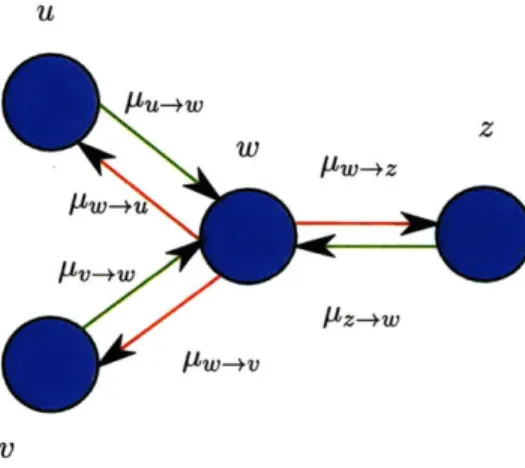
Message-passing schemes are a simple, naturally distributed, and modular class of algo-rithms for performing optimization in graphical models. They function as follows: we define a vector of messages M E SE, where S is the space of messages (often, S = R). Given some understanding of the optimization problem at hand, we design for each ori-ented edge e = (u -+ v) a function Fusv : S -+u S, and we iteratively update the vector
M by the following operation:
V(u -+ v) E E, Mu-e = Fu_,v(My,-2) (1.1)
In other words, messages outgoing from u are functions of message incoming to u (see Fig. 1.2). Assuming the scheme converges, we set the variable xu to gu(Mgru) for some carefully chosen function gu: the decision xu of u is a function of messages incoming to u in steady state.
Because of the recursions we consider have their root in dynamic programming, in the following, it will be more natural for us to denote pLav, the message sent from u to v, by pv<u, message received by v from u (these two notions being identical in our context).
U
V
-Figure 1-1: A message-passing scheme
1.3
The Belief Propagation algorithm
In this section, we derive the Belief Propagation equations by proceeding in two steps. First, we develop a recursion where variables are located on the nodes of our network
g.
This recursion is natural and based on a simple dynamic optimization principle, but is not easily parallelizable, nor easily applied to general (non tree) graphs. In the second step, we show how the dynamic optimization equations can be converted into a new set of recursive equations, where this time variables dwell on the edges of the graph. This new set of equations constituting the Belief Propagation equations, are naturally parallelizable, and are easily applied to arbitrary graphs (albeit non optimally). We begin by introducing useful notations.
Given a subset of nodes v = (v1,... O), and x = (x1,... xk) E yk, let Jg,v(x) be the optimal value when the actions of nodes vi, ... , V are fixed to be x1,... , Xk respectively:
Jg,v(x) = maXx:xv=x,1<i<k Fg(x). Given v E V and x c x, the quantity Bg,v(x) =
Jg,v(x) - Jg,v(0) is called the cavity of action x at node v. Namely it is the difference of optimal values when the decision at node v is set to x and 0 respectively (the choice of 0 is arbitrary). The cavity function of v is Bg,v = (Bg,v(x))XEX. Since Bg,v(O) = 0, Bg,v can be thought of as element of RT-1. In the important special case x = {0, 1}, the cavity function is a scalar Bg,v = Jg,v(1) - Jg,v(0). In this case, if Bg,v > 0 (resp. Bg,v < 0) then Jg,v(1) > Jg,v(0) and action 1 (resp. action 0) is optimal for v. When Bg,v = 0 there are
optimal decisions consistent both with xv = 0 and x, = 1. When
g
is obvious from the context, it will be omitted from the notation.Vertex-based dynamic optimization
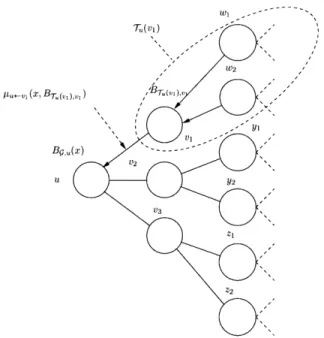
Given a decision network G = (V, E, <, X) suppose that (V, E) is a tree T, and arbitrarily root the tree at a given node u. Using the graph orientation induced by the choice of u as a root (i.e., children of a node v are further from u than v is), let Ca(v) denote the set of children of any node v in (V, E), and let Tu(v) be defined as the subtree rooted in node v. In particular, G = T (u). Given any two neighbors v, w E V, and an arbitrary vector B = (B(x), x E X), define
Pv<-w(x, B) = max(#v,,(x, y) + B(y)) - max(#v,w(0, y) + B(y)) (1.2)
W11
11u+-v1 (X, BT (i, ) (- 1
V22
V3
2
Figure 1-2: Dynamic optimization recursion on a tree
for every action x E X. p is called the partial cavity function.
Proposition 1 (Cavity recursion for trees). For every v E V and x E x,
BT (v),v(x) = #v(x) - #v(0) + (v (1.3)
Proof. Suppose KIC(v) = {wi, ... , wd}. Observe that the subtrees T(wi), 1 < i < d, are disconnected (see Fig. 1.3). Thus,
d
Bziv),v(x) = 4(x) + ax v,wj (x, xj) + JrTu(w),w,(xj )
j=1 d
- #v (0) - max #: 0Vw, (0, xy) + JT (w,),w (xj))}
+
max
(#v,ax
(x,
y)
+
JT(w),w, (y))
-
max
(#v,wj (0,
j=1
y) + JT (w,),w,(y))}
For every
j,
max
(#eWj
(x, y) + JT(w),w, (y)) - max(#,wj
(0, y) + JT(wj),wj (y))max (#v,wi (x, y) + JKT(wj),wj () - JT (w),wj (0)) - max (#uvi (0, y) + JET (wm),w (Y) - JTU (w),wj (0))
The quantity above is exactly pvWj (x, BT,(wj),w,). E
By analogy with the algorithm we develop in the next chapter, Equation 1.3 will be called the cavity recursion for trees. It is based on nonserial dynamic optimization [BB72], which computes value functions of subtrees of the original graph. In the equations above, the variables of interest are cavities, and they are computed at the nodes of the graph.
Edge-based Belief Propagation
We now transform equation 1.3 into an equivalent system of equations where the variables are computed on oriented edges of the graph. Recall that since
g
is a tree, for any two nodes v, w, removing the edge (v, w) from the graph (V, E) separates it into two trees, one containing v, the other containing w. We denote the one which contains v (resp. w) T,<_, (resp. T<,). For any edge (v, w), letg,
be the network induced by v-_w U {v, w}, with the additional modification that the potential#v
is removed from that network. Finally, let Mvew(xz) denote Bgv,,(xv). Since v has a unique neighbor w in gv , it is easy to check that we haveMv, (xv) = pv_(xv, BTv,.,v) (1.4)
Proposition 2 (Belief Propagation). For all u E
9,
Bg,u(xu) =
#U(xU)
-#(0)
+
E3 M<_V(X) (1.5)vc~K(u)
For all (u, v) E E,
Mw<_V(xU) = p><_3 x (#v + Mv<_.W) (1.6)
Figure 1-3: Tree splitting Tree T split into , and T__
Proof. For the first equation, consider Equation (1.3) for v = u, and note that K(u) = Af(u), and as noted previously, Tu(u) = g. We obtain
Bg,u(xU) = U(x) - #2(0) +
Z
/W<_v(x, BT(v),v)vEK(u)
Since clearly T<_v = Tu(v), Equation (1.4) implies that Bg,u(x) = #U(x) - #k(O) +
ZVEN(U) Mu<_V(z.), and thus finishes the proof of the first equation. The second equation follows from the exact same principles and the observation that for a node v with neighbors
(u,i, .-. , wd}, T(wi) is equal to <,, for all i. l
Equations (1.5) and (1.6) are called belief propagation equations, and make the prac-ticality of the BP algorithm apparent. Indeed, Equation (1.6) can be seen to be iterative in nature, since it writes the set of all messages (Muz_) - as a function of itself.
(U<-V)E E
This naturally suggests the following iterative scheme to compute the Muv: for any
(u +- v) E E, xu E X, and r > 0
M +(xu) = Azu+-V wU Mviw (XV) (1.7)
WENr(v)\{u}
where the values MUO+_, are initialized to arbitrary values. While it is not necessarily obvious that this scheme converges for trees, it can easily be shown by induction that for r greater
than the depth of tree, the messages M[', are in fact stationary and equal to their correct values Muz_. This subsequently allows the use of Equation (1.5) to compute the cavities, and therefore the optimal solution. In that sense, Proposition 2 is the restatement of the well-known fact that BP finds an optimal solution on a tree [MM08]. More importantly, unlike Equation (1.3), the algebraic structure of Equation (1.7) does not require that the graph be a tree, and can therefore be applied to any general graph. The resulting algorithm is called loopy Belief Propagation. As mentioned previously, it may now not converge, and even if it does, plugging the obtained messages into Equation (1.5) may result in an arbitrarily poor solution.
Generalization to factor graphs
We now generalize the Belief Propagation equations to hypergraphs. As for the pairwise case, we will first derive dynamic optimization equations, and then rewrite them as message-passing equations in a factor graph. Consider a factor graph (V, A, E, <D, x), for which the underlying network (V, A, E) is a tree T, and arbitrarily root the tree at a given node u E V. Again, denote 'T(v) the subtree rooted at v E V U A when using the orientation
induced by u as root, and Ku(v) the children of v. Note that for any v E V, K2u(v) C A,
and for any a E A, K(a) C V. Finally, consider any v E V and a E Eu (v), and denote ka = Ku(a) the number of children of a; for any x, E x, and an arbitrary function M from
xka to R, define the partial cavity function (for factor graphs) pu<a as
pv<-a(X, B) = max (a(X, Yi, Y2, Yka) + M(yi, ... yka))
The analog of the recursion (1.3) for factor graphs is as follows (the proof is essentially identical to that of Proposition 1):
Proposition 3. For every v E V and x E X,
BT (,),v(x) = #v(x) - #$ (O) + / pv<-a(x,
(
BT(w),w) (1.9)aeJC(v) weKu(a)
We now proceed to convert Equation (1.9) to a set of recursive equations on messages in the factor graphs. Once again, we use similar notations to the bipartite case: for any two neighbors v E V, a E A, removing the edge (v, a) separates T into two trees. _