Lévy Flights and Fractal Modeling of Internet Traffic
György Terdik and Tibor Gyires, Member, IEEE
Abstract—The relation between burstiness and self-similarity
of network traffic was identified in numerous papers in the past decade. These papers suggested that the widely used Poisson based models were not suitable for modeling bursty, local-area and wide-area network traffic. Poisson models were abandoned as unrealistic and simplistic characterizations of network traffic. Recent papers have challenged the accuracy of these results in today’s networks. Authors of these papers believe that it is time to reexamine the Poisson traffic assumption. The explanation is that as the amount of Internet traffic grows dramatically, any irregularity of the network traffic, such as burstiness, might cancel out because of the huge number of different multiplexed flows. Some of these results are based on analyses of particular OC48 Internet backbone connections and other historical traffic traces. We analyzed the same traffic traces and applied new methods to characterize them in terms of packet interarrival times and packet lengths. The major contribution of the paper is the application of two new analytical methods. We apply the theory of smoothly truncated Levy flights and the linear fractal model in examining the variability of Internet traffic from self-similar to Poisson. The paper demonstrates that the series of interarrival times is still close to a self-similar process, but the burstiness of the packet lengths decreases significantly compared to earlier traces.
Index Terms—Burstiness, fractal modelling, Lévy flights,
long-range dependence, network traffic.
I. INTRODUCTION
D
URING the 1990s, measurements of local-area network traffic [19] and wide-area network traffic [20] have proved that the widely used Markovian process models could not be applied for characterization of network traffic. If the traffic was Markovian process, the traffic’s burst length would be smoothed by averaging over a long time scale, which contradicted with the observations of the traffic characteristics at that time. Measure-ments of real network traffic of the last decade also confirmed [1] that traffic burstiness was present on a wide range of time scales. Traffic that is bursty on many or all time scales can be characterized statistically using the concept of self-similarity. Self-similarity is often associated with objects in fractal geom-etry—objects that appear to look alike regardless of the scale at which they are viewed. In case of stochastic processes, like time series, the term self-similarity refers to the process’ distri-bution remaining the same when viewed at varying time scales. Self-similar time series have noticeable bursts of long periods with extremely high values on all time scales. Characteristics ofManuscript received December 08, 2006; revised June 21, 2007; approved by IEEE/ACM TRANSACTIONS ONNETWORKINGEditor P. Nain. First published June 20, 2008; current version published February 19, 2009. This work was supported in part by the Hungarian NSF OTKA No. T047067.
G. Terdik is with the Faculty of Computer Science, University of Debrecen, Debrecen 4032, Hungary (e-mail: terdik@delfin.unideb.hu).
T. Gyires is with the School of Information Technology, Illinois State Uni-versity, Normal, IL 61790-5150 USA (e-mail: tbgyires@ilstu.edu).
Digital Object Identifier 10.1109/TNET.2008.925630
network traffic, such as packets/second, bytes/second, or length of frames, can be considered as stochastic time series. There-fore, measuring traffic burstiness is the same as characterizing the self-similarity of the corresponding time series.
The self-similarity of network traffic was observed in nu-merous papers, such as [2], [21], [24] and [6]. These and other papers showed that packet loss, buffer utilization, and response time were totally different when simulations used either real traffic data or synthetic data that included self-similarity [7], [8]. Recent papers challenge the applicability of these papers’ re-sults for today’s network traffic. For instance, the authors in [15] believe that it is time to reexamine the Poisson traffic as-sumption in the Internet backbone. They claim that traditional Poisson models can be used again to represent the characteris-tics of the aggregate traffic flow of multiplexed large numbers of independent sources [16], [31]. Their explanation is that as the amount of Internet traffic grows dramatically following the changes of network-technology, any peculiarities of the network traffic, such as burstiness, might cancel out as a result of the huge number of different multiplexed flows. The paper reports the analyses of current and historical traces of the Internet back-bone. The authors found that packet arrivals appeared Poisson at sub-second time scales, the traffic appeared nonstationary at multi-second time scales, and the traffic exhibited long-range dependence at scales of seconds and above.
Many previous works also analyzed the burstiness and the correlation structure of Internet traffic in various time scales in terms of the protocol mechanisms of the TCP, such as timeouts, congestion avoidance, self-clocking, etc. The authors of the paper [3] used a wavelet-based multiresolution tool to analyze the scaling behavior of Internet traffic on short time scales. This paper was one of the first works showing evidence that Internet traffic could be modeled using a multifractal model. The paper [4] demonstrated that scaling behavior of Internet traffic in short time scales can be explained by the closed-loop flow control of TCP and that the cutoff between short and long scale behavior is the round-trip-time of the TCP transfers. The paper [9] illustrated that short time scale burstiness is independent of the TCP flow arrival process and showed that in networks with light traffic, correlations across different flows did not have an effect on the short scale burstiness. The same authors illustrated in [10] that a Poisson cluster process could model the aggregate traffic where the packet interarrivals within individual clusters of each flow could be characterized by an overdispersed Gamma distribution. At the same time, the flow volumes showed heavy-tailed properties. Internet traffic was classified in alpha and beta flows in the paper [28]. It was shown that large transfers over high-capacity links, called alpha flows, produced non-Gaussian traffic, while the beta flows, low-volume transmissions, produced Gaussian and long-range dependent traffic. Long sequence of back-to-back packets can
cause significant correlations in short time scales. The reasons of sending long back-to-back packets in TCP or UDP sources were analyzed in [13], such as UDP message segmentation, TCP slow start, lost ACKs, etc. The same authors in [14] identified the actual protocol mechanisms that were responsible for creating bursty traffic in small time scales. It was shown that TCP self-clocking could shape the packet interarrivals of a TCP connection in a two-level ON-OFF pattern. The pattern causes burstiness in time scales up to the round-trip time of the TCP connection. The paper also investigated the effect of the aggregation of packet flows. The authors found that the aggregated packet flows did not converge to a Poisson stream, contradicting previous results. The authors argued that the burstiness could be significantly reduced by TCP pacing; selecting a 1-ms timer would make the traffic almost as smooth as a Poisson stream in sub-round-trip-time scales, contradicting the results in [15].
Our paper is motivated by the findings of [15]. We analyze the same traffic traces and applied our methods to characterize them. We are characterizing the network traffic traces as two time series, one is the arrival times of the packets and the other is the packet length in bytes. These two series are different in nature. The arrival times form a monotone increasing series. The differences between two consecutive times, called inter-arrival times, are independent, identically distributed random variables. The classical modeling of the interarrival times goes back to Erlang, who successfully modeled the phone calls by a Poisson process with interarrival times distributed exponen-tially. We generalize his model by changing the distribution to a general family of infinitely divisible distributions and by the cor-responding Lévy processes [29]. Obviously, we are only inter-ested in distributions that are totally concentrated on the positive half-line. Since a subset of these distributions—called -stable distributions (asymmetrical in our case)—provides self-similar processes, we are able to examine if our traces are self-similar, and more significantly, how close they are to being self-similar. The instrument of our analysis is the so called Truncated Lévy Flights [35].
The series of packet lengths has some specific properties as well. First of all, we assume that the distribution of the packet lengths, the correlation in particular, does not change in traces captured at different time intervals. The flow of packets is multi-plexed frequently with other flows along the route to some des-tination, hence an important question to be addressed is: What kind of statistical properties do the multiplexed flows exhibit during this process? A typical approach to characterize the mul-tiplexed flows of packets could be the application of central limit theorems, but several findings show that these theorems would not work in our case, since the burstiness does not smooth out. The multiplexed flow of packets corresponds to the aggrega-tion of the packets so the quesaggrega-tion arises again, whether the ag-gregated series fulfils the assumptions of self-similar models. Self-similarity is a distributional property of the series in hand. We will apply a more general, linear fractal model departing from self-similarity towards multifractality [23] and [12].
The Section II describes the mathematical models applied for the analyses of the traces. The Section III discusses the types of traces used in our work. The Sections IV and V present the
results of the application of our models for the data, followed by the conclusion in Section VI and by the Appendix containing the detailed descriptions of the methods used in the paper.
II. MODELS
In this section we introduce two models: the Smoothly Trun-cated Levy Flights (STLFs) and the Multifractal models. The former will be applied in Section IV for describing the distri-bution of the interarrival times of the packet traces, while the latter model will be used in Section V for modeling the packet lengths of the same traces. The time series of the interarrival times under consideration is the sequence of the differences be-tween consecutive arrivals of packets collected in the Internet backbone. The time series of the packet lengths is the sequence of the number of bytes in the captured packets. The data collec-tion details are described in Seccollec-tion III.
A. Smoothly Truncated Lévy Flights
The Truncated Lévy Flights were introduced by Mantegna and Stanley [22] as models for random phenomena, which ex-hibit properties at small timescales similar to those of self-sim-ilar Lévy processes. The Truncated Lévy Flights have distribu-tions with cutoffs at large timescales, i.e., they have finite mo-ments of any order. Building on Mantegna and Stanley’s ideas, Koponen [18] defined the STLFs, which had the advantage of a nice analytic form. Independently, the same family of distribu-tions was described earlier by Hougaard [11] in the context of a biological application. The concept of the more general dis-tribution, called tempered stable disdis-tribution, is due to Rosin´ski [26] (see, e.g., [35] and [34] for a partial history of these works). Since the interarrival times are positive, we consider STLF with a totally asymmetric distribution. It is given by the cumu-lant function (log of the characteristic function)
(1)
where and . A more general discussion of
STLF is given in Appendix C. This distribution depends on three parameters: the index , the truncation parameter , and the
scale parameter . These parameters provide some information
about the position of the distribution in the following manner:
Property 1. If and are fixed and tends to zero, then the limit distribution is a totally asymmetric -stable distri-bution and the corresponding Lévy process is self-similar.
Property 2. If and are fixed and tends to zero, then the limit distribution is Gamma with parameters . In particular, if is 1, then the limit is exponential, therefore the Lévy process is Poisson.
Property 3. If and are fixed, then for small the dis-tribution is close to the -stable disdis-tribution and for large the distribution is close to Gaussian. More precisely, mo-ments of any positive order (including fractional) have the following asymptotics:
as
For , the cumulants, derived from the cumulant func-tion (1), are given in terms of the parameters , , and , namely,
(2)
B. Self-Similarity and Fractality
The stochastic process is called self-similar, if for all real numbers,
(3) with some positive Hurst exponent , where means the equality of finite-dimensional distributions. We are going to investigate self-similarity in some more general context considering multifractal processes that are generalization of the self-similar processes. A wide variety of physical systems including data network traffic exhibit fractal properties [5]. We are interested in fractal data, i.e., data that appear the same across a wide range of scales. The notion of fractal, in the sense that it is similar on all scales, is approached by the definition of a self-similar process with stationary increments. A self-similar process with stationary increments characterized in terms of the behavior of aggregated processes can be obtained by
multiplexing the increments , over
nonoverlapping blocks of size , i.e.,
(4)
The resulting aggregated process has finite-dimensional distri-butions similar to , specifically, for each
(5) The stationary process fulfilling (5) is called a stationary self-similar -SSSprocess with Hurst exponent . A typical ex-ample is the Fractional Gaussian Noise (FGN) process
, which is a unique Gaussian -SSS
process (see [30] and [27]). The order cumulants of the ag-gregated -SSSprocesses also scale as
(6) Now, if a stationary process fulfills (6) for each and
, then the logarithm of the modulus of
scales linearly with with coefficients , a homoge-neous linear function of . Based on the statistical inference, a generalization of self-similar processes to multifractal processes is the following: A stationary process , , is a multi-fractal process, if
(7) for all , allowing the exponent to vary with the order . The paper [32] defines the notion of multifractality essentially by (7). We follow this latter definition. For a self-similar process
, i.e., is a homogeneous linear func-tion of . Let us consider a more general linear function of , i.e., . The only process known of this type
has the form . We call it unifractal
process (see [12] and [23]). Note that if , then the ex-ponent of is for a self-similar process and for a unifractal process. The interesting fact is that the parameter has a clear meaning of the parameter of the long-range depen-dence, which corresponds to the Hurst exponent of self-sim-ilar processes. Hence the notation is consistent. Indeed, the pa-rameter of long-range dependence is defined as the rate of de-caying of correlations
It follows that if we consider the averages in (4) instead of a simple aggregation, then the decay of correlations
is , therefore
holds asymptotically as . The unifractal model was successfully applied for ATM traffic data, see [12]. A unifractal process has the following property:
(8) Equation (8) is called the LISDLG model in [12]. In this model is changing with . If we express from
, we have .
The best linear approximation of the values is . Since for we have the long-range dependence with parameter , thus we adjust the notation defining it as
. Hence the equation
will provide and .
This model will be called a linear-fractal model.
Multifractal processes allow the change of the Hurst exponent during the aggregation. We are going to compare the self-sim-ilarity and multifractality through the corresponding parame-ters. The possible simplest multifractal model is a linear fractal process when the slope of linearly varies with the level of aggregation (see [38]).
III. DATA
We analyzed traffic traces captured in two different networks: OC48 (2.5 Gbps) traffic collected by CAIDA1 (The
Coopera-tive Association for Internet Data Analysis) and the wide-area traffic between the Lawrence Berkeley Laboratory (LBT) and the rest of the world. We also analyzed the WIDE backbone traffic captured by the MAWI Working Group2and compared
it to the CAIDA and LBT traces (the results will be published in a subsequent paper).
Our main focus in the paper is on the CAIDA traces [37]. CAIDA’s OC48 traffic monitoring devices collect packet 1Support for CAIDA’s OC48 Traces is provided by the National Science
Foundation, the U.S. Department of Homeland Security, DARPA, Digital Envoy, and CAIDA Members.
TABLE I DETAILS OF THETRACES
headers at large peering points of several large Internet Service Providers (ISPs) in the United States. We used the traces collected in both directions of an OC48 link at AMES Internet Exchange (AIX) on three different times. The traces have been split into a set of 5-minute files and another set of 60-minute files to make the downloading easier. These traces include the packet headers of packets with IP addresses anonymized with the prefix-preserving Crypto-PAn library. These traces do not include non-IPv4 traffic. The precision of the traces is in the order of microseconds. Table I includes the details of the traces. The second set of traces in our paper was gathered from the Lawrence Berkeley Laboratory.3Each trace contains an hour’s
amount of all wide-area traffic between the Lawrence Berkeley Laboratory and the rest of the world. The traces were reduced from tcpdump format to ASCII using the sanitize4scripts.
San-itize is a collection of scripts that shrink tcpdump traces by renumbering hosts and stripping out packet contents. We an-alyzed the trace LBL_PKT_4 that was captured from 14:00 to 15:00 on Friday, January 21, 1994, and LBL_PKT_5 from 14:00 to 15:00 on Friday, January 28, 1994 in Pacific Standard Time. Both traces were studied by V. Paxson and S. Floyd in their well-known paper on the self-similarity of wide-area network traffic in [25]. Each trace file captured around 1.3 million TCP packets. The trace was captured on the Ethernet DMZ network carrying flows all traffic between the Lawrence Berkeley Labo-ratory and the rest of the world. Timestamps have microsecond precision.
IV. INTERARRIVALTIMES
In this section we present the results of the analysis of the packet interarrival times.
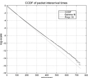
First, we study the OC48 traffic traces, then we apply our methods to the other packet traces captured in the Lawrence Berkeley Laboratory. The series of interarrival times in the OC48 traces are modeled as stochastic series. If the series correspond to a Poisson process, then the interarrival times have exponential distribution. In Fig. 1 we fitted the Gamma distribution to the interarrival times of the OC48 traces cap-tured on April, 24, 2003 (20030424-001000-0-anon.pcap). (The Gamma distribution is more general than the exponential distribution. It reduces to the exponential distribution, if the shape parameter is 1, see Appendix A.) In fact, we fitted both a Gamma distribution by maximum likelihood method and a linear regression to the complementary cumulative distribution function (CCDF). The latter one might be considered some generalized exponential distribution.
Although the estimated parameters (0.945761, 30.3951) suggest that the distribution of the interarrival times is close
3http://www.ita.ee.lbl.gov/html/contrib/LBL-PKT.html
4http://www.tcpdump.org/; http://www.ita.ee.lbl.gov/html/contrib/tcpdpriv.
html; http://www.ita.ee.lbl.gov/html/contrib/sanitize.html
Fig. 1. CCDF and Gamma distribution of the interarrival times.
to the exponential distribution, the Kolmogorov–Smirnov test strongly rejects the hypothesis that the series follows the Gamma distribution. Consequently, the corresponding process cannot be a Poisson process. Therefore we reject the hypothesis that the packet trace follows a Poisson process.
In the search for a distribution that would be suitable for char-acterizing the interarrival times, the family of Lévy processes is our next direction.
The Poisson process is one of the simplest Lévy processes (see, e.g., [29]) with the main assumption that the incre-ments—the differences of consecutive observations, in our case the interarrival times—are independent, homogeneous and exponential. Changing the distribution of the increments we obtain a wide variety of Lévy-stable processes as candidates for modeling the interarrival times [36]. Lévy-stable processes show heavy tail behavior making it impossible to apply them for the measured interarrival times: Fig. 1 depicts that there are very few measurements after 200 micro second. The heavy tail of a distribution also implies that the moments do not exist, so these distributions are not appropriate for modeling purposes. Other members of the family of Lévy processes, the STLFs, have higher order moments. Since they have been successfully applied for finance, biological, and physical phenomena it seems plausible to apply it for traffic analysis as well. Some applications of the STLFs are demonstrated in [11], [18], [22], and [35]. The following formula of the cumulants of STLF pro-vides a means for estimating the parameters by the method of moments, i.e., calculating the empirical values from the traffic traces and compare them with the theoretical values above:
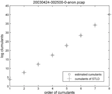
Fig. 2. Comparison of the cumulants and estimated cumulants of the OC48 trace.
TABLE II
ESTIMATEDPARAMETERS OF THEOC48 5-MINUTETRACES INDIRECTION“0”
More precisely, for a given trace we calculate the estimated
cu-mulants , , then we use the least squares
method for finding the estimates , , and (see Appendix D). We carried out these calculations for the OC48 trace cap-tured on April 24, 2003 (20030424-002500-0-anon.pcap). Fig. 2 shows the log of estimated cumulants , and the log of
cu-mulants , , of the STLFs when the
param-eters are estimated, i.e.,
where , , . Since the
fit-ting is good, it implies that this trace is close to the self-similar process because the value of is very small. At the same time the trace is not too far from the exponential distribution consid-ering that the value of is small and is close to 1.
Tables II and III show the estimated parameters of the OC48 5-minute traces.
In general, we can conclude that the distribution of these traces are close to -stable distribution, since the estimations of are very small, hence the process is close to a self-similar
TABLE III
ESTIMATEDPARAMETERS OF THEOC48 5 MINUTETRACES INDIRECTION“1”
process (see Property 1 in Section II-A). It is also clear from the parameters that the traces in direction “1” are closer to the exponential distribution (see Property 2 in Section II-A) than the ones in direction “0”, since the parameter is small and is close to 1 at least in these traces: 05_1, 10_1, 25_1, 45_1, and 50_1. Therefore, the traces in direction “1” are closer to a Poisson process then the traces in direction “0”.
It was pointed out in [15] that the interarrival time distribu-tion includes bursts of back-to-back packets separated by longer times. Similarly to [15] we considered back-to-back packets with less than 6 s for the interarrival time. We ran the previous computations for the traces without back-to-back packets. We found that the values of lambda increased around three times in direction 0 and tenfold in direction 1 relative to the lambda in Tables II and III. As a result, the distribution of the traces signif-icantly deviated from the self-similar distribution. At the same time, since alpha also increased, the heavy-tail property of the distribution was even more emphasized. Similar results can also be found in [15, Fig. 1]; the heavy-tail property of the distribu-tion in [15, Fig. 1.a] is clearly visible above 220 s interarrival times.
V. PACKETLENGTHS
Now, we turn our attention to the investigation of the packet lengths of the traffic traces. We are going to model the packet lengths as increment series of some processes with sta-tionary increments. We fitted both self-similar (non-Gaussian) and “linear” fractal (unifractal) models (see Appendix E) based on higher order cumulants (see Appendix B). The self-similar model is less definite, since the only statistics we use are the cu-mulants of the marginal distribution while the unifractal model is very specific with known distributional properties. The simi-larity in these two models is that the parameters denoted by and are the ones characterizing the long-range dependence of the processes.
For a trace we consider the time series of the packet lengths in some unit time interval, e.g., 100 s. Since the original traces include the packet sizes along with timestamps, the series of packet sizes can be considered as observations in random time making the characterization of the traces difficult, since we do not know the exact distribution of the random time. Rather, we use the sum of the sizes of the packets arriving in
Fig. 3. Self-similar model fitting to the cumulants.
100 s. We choose the 100 s because it is in the order of precision of the packet traces.
We estimate the cumulants according to the formula in Appendix C after estimating the moments, then apply the formula (7), i.e.,
(9) For fix we calculate the left hand side of (9) for different values of aggregation level , then is estimated
taking regression to
and constant 1. Now, if self-similar model is assumed, then
in (9). After is estimated, , the estimate
of the Hurst exponent is simply
For a unifractal model we have .
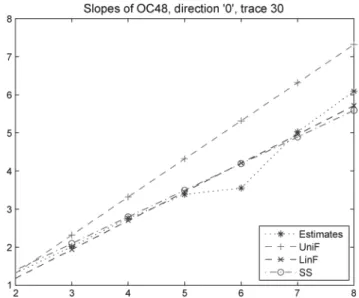
For the sake of the representation, we use a re-weighted least squares method for the estimation of . Additionally, we es-timate some more parameters as well (see (19) in Appendix E). As an example, consider the packets from the OC48 trace 25_0. We plotted the estimated log-cumulants
versus for
in Figs. 3 and 4. The figures show that the log-cumulants of packets from the OC48 trace 25_0 are fitting on some
lines for each fixed . After and are
estimated, the lines are depicted according to the formula .
Both models work well this time, although the parameters and are significantly different. If we assume the linear fractal model, where
, then the estimation of is obtained after linear
regression of , , on . If
the regression parameters are and , then . We
Fig. 4. Unifractal model fitting to the cumulants.
Fig. 5. Fitting lines to the estimated slopes of log-cumulants with different order.
plot these three lines, namely , , and together with the estimated slopes of in Fig. 5. It is natural that the line “LinF” based on linear regression fits best. The problem with the linear regression is that we do not know any result, which describes the probabilistic structure of this type of processes except the challenging definition of dilative stability in [12] (see also in Appendix E). Nevertheless, we keep estimating all three parameters , and for other traces as well.
We continue our analysis with the LBL traces. We obtain for the estimates of the Hurst parameter:
LBL_PKT_4 TCP:
TABLE IV
RESULTS OF THEANALYSES OF THEOC48 TRACES INDIRECTION“0”
TABLE V
RESULTS OF THEANALYSES OF THEOC48 TRACES INDIRECTION“1”
The results of the analyses of the OC48 traces are summarized in Tables IV and V.
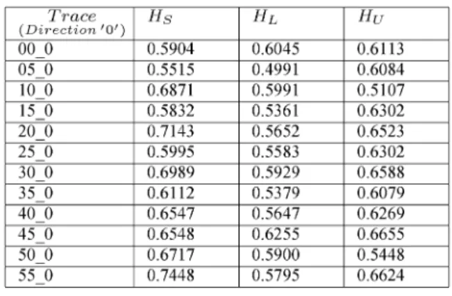
We conclude that all OC48 traces of both directions have long-range dependence parameter less than the middle of the admissible interval [1/2,1). Therefore, the burstiness decreased significantly compared to earlier traces like Belcore trace BC10Oct89 [19] or LBL_PKT_4 TCP and LBL_PKT_5 TCP where the long-range dependence parameter was found to be close to 1.
We can measure the self-similarity by the distance of the self-similar model from the linear fractal model in the following way: Let be the norm of the difference between the esti-mated slopes and slopes from the self-similar modeling and sim-ilarly, let be the norm of the difference between the esti-mated slopes and slopes from the linear fractal modeling, both
for . Consider the ratio , which is
smaller than 1 in general. The ratio is close to 1, if the self-sim-ilar model fits as good as the linear fractal model. Table VI shows that traces of both directions can be modeled by self-sim-ilar model in a reasonably high precision. The exceptions are the traces OC48_0: 10, 20, 40, 55 and OC48_1: 00, 30.
VI. CONCLUSION
In this paper we have considered the problem of modeling high speed-network traces. One of the most interesting ques-tions is the self-similarity nature of these time series. Instead of taking a yes-or-no position we characterized these traces with three parameters of Lévy Flights and positioned a particular
trace somewhere in the space generated by the Poisson and self-similar Lévy processes. We compared the series of the inter-arrival times of the OC48 traces captured by CAIDA in both di-rections. We found that the traces in direction 1 are closer to the Poisson processes than in the other direction. For the time series of packet lengths of the same traces we provided three models: self-similar, unifractal, and linear fractal. The common prop-erty of these models is the long-range dependence. All models fit on the OC48 traces prove the decrease of dependence, and therefore the decrease of burstiness. The common plot of slopes of the log-cumulants of the estimates according to the different models showed the applicability of these models for the traces. Both the self-similar and unifractal models are particular cases of the linear fractal model. The linear fractal model fit for all traces reasonably well and the self-similar model was better than the unifractal model. This happened since the unifractal model was preferable only in the case when the Hurst parameter was close to the upper boundary, which is 1. We also compared the goodness of fit of self-similar model versus linear fractal model for the OC48 traces.
APPENDIX
A. Gamma Distribution
The Gamma pdf is
where and are positive and called shape and scale parameter, respectively. If , then it reduces to the exponential distri-bution.
B. Cumulants
It is well known that there is a one-to-one correspondence between the moments and cumulants. The expected value is the cumulant of first order:
The cumulants of order 2 and 3 are equal to the central moments:
(10) but this is not true for higher order cumulants. One might easily check this for the case of cumulants of order four. Let us denote
the central moment of th order by , then
we have
TABLE VI
GOODNESS OFFIT OFSELF-SIMILARMODELVERSUSLINEARFRACTALMODEL
(see [17, p. 64], [33, p. 10]). If a sample is given, then the estimated expected value, i.e., first order cumulant is the mean , and the estimated th order central moment
Now, the estimated cumulants are given in terms of estimated central moments (see formulae (11) above). For example, the 4th order estimated cumulant is calculated by
C. STLF
Let us recall that the STLF is a Lévy process, i.e., a process with homogeneous and independent increments and . The probability distribution of has characteristic function of the form
where the cumulant function
and , , , is a real number, and
for for
for .
(See [35] for details.)
Without loss of generality, we only consider the case when the shift parameter . Parameters and describe the
skew-ness of the probability distributions, and yields a symmetric distribution. Parameter will be referred to as the
truncation parameter.
In the case of , the cumulant function is given by the formula
(12) and if , the cumulant function
(13) describes a distribution totally concentrated on the positive half-line. The distribution of will be denoted by . The index corresponds to the nontruncated limit when . In this case the distribution of is the classical Lévy’s -stable probability distribution. The scale parameter tunes the time
unit to , hence the distribution of is .
The role of the truncation parameter is obvious in the fol-lowing particular case. For the one-sided dis-tribution with , the cumulant function has the form
(14)
As , the distribution converges to the
-stable distribution . The parameter looks appropriate for measuring the distance from the -stable distri-bution, but it can be noticed that scaling will change the value of as well. More precisely, if distributed as
then the distribution of is , where
. Therefore the distance from the -stable distribution can be measured by the parameter when the value is fixed to 1.
For a fixed , as , the distribution tends to the Gamma distribution . Indeed, for , the
Laplace transform of is
and
by the L’Hospital rule.
D. Estimating the Parameters of
Take the logarithm of
We obtain
(15) Plug the estimated cumulants (see (11) above) into the left side of (15), then we have three unknowns , , and . In order to find the parameter values for the best fitting start with the system of equations when ,3,4, i.e.,
(16)
(17)
(18) The difference of the first two (16), (17) gives
hence
Similarly from the last two (17), (18)
therefore we obtain
We obtain more precise estimations for the parameters, if we use these estimates as initial values and refine the estimates using nonlinear least squares, which minimizes
E. Unifractal Process
The unifractal process has several interesting proper-ties. It is nonlinear and non Gaussian with the same covariance function as FGN. In particular, it has been constructed for de-scribing high speed network traffic, since the traffic is a super-position (aggregation) of several individual traces (see [12]). Moreover, we have the exact expression for the , namely,
(19) where , , are parameters and
The parameters , , of this model are estimated in two steps. First we estimate the left side of (8) for different and use then linear regression on the , weighted according to . The regression coefficient provides the estimate of . The next step is the estimation of , using the expression (19) and when is given. Therefore, we are able to compare the estimated cumulants to the theoretical ones, which are calculated after the parameters , , are estimated.
The stochastic process is called dilative stable, if for all real numbers,
with some positive exponents and , where means the equality of finite-dimensional distributions and denotes the convolution power.
REFERENCES
[1] M. E. Crovella and A. Bestavros, “Self-similarity in World Wide Web traffic: evidence and possible causes,” IEEE/ACM Trans. Networking, vol. 5, no. 6, pp. 835–846, Dec. 1997.
[2] A. Erramilli, O. Narayan, and W. Willinger, “Experimental queueing analysis with long-range dependent packet traffic,” IEEE/ACM Trans.
Networking, vol. 4, no. 2, pp. 209–223, Apr. 1996.
[3] A. Feldmann, A. C. Gilbert, and W. Willinger, “Data networks as cas-cades: Investigating the multifractal nature of the Internet WAN traffic,” in Proc. ACM SIGCOMM, 1998, pp. 42–55.
[4] A. Feldmann, A. C. Gilbert, P. Huang, and W. Willinger, “Dynamics of IP traffic: A study of the role of variability and the impact of control,” in Proc. ACM SIGCOMM, 1999, pp. 301–313.
[5] W.-B. Gong, Y. Liu, V. Misra, and D. Towsley, “Self-similarity and long range dependence on the Internet: A second look at the evidence, origins and implications,” Comput. Netw., vol. 48, no. 3, pp. 377–399, June 2005.
[6] T. Gyires, “Simulation of the harmful consequences of self-similar net-work traffic,” J. Comput. Inf. Syst., pp. 94–111, Summer, 2002. [7] G. He, Y. Gao, J. C. Hou, and K. Park, “A case for exploiting
self-sim-ilarity of network traffic in TCP congestion control,” Comput. Netw., vol. 45, no. 6, pp. 743–766, Aug. 2004.
[8] G. He and J. C. Hou, “On sampling self-similar Internet traffic,”
Comput. Netw., vol. 50, no. 16, pp. 2919–2936, Nov. 2006.
[9] N. Hohn, D. Veitch, and P. Abry, “Does fractal scaling at the IP level depend on TCP flow arrival processes?,” presented at the Internet Mea-surement Workshop (IMW 2002), Marseille, France, Nov. 2002. [10] N. Hohn, D. Veitch, and P. Abry, “Cluster processes: a natural language
for network traffic,” IEEE Trans. Signal Process., vol. 51, no. 8, pp. 2229–2244, Aug. 2003.
[11] P. Hougaard, “Survival models for heterogeneous populations derived from stable distributions,” Biometrika, vol. 73, no. 2, pp. 387–396, 1986.
[12] E. Iglói and G. Terdik, “Superposition of diffusions with linear gener-ator and its multifractal limit process,” ESAIM Probab. Stat., vol. 7, pp. 23–88, 2003, (electronic).
[13] H. Jiang and C. Dovrolis, “Source-level packet bursts: Causes and effects,” presented at the Internet Measurement Conf. (IMC 2003), Miami, FL, Oct. 2003.
[14] H. Jiang and C. Dovrolis, “Why is the Internet traffic bursty in short time scales,” ACM SIGMETRICS Perform. Eval. Rev., vol. 33, no. 1, pp. 241–252, Jun. 2005.
[15] T. Karagiannis, M. Molle, M. Faloutsos, and A. Broido, “A nonsta-tionary Poisson view of Internet traffic,” in Proc. IEEE INFOCOM
2004, Hong Kong, Mar. 2004, vol. 3, pp. 1558–1569.
[16] S. Karlin and H. M. Taylor, A First Course in Stochastic Processes, 2nd ed. New York, London: Academic, 1975.
[17] M. G. Kendall, The Advanced Theory of Statistics. Philadelphia, PA: J. B. Lippincott Co., 1944, vol. I.
[18] I. Koponen, “Analytic approach to the problem of convergence of trun-cated Lévy flights towards the Gaussian stochastic process,” Phys. Rev.
E., vol. 52, pp. 1197–1199, 1995.
[19] W. E. Leland, M. S. Taqqu, W. Willinger, and D. V. Wilson, “On the self-similar nature of Ethernet traffic (extended version),” IEEE/ACM
Trans. Networking, vol. 2, no. 1, pp. 1–15, Feb. 1994.
[20] W. E. Leland, M. S. Taqqu, W. Willinger, and D. V. Wilson, “Statistical analysis and stochastic modeling of self-similar data traffic,” in The
Fundamental Role of Teletraffic in the Evolution of Telecommunica-tions Networks, Proceedings of the 14th International Teletraffic Con-gress (ITC ’94), J. Labetoulle and J. W. Roberts, Eds. Amsterdam: Elsevier Science B.V., 1994, pp. 319–328.
[21] W. E. Leland and D. W. Wilson, “High time-resolution measurement and analysis of LAN traffic: Implications for LAN interconnection,” in
Proc. IEEE INFOCOM’91, Bal Harbour, FL, 1991, pp. 1360–1366.
[22] R. N. Mantegna and H. E. Stanley, “Stochastic processes with ultraslow convergence to a Gaussian: The truncated Lévy flight,” Phys. Rev. Lett., vol. 73, pp. 2946–2949, 1994.
[23] S. Molnár and G. Terdik, “A general fractal model of Internet traffic,” in
Proc. 26th Annu. IEEE Conf. Local Computer Networks (LCN), Tampa,
FL, Nov. 2001, pp. 492–499.
[24] K. Park, M. Kim, and G. Crovella, “On the relationship between file sizes, transport protocols, and self-similar network traffic,” in Proc. 4th
Int. Conf. Network Protocols (ICNP’96), 1996, pp. 171–180.
[25] V. Paxson and S. Floyd, “Wide-area traffic: The failure of Poisson mod-eling,” IEEE/ACM Trans. Networking, vol. 3, no. 3, pp. 226–244, Jun. 1995.
[26] J. Rosinski, “Tempering stable processes,” Stochast. Process. Applicat., vol. 117, pp. 677–707, 2007.
[27] G. Samorodnitski and M. S. Taqqu, Stable Non-Gaussian Random
Pro-cesses. Stochastic Models With Infinite Variance. New York, London: Chapman and Hall, 1994.
[28] S. Sarvotham, R. Riedi, and R. Baraniuk, “Connection-level analysis and modeling of network traffic,” presented at the ACM SIGCOMM In-ternet Measurement Workshop (IMW 2001), San Francisco, CA, Nov. 2001.
[29] K. Sato, Lévy Processes and Infinitely Divisible Distributions. Cam-bridge, U.K.: Cambridge Univ. Press, 1999, vol. 68, Cambridge Studies in Advanced Mathematics, translated from the 1990 Japanese original, revised by the author.
[30] Y. G. Sinai, “Self-similar probability distributions,” Theor. Probab.
Appl., vol. 21, pp. 64–84, 1976.
[31] K. Sriram and W. Whitt, “Characterizing superposition arrival pro-cesses in packet multiplexers for voice and data,” IEEE J. Sel. Areas
Commun., vol. 4, no. 6, pp. 833–846, Sep. 1986.
[32] M. S. Taqqu, V. Teverovsky, and W. Willinger, “Is network traffic self-similar or multifractal?,” Fractals, vol. 5, no. 1, pp. 63–73, 1997. [33] G. Terdik, Bilinear Stochastic Models and Related Problems of
Non-linear Time Series Analysis; A Frequency Domain Approach. New York: Springer Verlag, 1999, vol. 142, Lecture Notes in Statistics. [34] G. Terdik and W. A. Woyczynski, “Rosiñski measures for tempered
stable and related Ornstein-Uhlenbeck processes,” Probab. Math.
Statist., vol. 26, no. 2, pp. 213–243, 2006.
[35] G. Terdik, W. A. Woyczynski, and A. Piryatinska, “Fractional- and integer-order moments, and multiscaling for smoothly truncated Lévy flights,” Phys. Lett. A, vol. 348, pp. 94–109, 2006.
[36] G. Xiaohu, Z. Guangxi, and Z. Yaoting, “On the testing for alpha-stable distributions of network traffic,” Comput. Commun., vol. 27, no. 5, pp. 447–457, Mar. 2004.
[37] C. Shannon, E. Aben, K. Claffy, D. Andersen, and N. Brownlee, The CAIDA OC48 Traces Dataset. Cooperative Association for Internet Data Analysis (CAIDA), Univ. California San Diego Supercomputer Ctr., La Jolla, CA, Jun. 6, 2008 [Online]. Available: http://www.caida. org/data/passive
[38] E. Iglói, “Self-similarity and dilative stability,” Univ. Debrecen, Hun-gary, 2005 [Online]. Available: http://www.inf.unideb.hu/valseg/dol-gozok/igloi/2005dilative_stable.pdf
György Terdik received the Ph.D. degree from the
Kossuth Lajos University, Hungary.
He is a Professor and Head of the Department of Information Technology at the University of Debrecen, Hungary. His research areas include nonlinear, non-Gaussian time series analysis, Lévy processes, and high-speed network modeling.
Dr. Terdik is a member of the editorial board of the quarterly Publicationes Mathematicae Debrecen.
Tibor Gyires (M’97) received the Ph.D. degree from
the Kossuth Lajos University, Hungary.
He is a professor in the School of Information Technology at Illinois State University. His research areas include search algorithms, high-speed net-works, simulation modeling of netnet-works, network capacity planning, and performance prediction. He has established the Internet 2 Research Lab for conducting research in performance evaluation of high-speed networks.