Dynamic rupture processes inferred from laboratory microearthquakes

HAL Id: insu-01469505

https://hal-insu.archives-ouvertes.fr/insu-01469505

Submitted on 16 Feb 2017

HAL is a multi-disciplinary open access

archive for the deposit and dissemination of

sci-entific research documents, whether they are

pub-lished or not. The documents may come from

teaching and research institutions in France or

abroad, or from public or private research centers.

L’archive ouverte pluridisciplinaire HAL, est

destinée au dépôt et à la diffusion de documents

scientifiques de niveau recherche, publiés ou non,

émanant des établissements d’enseignement et de

recherche français ou étrangers, des laboratoires

publics ou privés.

François Passelègue, Alexandre Schubnel, Stefan Nielsen, Harsha Bhat,

Damien Deldicque, Raùl Madariaga

To cite this version:

François Passelègue, Alexandre Schubnel, Stefan Nielsen, Harsha Bhat, Damien Deldicque, et al..

Dy-namic rupture processes inferred from laboratory microearthquakes. Journal of Geophysical Research :

Solid Earth, American Geophysical Union, 2016, 121 (6), pp.4343-4365. �10.1002/2015JB012694�.

�insu-01469505�

Dynamic rupture processes inferred from laboratory

microearthquakes

François. X. Passelègue1_{, Alexandre Schubnel}1_{, Stefan Nielsen}2_{, Harsha S. Bhat}3_,

Damien Deldicque1_{, and Raùl Madariaga}1

1_{Laboratoire de Géologie, CNRS UMR 8538, École Normale Supérieure, Paris, France,}2_{Department of Earth Sciences,}

University of Durham, Durham, UK,3_{Institut de Physique du Globe de Paris, Paris, France}

Abstract

monitoring array recorded particle acceleration during macroscopic stick-slip events allowing us to estimate rupture speed. In addition, we record the stress drop dynamically and we show that the dynamic stress drop measured locally close to the fault plane is almost total in the breakdown zone (for normal stress>75 MPa), while the friction f recovers to values of f> 0.4 within only a few hundred microseconds. Enhanced dynamic weakening is observed to be linked to the melting of asperities which can be well explained by flash heating theory in agreement with our postmortem microstructural analysis. Relationships between initial state of stress, rupture velocities, stress drop, and energy budget suggest that at high normal stress (leading to supershear rupture velocities), the rupture processes are more dissipative. Our observations question the current dichotomy between the fracture energy and the frictional energy in terms of rupture processes. A power law scaling of the fracture energy with final slip is observed over 8 orders of magnitude in slip, from a few microns to tens of meters.

1. Introduction

Earthquake ruptures nucleate and propagate, because faults lose strength with increasing slip and slip rate. If seismology allows us to estimate many of the earthquake source parameters, for instance, static stress drop, fracture energy, particle motion, seismic moment release, and rupture velocity, the accuracy of these measure-ments remains quite uncertain. In the past decade, numerous laboratory experimeasure-ments have been conducted in order to improve our understanding of earthquake mechanics. This approach is particularly evident in the work of (i) Byerlee and Brace [Brace and Byerlee, 1966; Byerlee and Brace, 1968], who first proposed the mech-anism of stick slip as an analogue for earthquakes, then in the work of (ii) Scholz and Johnson [Johnson et al., 1973; Johnson and Scholz, 1976] who investigated source parameters in the laboratory, and finally, in the work of (iii) Ohnaka [Ohnaka, 2003] who first described the complete mechanism of stick slip, from nucleation to dynamic propagation of rupture. More recently, studies on analogous materials highlighted detailed rupture processes at the scale of the rupture tip, using photoelastic material or laser interferometry. These studies revealed the existence of supershear rupture [Rosakis et al., 1999; Xia et al., 2004; Ben-David et al., 2010], the transition from crack to pulse-like rupture [Lykotrafitis et al., 2006], the development of tensile cracks at the rupture tip [Griffith et al., 2009], and the properties of friction during dynamic rupture propagation [Ben-David

and Fineberg, 2011; Svetlizky and Fineberg, 2014; Bayart et al., 2015]. While these works provided an

invalu-able phenomenological framework, these studies were not invalu-able to fully describe the rupture processes under upper crustal stress conditions as they were limited by both technology and pressure conditions.

On the other hand, the advance of high-velocity shear apparatus has allowed the study of the evolution of fault strength at seismic slip rates [Hirose and Shimamoto, 2005; Di Toro et al., 2011], for slips of the order of natural earthquakes. These studies highlighted numerous possible weakening mechanisms to explain coseis-mic weakening during rupture [Brune et al., 1969], including melt lubrication of the fault surface [Tsutsumi and

Shimamoto, 1997; Di Toro et al., 2006; Nielsen et al., 2008], flash heating [Rice, 2006; Goldsby and Tullis, 2011],

thermal pressurization [Wibberley and Shimamoto, 2005; Rice, 2006], thermal pressurization during mineral dehydration [Han et al., 2007; Brantut et al., 2008, 2010], and thixotropic behavior of silica gels [Goldsby and

Tullis, 2002; Di Toro et al., 2004; Rowe and Griffith, 2015]. These experiments are not directly comparable to

RESEARCH ARTICLE

10.1002/2015JB012694

Key Points:

• Dynamic stress change during laboratory earthquakes

• Complete capture of the weakening processes

• Scaling with natural earthquakes

Correspondence to:

F. X. Passelègue,

francois.passelegue@manchester.ac.uk

Citation:

Passelègue, F. X., A. Schubnel, S. Nielsen, H. S. Bhat, D. Deldicque, and R. Madariaga (2016), Dynamic rupture processes inferred from labo-ratory microearthquakes, J. Geophys. Res. Solid Earth, 121, 4343–4365, doi:10.1002/2015JB012694.

Received 26 NOV 2015 Accepted 23 APR 2016

Accepted article online 2 MAY 2016 Published online 11 JUN 2016

©2016. American Geophysical Union. All Rights Reserved.

natural earthquakes because they do not reproduce the propagation of rupture tip but only the variation of local frictional properties with slip and slip rate on the fault. A remarkable observation of the above studies is that the dynamic friction coefficient (f_d) is expected to become extremely low at high slip rate (v_s> 0.1 m/s), and these weakening mechanisms are activated by heat production along the fault interface [Di Toro et al., 2011]. Hence, under crustal stress conditions (i.e., high normal stress), the resulting strength drop, which can be approximated by Δ𝜏 = 𝜎n(fs− fd), is expected to be much larger than current seismological estimates, at least at the scale of seismic asperities. This behavior could play a key role in the rupture processes and in the radiation patterns during large crustal earthquakes, leading to extreme coseismic accelerations and slip velocities.

Stick-slip experiments are good candidates to study the interplay between shear rupture propagation and dynamic weakening mechanisms, because they result in a rapid and sudden release of the accumulated elas-tic strain during interseismic loading, idenelas-tical to that during earthquake rupture [Brace and Byerlee, 1966]. In addition, advances in high-frequency acoustic monitoring allow imaging of rupture processes using acous-tic emissions [Lockner et al., 1992; Lockner, 1993; Schubnel and Guéguen, 2003; Thompson et al., 2005; Schubnel

et al., 2006, 2007; Thompson et al., 2009; Goebel et al., 2012] (AEs), estimation of damage during

deforma-tion processes by measurement of acoustic wave velocities [Schubnel and Guéguen, 2003; Nasseri et al., 2007], and estimation of rupture velocity during stick-slip experiments [Schubnel et al., 2011; Passelègue et al., 2013]. Numerous stick-slip experiments have been conducted measuring dynamic stress changes during rupture propagation in the past [Johnson et al., 1973; Johnson and Scholz, 1976; Lockner et al., 1982; Lockner and Okubo, 1983; Okubo and Dieterich, 1984; Ohnaka, 2003; Beeler et al., 2012]. But until now, most of the experiments conducted in fully confined conditions were only able to monitor the stress at low sampling rates [Lockner

et al., 1992; Lockner, 1993; Thompson et al., 2009; Goebel et al., 2012], and thus were not able to record the

dynamic weakening processes during stick-slip events, which occur within a time window ranging between 10 to 100 μs only, depending on the sample size [Koizumi et al., 2004].

In this study, we investigated the rupture processes during stick-slip events (referred in the following as STE) on Westerly granite under upper crustal stress conditions, at 10 to 100 MPa of confining pressure (Pc). In particular, we measure both the rupture velocity and the stress drop dynamically close to the fault plane and analyze their respective influence on the rupture processes. Finally, we compare our results with previous experimental studies, linear fracture mechanics theory, and seismological observations.

2. Experimental Setup

2.1. The Triaxial Loading Cell

The apparatus used in this study is a triaxial oil medium loading cell (𝜎1>𝜎2=𝜎3) built by Sanchez

Technologies. The confining pressure is directly applied by a volumetric servo pump up to a maximum of 100 MPa. The axial stress is controlled independently by an axial piston controlled by a similar servo pump. The axial stress can reach 680 MPa on 40 mm diameter samples. Both confining and axial pressure are controlled and measured with a resolution of 0.01 MPa. Axial shortening is measured by averaging the values recorded on three capacitive gap sensors located externally. These sensors record both the sample deformation and that of the apparatus. The resolution of these measurements is 0.1 μm. Both pressure and displacement data are recorded at sampling rates ranging between 10 and 1000˜Hz during experiments. More details can be found in Brantut et al. [2011].

2.2. Sample Preparation

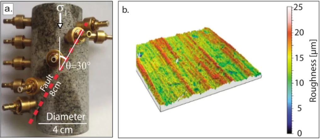
The rock used in these experiments was Westerly granite. The sample is a cylinder of granite with a diameter of 40 mm and a length of 88 mm. The basal areas are ground first with a surface grinder to assure perpen-dicularity to the long axis of the sample. Then, the cylinder is cut at an angle of 30∘ to create a fault interface (Figure 1a). The length of the fault is 80 mm (Figure 1a). Both sides of the fault surface are ground with a sur-face grinder to insure a perfect contact between the two parts of the sample and then roughened with♯240 grit paper to preserve a minimum cohesion along the fault interface in the first steps of loading during triax-ial tests. The average inittriax-ial unconfined roughness of the fault walls was measured using laser interferometry to be approximately ±20 μm (Figure 1b). The sample assemblage is isolated from the confining oil by a neo-prene jacket (125 mm long, 5 mm wall thickness). The jacket is perforated by holes of 7 mm diameter to insert piezoelectric transducers (see section 2.4). The position of each hole is measured with an accuracy of ±1 mm. Transducers are then glued on the rock surface using cyanocrylate adhesive. The sealing between the jacket

Figure 1. Details of the experimental apparatus and of the rock assemblage. (a) The fault system is simulated using

saw-cut Westerly granite sample. The fault plane is inclined at an angle ofΘ = 30∘from𝜎₁. (b) Measurement of the initial roughness of the fault.

and the sensors is provided by two layers of flexible glue (Loctite 9455 Hysol). Finally, teflon shims are gener-ally placed on both sides of the rock specimen in order to reduce the basal friction of the specimen with the piston anvils.

2.3. Strain Gages

External data (collected using the gap sensors) are corrected using the axial deformation of the sample mea-sured using strain gages glued directly on the rock sample. Up to four pairs of strain gages can be used during each experiment. Each pair of strain gages is composed of two resistors (Ω = 120 ohms) measuring, respec-tively, the axial and the radial strain, corresponding to𝜀₁and𝜀₃in the selected frame of reference. Strains are recorded continuously at a sampling rate ranging from 10 to 1000 Hz. Using these measurements, we can esti-mate the elastic constants of the rock during the elastic part of the experiments and correct the shortening measured externally from the rigidity of the apparatus using the following relation:

𝜀FS ax=𝜀 sample ax + Δ𝜎 Eap (1) where𝜀FS

axis the average axial strain measured on gap sensors,𝜀 sample

ax is the axial strain of the sample, Δ𝜎 is

the differential stress and Eapis the rigidity of the apparatus. The rigidity of the apparatus ranges between 25

and 40 GPa depending of the applied load. Using linear elasticity, strain measurements can provide a good estimate of the local static stress change during experiments. Using the measurement of the axial shortening by capacitive gap sensors located externally combined with axial strain gage measurements, we are able to estimate the axial displacement from

D_ax=𝜀sample_ax L = ( 𝜀FS ax− Δ𝜎 Eap ) L (2)

where L is the length of the rock sample. The finite displacement along the fault during stick-slip instabili-ties, also called final displacement, is then estimate using a simple projection assuming Df= Dax∕cos𝜃. All

displacements discussed in the following correspond to displacement along the fault (Df).

In addition to classical strain gages, up to four complete Wheatstone bridge strain gages can be glued directly on the rock sample close to the fault plane (Figure 2a). Each Wheatstone bridge is composed of four resistors (Ω = 350 ohms) measuring together the differential strain𝜀1−𝜀3. The signals are relayed to a high-frequency

strain gage amplifier (Figure 2b) allowing up to 10 MHz sampling rate. The strain gages are calibrated using low-frequency stress and strain measurements during the elastic part prior to each STE (Figure 2c), assuming a constant Young’s modulus (E = 64 GPa) for Westerly granite. Assuming linear elasticity, the measurement at high sampling rate of the differential strain is converted into the dynamic evolution of the differential stress (i.e.,𝜎1−𝜎3) during STE. The assumption of linear elasticity during short time intervals remains robust

because damage is localized during stick-slip instability [Goebel et al., 2014] in comparison with intact speci-mens [Wong, 1982; Hamiel et al., 2009] and do not affect the bulk of the granite at the measurement location. Measurements of stress at high sampling rate were conducted during experiments WGsc16 and WGsc17 only (Table 1).

Figure 2. High-frequency strain measurements. (a) Typical sensors array used to estimate the rupture velocity of

stick-slip instabilities. Yellow sensors are used to invert the rupture velocity. The full bridge strain gage used to record the shear stress change at high sampling rate is located at 5 mm from the fault plane. (b) Picture of the amplifier used to record the stress measurements at 10 MHz. (c) Relation between the signal received using the Wheatstone bridge and the differential stress measured with pressure sensors during the elastic loading. The linear relationship allows one to estimate the stress change during stick-slip instabilities assuming a constant Young’s modulus. (d) Evolution of the stress during stick-slip instability at 130 MPa normal stress. Grey solid line corresponds to raw data. The data have been smoothed using low-pass filter at 200 kHz in order to remove the noise. A strong dynamic stress drop is first observed corresponding to (_𝜏p−𝜏r). The final stress difference corresponds to the static stress drop (𝜏p−𝜏0).

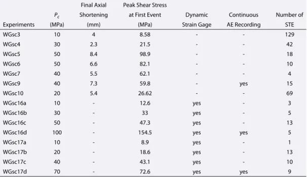
Table 1. List of Stick-Slip Experiments Presented in This Manuscripta

Final Axial Peak Shear Stress

Pc Shortening at First Event Dynamic Continuous Number of

Experiments (MPa) (mm) (MPa) Strain Gage AE Recording STE

WGsc3 10 4 8.58 - - 129 WGsc4 30 2.3 21.5 - - 42 WGsc5 50 8.4 98.9 - - 18 WGsc6 50 6.6 82.1 - - 10 WGsc7 40 5.5 62.1 - - 4 WGsc9 40 7.3 59.8 - yes 15 WGsc10 20 5.4 26.62 - - 69 WGsc16a 10 - 12.6 yes - 3 WGsc16b 30 - 33 yes - 5 WGsc16c 50 - 47.3 yes - 13 WGsc16d 100 - 154.5 yes yes 5 WGsc17a 10 - 8.9 yes - 1 WGsc17b 20 - 18.6 yes - 13 WGsc17c 40 - 43.1 yes - 10 WGsc17d 70 - 72.6 yes yes 9

a_{Some other experiments on serpentinite, peridotite, and intact rocks have also been conducted. The results are not}

Figure 3. The unamplified signals of stick-slip instabilities are

recorded using a second 16-channel digital oscilloscope. In this case, the signals correspond to particle acceleration due to dynamic rupture propagation [Schubnel et al., 2011;

Passelègue et al., 2013].

Raw data presenting the differential stress change during STE observed at 50 MPa confining pressure (middle range of pressure explored in this study) is displayed in Figure 2d. The stress is stable until the passage of the rupture front. Then a strong and abrupt decrease of the stress is observed down to a minimum value. The difference between the peak stress and the minimal value corresponds to the dynamic stress change and can be used to estimate the dynamic shear stress drop by stress rotation, Δ𝜏_dyn = ((𝜎₁−𝜎₃)∕2)sin2𝜃, where 𝜃 is the angle between𝜎1and the normal to the fault

plane (here𝜃 =60∘). After the dynamic stress drop, we observed frame oscillations due to the rapid release of stress. The amplitude of the oscillations decreases with time until the stress reaches a sta-ble value, which corresponds to the final stress [Beeler et al., 2012]. The difference between the initial shear stress and the final stress value is consistent with the static stress drop recorded at low sampling rates. All the data presented below have been smoothed using a low-pass filter at 200 kHz in order to remove high-frequency elastic wave radiation and electrical noise.

2.4. Acoustic Monitoring System

To record acoustic emissions during experiments, we used an array of 16 piezoelectric transducers, each con-sisting of a PZT crystal (PI ceramic Pi255, 5 mm in diameter and 0.5 mm in thickness, 2 MHz central frequency) encapsulated within a brass casing (Figure 2a). Crystals are all polarized the same way so that transducers record waves preferentially polarized perpendicular (P waves) to the sample cylindrical surface. The signal received on each sensor is relayed unamplified through 50 Ohms coaxial cables to a 16-channel digital USB oscilloscope (Figure 3). Unsaturated waveform recordings (Figure 3) were previously shown to correspond to particle accelerations [Schubnel et al., 2011; Passelègue et al., 2013].

The trigger is set such that only the macroscopic dynamic rupture can trigger the record, at 10 MHz sampling rate and up to a volt scale of 80 V.

Amplified signals, at 45 dB, were also recorded to detect acoustic emissions (AE), but are not shown in this study, except in the form of an averaged AE rate. The recording of AEs is triggered when any 3 of the 16 sensors reach a threshold voltage (150 mV) within a 50 μs time window.

3. Mechanical and Acoustic Results

3.1. Low Frequency Mechanical Data

Stick-slip experiments have been conducted at confining pressures ranging from 10 MPa to 100 MPa, i.e. nor-mal stress ranging between 15 and 160 MPa. Cumulative sliding at the end of each experiment was in the range of 2.3 to 8.4 mm (Table 1). Classical results of stick-slip experiments including frictional change, axial shortening, and AE rates are presented in Figures 4 (top) to 4 (bottom) for experiments conducted, respec-tively, at 10 MPa, 30 MPa, and 50 MPa of confining pressure. The friction coefficient is calculated using the strain gages and assuming the Young’s modulus of the Westerly granite. Experiments presented in Figures 4 (top) and 4 (middle) were conducted at a strain rate of 10−5_s−1_{and the experiment presented in Figure 4}

(bottom) was conducted at a strain rate of 10−4_s−1_{. A first effect of the normal stress is observed on the}

aver-age value of the static friction (f_s), prior to instability, which increases from 0.4 to 0.9 between experiments conducted at Pc= 10 and 50 MPa. When friction reaches a critical value, a stress drop is observed. This stress drop is associated with fault displacement (Df). At low normal stress (𝜎n< 40 MPa), the friction drop observed during STEs is almost constant and is between 0.05 and 0.1. At higher normal stress (𝜎n> 40 MPa), the frictional drop increases to value ranging from 0.15 to 0.2 suggesting enhanced weakening along the fault plane. Both displacement and shear stress drops increase with increasing confining pressure. The average value of the static stress drop and of the displacement are respectively 0.5 MPa and 20 μm at𝜎3= 10 MPa and 30 MPa

Figure 4. Evolution of resolved friction coefficient, shear displacement, and acoustic emissions rate during stick-slip

sequences conducted at (top) 10, (middle) 30, and (bottom) 50 MPa of confining pressure. Black, grey, and red solid lines correspond, respectively, to the friction coefficient, axial displacement, and AE rate. At low-confining pressure, only one acoustic emission, corresponding to the stick-slip instability, is recorded during each stick-slip cycle. At higher confining pressure, foreshock activity is observed. The peak friction, the friction drop, and the displacement increase with𝜎₃.

A second effect of the normal stress is observed on the acoustic activity during stick-slip sequences. With the exception of a few events, almost no AE were recorded during the experiments at 10 MPa confining pressure (Figure 4, top) and only the STE are acoustically detected and recorded. Increasing the normal stress leads to an increase of the acoustic activity, in terms of number and amplitude of AE. The peak of AE rate during a stick-slip sequence is generally observed at the onset of instability. Interestingly, the acoustic activity also seems to increase with time, along with cumulative STE displacement (Figures 4, middle and 4, bottom). These AEs are interpreted as foreshocks, which is beyond the scope of this study and is extensively discussed in (F. X. Passelègue et al., Influence of fault strength on precursory processes during laboratory earthquakes, submitted to AGU Monograph Series, 2016).

3.2. Dynamic Stress Drop Measurements

The dynamic evolution of shear stress, i.e., the history of shear stress during sliding recorded close to the fault plane is displayed on Figure 5a for single STEs under a wide range of normal stresses. The shear stress acting on the fault is calculated and normalized using the following expression:

𝜏(t)=

(𝜎₁−𝜎₃)(t)sin2𝜃 2𝜏0

(3) where𝜏0is the shear stress at the onset of the stick-slip instability.

At low normal stress (𝜎n< 30 MPa), the dynamic shear stress drop is moderate and approximately equal to the static stress drop (Δf ≈ 0.1). This observation is in agreement with previous experimental studies conducted without confining pressure [Lockner et al., 1982; Lockner and Okubo, 1983; Okubo and Dieterich, 1984; Ohnaka, 2003; Beeler et al., 2012] and suggests that little weakening is activated during the instability (Figure 5a). Shear stress drop increases with increasing normal stress and can reach, for the highest normal stress inves-tigated (160 MPa), up to 0.8𝜏0, i.e., a major fraction of the initial shear stress. This observation suggests a

dynamic friction coefficient as low as 0.15 (Figure 5a). Note that the final stress drop value is always smaller than the dynamic one, particularly at high normal stress and generally close to the static shear stress drop

Figure 5. Dynamic and static stress drops and microearthquakes scaling law during stick-slip instability. (a) Dynamic

stress change curves recorded during 20 STE. All curves are normalized by the initial shear stress (𝜏₀). Both dynamic and static stress drop increase with the initial state of stress. The weakening timet_ctrends to decrease with stress. Stress oscillations after the dynamic stress drop are probably due to resonance within the frame of the apparatus. (b) Static and dynamic shear stress drops versus peak normal stress at the onset of instability. Small events can also occur at high normal stress, leading to a nonlinear trend. (c.) Static and dynamic shear stress drops versus final displacements. A linear relationship is observed, suggesting that displacement is directly correlated to the amount of stress released during the instability.

measured at low frequency. At low normal stress (𝜎_n< 50 MPa), the relationship between static and dynamic stress drops (Δ𝜏) with normal stress are linear. At high normal stress (𝜎_n> 50 MPa), the relation departs from linearity (Figures 5b). Nevertheless, a linear trend is always observed between the static, the dynamic stress drops, and the final displacement (Figure 5c). These results suggest that the initial state of stress is not always correlated with the magnitude of instabilities (i.e., small events can occur at high normal stress). However, the slip, and thus the moment magnitude of our instabilities, directly scale with both dynamic and static stress drops (Figure 5c). The larger the dynamic stress drop, the larger the final stress released and the larger the seismic displacement.

A second observation is that the characteristic weakening time (tc), i.e. the time required to reach the mini-mum shear stress, is not constant and decreases with normal stress. At low normal stress, tcis between 40 and 70 μs while at high normal stress (𝜎n> 30 MPa), tcremains almost constant with values ranging between 20 and 30 μs (Figure 5a), with some exceptions around 10 μs, apparently not correlated to normal stress.

3.3. Rupture Velocity

Because piezoelectric transducers actually record the passage of the rupture front [Schubnel et al., 2011;

Passelègue et al., 2013], the rupture velocity can be simply estimated using the dominant arrival recorded

on the near-field sensor records (Figure 2a), for each macroscopic stick-slip event (STE). This assumption is expected to be valid given that theory predicts that in the near field, the elastic strain should be dominated by the r−n_{(n = 1∕2; V}

r < CR, 0 < n ≤ 1∕2; CS < Vr < CP) singularity close to the rupture tip. Due to the 3-D experimental geometry, a complex mixed-mode rupture can develop. Under the applied loading conditions, the principal slip direction is parallel to the fault length (main axis of the ellipsoidal fault). As a consequence, a mode II (in-plane) rupture will propagate along the fault length, while a mode III (antiplane) rupture will prop-agate along its width. This implies that the rupture velocity, Vr, along the fault length (mode II) is such that Vr< CRduring a sub-Rayleigh rupture and CS< Vr< CPduring a supershear rupture (CR, CS, and CPbeing the Rayleigh, shear, and compressional elastic wave velocities, respectively). In the Mode III direction, along the fault width, rupture velocity is always Vr< CS. For simplicity we approximate the shape of the rupture front as circular at sub-Rayleigh velocity and as elliptical at supershear velocity, where the ratio of the two axes corre-sponds to the ratio of the velocities in the in-plane direction. For each STE, the first wave arrival recorded on each sensor was manually picked for better accuracy. The location and the rupture velocity are then inverted using a least squares method comparing the experimental arrival times to theoretical arrival times calculated using the approximate rupture front geometry described above. To be more precise, the theoretical arrival times are calculated as a function of (i) the possible rupture velocity Vralong strike, varying from 0.1CRto CP, (ii) the rupture front geometry (circular rupture front up to Vr = CR, elliptical above CS), (iii) the time of initi-ation of the event, and finally (iv) the positions of the sensors relative to the nucleiniti-ation zone of rupture. We assume that the lowest residual time (the average value is 0.7 μs) outputs the best solution for (i) the location of the nucleation zone, (ii) the time of initiation, and (iii) the average rupture velocity along strike. Thereafter the value of the rupture velocity at a given point of the fault can be estimated during supershear event using

V_r(X,Y)= _√ 1 cos2_𝛼 C_S2 + sin2_𝛼 V_II2 (4)

where VIIis the rupture velocity parallel to the slip direction,𝛼 is the angle between the coordinates of the given point (X, Y), and the mode III direction is perpendicular to the slip direction (Figure 6a).

Both sub-Rayleigh and supershear ruptures are observed during our experiments [Schubnel et al., 2011;

Passelègue et al., 2013]. Figure 6b presents a travel time plot of the rupture history, i.e., displays the

acous-tic waveforms recorded by near-field sensors as a function of the distance from the nucleation zone for STE

WGsc17♯32. This recording was obtained during an experiment at 70 MPa confining pressure. The signals are

normalized by the maximum amplitude of each trace. As predicted by theory, the near-field sensors do not record any P wave arrival (CP= 5800 m/s), because of their location close enough to the nodal plane. During this event (STE WGsc17♯32, (Figure 6b)), the inversion suggests a supershear rupture, with an average veloc-ity of 4700 m/s, i.e., faster than the Rayleigh wave speed (CR≈ 3300 m/s). In addition, the dynamic shear stress change curve recorded by the dynamic strain gage is displayed on this plot in red. The initiation time of the stress drop is in good agreement with the first wave arrival recorded on each acoustic sensors, confirming that dynamic strain gages also record the rupture front, as demonstrated by previous experimental studies [Johnson et al., 1973; Johnson and Scholz, 1976; Okubo and Dieterich, 1984; Ohnaka, 2003]. Note, however, that due to the location of the strain gages on the rock sample, the dynamic stress change will mainly be related to mode III rupture (i.e., V_IIIup to C_S).

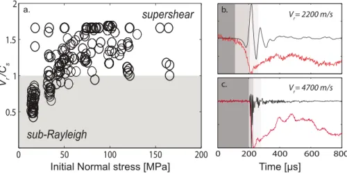
We observe that, during stick-slip experiments in saw-cut Westerly granite, supershear ruptures are system-atically observed when the normal stress exceeds 40 MPa resulting to stress drops between 6 and 40 MPa, comparable to the static stress drops inferred by seismology for crustal earthquakes (Figure 7). The possi-ble implications of this behavior are beyond the scope of this study and have been extensively discussed in

Figure 6. Rupture velocity during stick-slip instability. (a) Schematic of the mixed-mode rupture geometry along the

experimental fault. The rupture is mode II in the in-plane direction (in the strike of the fault) and mode III in the antiplane direction (in the rake of the fault). The rupture front is assumed circular for sub-Rayleigh events and elliptical for supershear events. The rupture velocity at a given point of the fault (Xk, Yk) is a function of mode II and mode III

velocities. (b) Travel time plot of the waveforms recorded on near-fault sensors, displayed as a function of the distance to the nucleation point. The alignment of the first wave arrivals (blue solid line) indicates the average rupture velocity in mode II. In this case, the rupture velocity is faster than the shear wave velocity and the event is supershear. The red solid line corresponds to the dynamic stress change measurement. The first stress drop is in perfect agreement with the first wave arrival recorded on acoustic sensors.

Figures 7b and 7c compare the normalized acoustic waveforms recorded by a sensor located close to the dynamic strain gage and the normalized shear stress change for two STEs, initiated at a similar normal stress and releasing the same dynamic shear stress drop, but presenting two different rupture velocities (i.e., sub-Rayleigh and supershear). The different rupture velocities observed in these two cases can be explained by different initial friction coefficients, respectively, 0.45 for the sub-Rayleigh event and 0.8 for the supershear event. Such a control of the rupture speed by the friction coefficient has been discussed by Ben-David et al. [2010] and Passelègue et al. [2013]. The acoustic waveforms are in good agreement with the stress changes in term of both propagation time and amplitude. Note that in both cases, the strongest particle acceleration is observed when the slope of the shear stress curve (weakening rate term𝛾 (MPa/s)) is maximum. In addition, for the same value of dynamic stress released, the weakening time tcis equal to 83 μs for the sub-Rayleigh

Figure 7. Relationship between the initial state of stress and the rupture velocity. (a) Average rupture velocity as a

function of normal stress acting on the fault plane. (b) Comparison between stress change and particle acceleration recorded by piezoelectric sensors located close to the dynamic strain gage during a sub-Rayleigh event. (c) Same as Figure 7b during a supershear event. In both cases (Figures 7b and 7c), the particle acceleration is in agreement with the stress change and the peak of acceleration is observed when the slope of the stress curve (i.e., the weakening rate_𝛾) is maximum. As expected, the acoustic signal recorded during the supershear event (Figure 7c) presents higher frequency content than during the sub-Rayleigh event (Figure 7b).

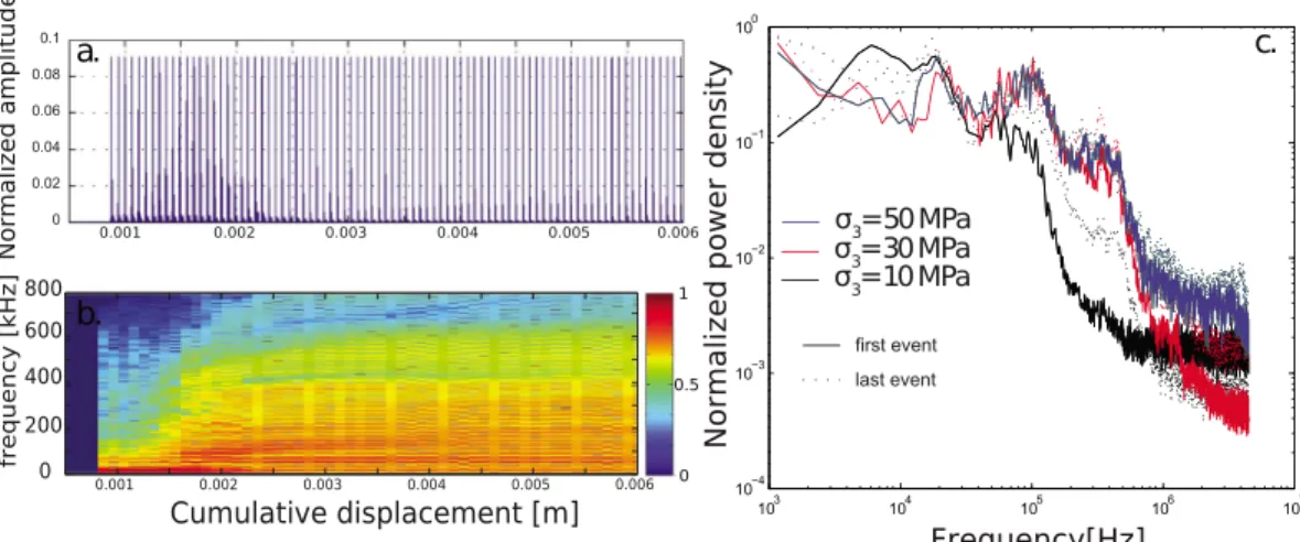
Figure 8. High-frequency radiation during stick-slip motion. (a) Continuous normalized waveform corresponding to all

STE recorded during experiment WGsc3. (b) Spectrogram of frequency content of a single stick-slip event as a function of the cumulative displacement along the experimental fault at 10 MPa confining pressure. The color bar corresponds to the normalized power density also presented in Figure 8c (blue to red from 10−4_{to 10}0_{. (c) Comparison between the}

spectrum of six STE at, respectively, 10, 50, and 100 MPa of confining pressure (first and last events in each condition).

events (Figure 7b) against 12 μs for the supershear event (Figure 7c). These results suggest that the weakening time could be controlled by (i) the rupture velocity and (ii) the absolute value of dynamic stress drop.

3.4. High-Frequency Radiation During Stick-Slip Motion

The evolution of the high-frequency spectrum content of each event, recorded during a single experiment (WGsc3) at Pc= 10 MPa is shown in the form of a spectrogram, as a function of cumulative displacement on Figure 8a. For each event, the waveforms of all the available transducers were normalized in amplitude and then stacked to remove amplitude and to smooth directivity effects. At the beginning of the experiment, no high-frequency radiation is observed (black solid line in Figure 8b). After a cumulative displacement of 1.5 mm, however, high-frequency radiation is recorded within the band 200–400 kHz, and up to 600 KHz after 3.5 mm of displacement.

The spectra of the complete unamplified waveforms recorded during six STEs at 10, 50, and 100 MPa con-fining pressure (first and last events in each pressure conditions) are displayed in Figure 8b. Again, for each event, the waveforms of all the available transducers were normalized in amplitude and then stacked. A dif-ference is observed between STEs recorded at 10 MPa and higher confining pressures, where a strong peak is observed around 100 KHz (Figure 8b). Following a previous study [Passelègue et al., 2013], a transition between sub-Rayleigh and supershear rupture was observed between 10 and 30 MPa of confining pressure during these experiments. This peak seems to correspond to the passage of the shear Mach cone, which present com-patible characteristic [Passelègue et al., 2013]. The second observation is the appearance of a high-frequency peak around 250 kHz. This peak is absent in the spectrum of the waveforms recorded during the first STE of the experiment conducted at 10 MPa confining pressure. This peak is observed in all other spectra. Thus, both increasing normal stress acting on the fault plane and cumulative displacement along the fault pro-mote this radiation. This high-frequency radiation is probably due to the evolution of the fault surface after each dynamic event, in particular, due to fault gouge production and damage-related radiations [Ben-Zion

and Ampuero, 2009; Castro and Ben-Zion, 2013], which could locally perturb the rupture front and produce its

own high-frequency radiation.

4. Microstructural Analysis

Postmortem fault surfaces were analyzed using scanning electron microscopy (SEM). After experiments con-ducted at low normal stress (𝜎_n < 50 MPa), the fault surfaces present striations (Figure 9a) and gouge generated due to the repetition of STEs and associated cumulative displacement. The gouge particles which remained on the fault surface are small, with their size ranging from 100 nm to 10 μm (Figure 9b). This is in good agreement with the general smooth aspect of the fault surface (Figure 9a). On the other hand,

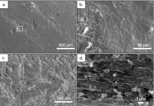
Figure 9. Microtextures of the fault surface after stick-slip experiments under scanning electron microscopy. (a) Striation

and gouge particles after an experiment conducted at low normal stress (P_c= 30MPa,𝜎_n≈50 MPa). (b) Enlarged view of Figure 9a showing dramatic reduction of the grain size due to comminution during instabilities. (c) Amorphous asperities observed after experiment conducted at higher normal stress (Pc= 70MPa,𝜎n≈120 MPa). The size of

asperities is not constant and ranges from 10 to 100μm. (d) Enlarged view of Figure 9c showing evidence of melting at asperities during stick-slip instabilities. Even very small particles, sizes between 0.5 to 2μm, are melted.

gouge particles collected using an ultrasonic bath method immediately after the experiments, and measured using laser granulometry in suspension, present larger sizes between 70 μm and 140 μm. We hypothesize that these larger particles result from the fracture of asperities during the last event, while the small parti-cles which remain attached to the surface even after the ultrasound bath, may have been generated by grain comminution due to cumulative displacement.

At higher normal stress (𝜎n> 50 MPa), the amount of gouge produced is larger while the average particle size is smaller, generally between 1 to 70 μm. In addition, a large portion of the fault plane is covered by smooth and stringy surfaces or asperities (Figure 9c) ranging from 80 to 300 μm in length. An enlarged view of the central part of Figure 9c is presented in Figure 9d. At this scale, we can observe that these smooth and stringy surfaces present stretched microstructures suggesting either high strain plastic deformation or melting of the asperity. The same kind of microstructures have been reported after high-velocity friction experiments on crustal rocks [Hirose and Shimamoto, 2005; Nielsen et al., 2010a] and during stick-slip experiments at higher normal stress [Koizumi et al., 2004; Lockner et al., 2010]. The hypothesis of the partial melting of the fault surface is supported by XRD analyses conducted on fault gouge after an experiment conducted at P_c= 50 MPa, where the characteristic peaks of biotite and feldspar have vanished (Figure 10).

To investigate the internal structure of these patches, a focused ion beam (FIB) section was extracted from the asperity presented in Figure 11a (Pc= 70 MPa). The FIB section was cut perpendicularly to the slipping zone (Figure 11a). SEM and TEM (transmission electron microscopy) micrographs of the FIB section, respectively, displayed in Figures 11b and 11c, reveal a strong deformation gradient. Six micrometers away from the sliding surface, minerals appear fractured and damaged. Approaching the sliding surface, however, a dramatic grain size reduction is observed, suggesting an extreme level of fracturing and comminution (Figures 11b–11d). The latter can be interpreted as thermal cracking, damage due to the stress concentration close to the prop-agating rupture tip, transient high strain rate associated to the shock wave of the supershear rupture, or a combination of all of the above. Finally, right below the fault surface, within a layer of approximately 1 μm thickness (Figure 11c), grains can no longer be observed. Instead, some vesicles of diameter smaller than 100 nm are present.

Figure 10. Comparison between XRD diffractions conducted on intact Westerly granite (black solid line) and fault

gouge resulting from experiments conducted atP_c= 50MPa. The disappearance of the characteristic peaks for the biotite and the feldspar after rupture is observed.

To investigate the evolution of the crystalline state within and close to the slipping zone, electron diffraction patterns were acquired (Figures 11d and 11e). Inside the grains, electron diffraction patterns display well orga-nized diffraction spots (Figure 11f ), which demonstrates that the grains are well crystallized. The diffraction patterns conducted within the thin layer located closest to the slipping zone reveals broad and faint diffu-sion rings and no diffraction spots (Figure 11g). This proves that the layer is composed of amorphous material which demonstrates the occurrence of melting of the fault surface asperities after small localized dynamic slip (from 60 to 250 μm) of extremely short duration (≈15 μs) at elevated normal stress conditions.

5. Interpretation and Discussion

During natural earthquakes, the seismic slip scales with the rupture area, leading to values of stress drop independent of the earthquake size. The results presented in the following differs from natural earthquakes because of the finite size of the fault. The only way to increase the magnitude of the stick-slip events is to increase the elastic strain stored in the medium, i.e., the rock sample and the apparatus. While the slip of each event is mainly controlled by the stiffness of the apparatus, the results in the following are comparable to the rupture of seismic asperities along natural faults which are commonly surrounded by weak or so-called slip-strengthening area.

5.1. Static Versus Dynamic Shear Stress Drop

The relationship between normal stress and dynamic shear stress drops inferred under a wide range of normal stress are presented in Figure 12, along with similar results obtained by previous studies [Johnson et al., 1973;

Okubo and Dieterich, 1984; Lockner et al., 1982; Lockner and Okubo, 1983; Ohnaka, 2003; Beeler et al., 2012]. As

previously stated, the dynamic stress drop increases with increasing normal stress. Solid lines presenting con-stant values of friction drop (assuming Δ𝜏 = (fs− fd)𝜎n) are given for comparison with experimental ones. Results coming from biaxial experiments conducted at low normal stress (𝜎n< 20 MPa) reveal a small fric-tion drop during instabilities with values of Δf (i.e., (fs − fd)) generally between 0.05 and 0.15 [Okubo and Dieterich, 1984; Lockner et al., 1982; Lockner and Okubo, 1983; Ohnaka, 2003; Beeler et al., 2012]. Extrapolating

these results to crustal stresses, using a stress gradient of 27 MPa/km, would result in dynamic stress drops ranging between 16 and 32.5 MPa at 10 and 20 km depth, respectively, which is consistent with seismological observations [Kanamori and Brodsky, 2004].

Making the reasonable assumption that the confining pressure (𝜎₃) remains constant during our experiments, the dynamic frictional drop can be estimated following

f_(t)= ((𝜎1−𝜎3)(t) sin 2𝜃)

((𝜎₁−𝜎₃)(t)(cos 2𝜃 + 1) + 2𝜎₃) (5)

When conducted at low normal stress (𝜎n< 25 MPa), static and dynamic stress drop measurements are similar and suggest a friction drop ranging from 0.1 to 0.3, which is similar to observations performed during biaxial experiments.

The difference between static stress and dynamic stress drops increases with normal stress. Indeed, while the static stress drop seems to be limited to a friction drop of 0.25, the dynamic friction drop at high

Figure 11. FIB section cutting and TEM observations. (a) Picture of the studied asperity. The white line corresponds to

the FIB section. (b) SEM micrograph of the FIB section revealing a strong gradient of the deformation. At 6μm from the sliding surface, the minerals are generally intact and present few cracks. However, approaching the sliding surface, a dramatic grain size reduction is observed suggesting high level of fracturing. An irregular layer of amorphous material is observed below the sliding surface. (c) Large TEM micrograph of the FIB section. Enlarged views of (d) highly fractured grains and (e) amorphous layer. (f ) Electron diffraction patterns revealing well-organized diffraction spots in the highly fractured grains. (g) Diffraction patterns conducted on the superficial layer reveal broad and faint diffusion rings without any diffraction spots.

normal stress (𝜎n> 100 MPa) can be as high as 0.6, suggesting a low dynamic friction coefficient (Figure 12). Such low dynamic friction coefficient is consistent with steady state friction coefficients (fss) observed during

high-velocity friction experiments (Vs> 1 m/s) on crustal rocks [HiroseandShimamoto, 2005; DiToroetal., 2006, 2011]. It can generally be explained by the activation of thermal weakening mechanisms, frictional melting in our case, as supported by our microstructural analysis. Extrapolating to crustal stresses conditions using a similar stress gradient (i.e., 27 MPa/km) would result in dynamic stress drops 1 order of magnitude larger, i.e., ranging between 160 and 320 MPa at 10 and 20 km, respectively. This suggests that, at the scale of seismic asperities, the dynamic stress drop could be much larger (1 order of magnitude) than current seismological estimates of the static stress drop, as also suggested by previous experimental studies [Koizumi et al., 2004] and by high-velocity friction experiments [Tsutsumi and Shimamoto, 1997; Di Toro et al., 2011]. If true, these abrupt variations of stress drop along the fault would certainly contribute to high-frequency radiation.

5.2. Frictional Behavior

The transition to stick-slip instability has been extensively discussed both theoretically and experimentally. Stick-slip motion on faults is generated because faults lose strength with increasing slip and/or slip rate. A widely used frictional law describing this behavior is the rate- and state-dependent law, in which the friction coefficient depends both on the slip rate and on a state variable [Dieterich, 1979; Ruina, 1983]. An alterna-tive extensively used frictional law is the slip-weakening law which describes the evolution of the friction coefficient based solely on the amount of slip [Ida, 1972; Palmer and Rice, 1973; Campillo and Ionescu, 1997].

Figure 12. Comparison of pressure dependence (𝜎_n) of dynamic stress drop with results from previous studies conducted using biaxial apparatus at low normal stress [Okubo and Dieterich, 1984; Lockner et al., 1982; Lockner and

Okubo, 1983; Ohnaka, 2003; Beeler et al., 2012]. The black solid lines correspond to the estimation of the stress drop as a

function of the normal stress followingΔ𝜏 = 𝜎n(fs− fd)where(fs− fd) = Δf. Each line corresponds to different values of

Δf. Squares correspond to dynamic stress drop, and circles correspond to static stress drop. Increasing normal stress acting on the fault plane promote the increase of the friction drop during the instability.

Dynamic friction decreases linearly with displacement, down to a minimum value of approximately 0.15 (Figure 13). This minimum value is controlled by both the slip rate and the Stefan number defined as the ratio of latent heat of fusion to the heat required to raise the temperature from ambient, including heat diffusion effects [Rempel and Weaver, 2008; Nielsen et al., 2008, 2010b]. In other words, if the slip rate (heat source) is large enough so that the heat produced can not be diffused away of the slipping surface anymore, the surface will eventually melt and, consequently, the friction will drop abruptly.

Our observations suggest that the elastic strain accumulated during the interseismic period might in fact con-trol both the local slip rate and the final amount of slip. Experimental results suggest that the frictional drop is controlled solely by slip rate, or the power density (𝜏V_s), at both subseismic and seismic sliding velocities [Dieterich, 1979; Ruina, 1983; Goldsby and Tullis, 2011; Di Toro et al., 2011], which is in qualitative agreement with

Figure 13. Relationships between the stress/friction drop and the final displacement during stick-slip events. Empty

squares and circles correspond, respectively, to dynamic and static stress drops. Full black squares and circles correspond, respectively, to dynamic and static friction drops. While static and dynamic stress drops increase linearly with the amount of slip, dynamic and static friction drops increase linearly until friction drops reach a steady state represented by the shaded area.

Figure 14. Fracture mechanism parameters inferred from high-frequency stress measurements. (a) Comparison of

pressure dependence of critical slip distance. Data are plotted using semilogarithmic scale, revealing thatD_cevolves like a power law as a function of the normal stress. Color bar refers to sliding velocity estimated followingVs= Dc∕tw.

(b) Experimental evidence of the increase ofVswith the rupture velocityVr. However, whileVsincreases withVr, the

range of the sliding velocity is mainly controlled by the dynamic stress drop.

our observations. Our combined dynamic fracture/friction experiments also suggest that the larger the accu-mulated elastic strain, the larger the possible slip rate, the faster the thermal weakening, and consequently a larger final amount of slip. It is important to note that the relation between slip and stress drop remains linear as expected by slip weakening friction law [Ida, 1972; Palmer and Rice, 1973; Campillo and Ionescu, 1997] or by a spring-slider model [Johnson and Scholz, 1976; Shimamoto et al., 1980].

5.3. Critical Slip-Weakening Distance

While we have a direct measurement of the dynamic stress drop Δ𝜏_dynand the rupture velocity V_r(X, Y), we are not yet able to measure the displacement at high sampling rate during stick-slip instabilities, which is an important parameter in the estimation of the critical slip distance (D_c) of the fracture energy (E_g) and of the sliding velocity (Vs). However, assuming a constant rupture velocity and a purely slip-weakening behavior, the critical slip distance Dccan be estimated using [Ida, 1972; Palmer and Rice, 1973; Rice, 1979]

Dc=

16(1 −𝜈) 9𝜋

Vrtc𝜎n(fs− fd)

𝜇 (6)

where𝜇 is the shear modulus of granite (estimated using strain measurements 𝜇 = 34 GPa). Although our measurement of the stress change are not performed directly on the fault plane, the values of Dcobtained using equation (6) can be considered as a good estimate [Svetlizky and Fineberg, 2014], because the weaken-ing time increases with the distance to the fault plane while the strength drop decreases. Usweaken-ing this simple relation, Dcis consistently found smaller than the final displacement. Following previous experimental stud-ies, Dcis supposed to decrease with the amount of shear strain accumulated in the fault core [Marone and Kilgore, 1993], and with heat production during faulting [Niemeijer et al., 2011; Di Toro et al., 2011]. Our

obser-vation is that contrary to previous experimental predictions, D_cincreases both with normal stress and with the dynamic shear stress drop (Figure 14a). At the scale of our experiments, D_cdepends on the final fault displace-ment and thus both on seismic modisplace-ment and normal stress. These results are in qualitative agreedisplace-ment with the scaling of [Ohnaka, 2003]. They strongly suggest that D_cis a thermal parameter, as proposed by recent HVF friction studies [Nielsen et al., 2008; Niemeijer et al., 2011]. Qualitatively, the scale dependence arises from the fact that the larger the stress drop, the faster the rupture velocity, the faster the weakening, the longer

D_c, and thus longer final slip. This is also consistent with the dynamic fracture propagation theory [Ida, 1972;

Palmer and Rice, 1973; Rice, 1979].

5.4. Average Slip Velocity

To estimate the sliding velocity, we use the previous results and assume that the frictional behavior of the fault is purely slip weakening. The critical distance (Dc) can be used to give an average value of the sliding velocity following Vs = Dc∕tw, where twis the weakening time recorded on the dynamic stress change curve (Figures 5a, 7b, and 7c). The relationships between the rupture velocity Vr, the dynamic stress drop Δ𝜏dyn, and

Vsare presented in Figure 14b. In agreement with previous work [Latour et al., 2013; Svetlizky and Fineberg, 2014], we also observe that Vsincreases with increasing rupture velocity. However, our experiments demon-strate that Vsis mainly controlled by the dynamic stress drop (Figure 14b). For a given rupture velocity, the slip velocity can increase by 1 order magnitude due to the increase of Δ𝜏dyn. In our experiments, the dynamic

Table 2. Physical Parameters of Westerly Granite

Parameter Symbol Value Unity

Density 𝜌 2650 kg m−3

Young’s modulus E 64 GPa

Poisson coefficient 𝜈 0.2

-Heat capacity C_p 900 J kg K−1

Weakening temperature T_w 900 ∘C

Initial temperature T_i 25 ∘C

Thermal diffusivity 𝛼 1.25×10−6 _m−2_s−1

stress drop increases with increasing normal stress. Indeed, an increase in normal stress induces an increase of the elastic strain energy stored in the medium (sample + apparatus) so that the larger the stress, the larger the energy release rate at rupture tip and the larger the sliding velocity.

5.5. Heat Production on the Fault

Extreme weakening observed at high normal stress (Figure 13) may be due to the activation of phenomena like melt lubrication or flash heating [Hirose and Shimamoto, 2005; Di Toro et al., 2006; Rice, 2006; Goldsby and

Tullis, 2011]. The parameters defined in the following can be found in Table 2.

The rise of temperature (ΔT) in the slipping zone can be estimated for each STE, assuming a linear decay of the stress as a function of displacement. Once the slip reaches the slip weakening distance D_c, ΔT is equal to

ΔT = 𝜏eVs 𝜌Cp √ Dc 𝜋𝜅Vs (7) where𝜏eis the average stress during the weakening defined as

𝜏e=𝜏r+ 1

2(𝜏p−𝜏r) (8)

and where𝜌 is the rock density (2650 kg m−3_{), C}

pis the heat capacity (900 J kg−1K−1),𝜅 is the thermal diffusivity (1.25 × 10−6_m2_s−1_).

In our experiments, the dynamic friction coefficient continuously decreases with the power density𝜙 (𝜙 =

𝜏eVs) (Figure 15a). The comparison with velocity friction experiments (data from Di Toro et al. [2011]) high-lights that for an equivalent weakening (same value of f_d), the power density required is 2 orders of magnitude higher in our experiments (for f_d = 0.15, Φ_STE= 300 MW and Φ_HVF ≈ 5 MW). However, if we now compute the total heat𝜏_rD_c, the energy required to create an equivalent weakening is 3 orders of magnitude smaller in our experiments (for f_d= 0.15, E_H(STE)= 10 kJ and E_H(HVF) ≈10 MJ). This is explained by the small amount of slip- and short-weakening time during STE in comparison with HVF experiments (Figure 15b). In addition, these discrepancies might partly arise because (1) we use peak sliding velocity and Dcas calculated above to estimate both the power density and the heat, and (2) we assume a linear decay of shear stress and friction with slip. Yet the shift of 2–3 orders of magnitude in power density and heat between HVF experiments and our experiments suggest that asperities, which hold the major portion of shear stress before the instability, probably represent only a small portion of the fault surface which is superheated for a very short time during sliding, producing a transient low viscosity melt.

Our microstructural analyses undoubtedly reveal the presence of a melt layer produced at asperities. Neglecting heat diffusion and considering that all the mechanical work is converted into heat in our experi-ments, the thickness of the melt layer (w) produced can be estimated following (modified from Sibson [1975] and Di Toro et al. [2006]

w = 𝛾 ∗ tw∗ Dc

[L + C_p(T_w− T_i)]𝜌 (9)

where L (2.2 × 105_{J kg}−1_{) is the latent heat of fusion of Westerly granite, T}

ithe initial fault surface tempera-ture, and𝛾 is the average weakening rate during stress drop. Our calculation shows that the dynamic friction is a function of the melt produced during the seismic instability. For the lowest value of dynamic friction coef-ficient, the heat produced is able to melt a layer of a thickness ranging between 1 and 5 μm thick (Figure 15c).

Figure 15. Evolution of the dynamic friction as a function of the heat production. Figures 15a and 15b present the

comparison between our experimental data (circles) and high-velocity friction data (cross) coming from Di Toro et al. [2011]. (a) Evolution of the dynamic friction coefficient,fd, as a function of the power density. (b) Evolution offdas a

function of the heat energy produced during the seismic slip. (c) Estimation of the thickness of the melt layer produced during each stick-slip event assuming an adiabatic system.

This range of values is in agreement with our microstructural analysis (Figure 11b). In addition, we observe that f_dstarts to decrease dramatically when the thickness of the melt layer becomes larger than 0.1 μm. While these range of values for the melt layer are not comparable with microstructural observations after HVF, these results seem in agreement with flash heating theory [Rice, 2006; Rempel and Weaver, 2008; Goldsby and Tullis, 2011], where only a fraction of melting is required to observe strong weakening [Goldsby and Tullis, 2011;

Brown and Fialko, 2012].

5.6. Flash Heating as the Potential Weakening Mechanism

The dramatic weakening induced by flash heating is explained by the melting of small asperities along the fault surfaces when the sliding velocity becomes larger than a weakening velocity (Vw), corresponding to the velocity required to induce the melting of asperities during their contact lifetimes. V_wis a function of the thermal properties of the rock, the size of the asperities and the contact shear strength at the asperities. The contact shear strength is generally larger than the macroscopic shear stress applied on the fault because the real area of contact is much smaller than the nominal area resulting in high contact stresses at asperities. While in the general case flash heating is independent of normal stress, our present case is different because the stress acting on the fault is an important parameter which controls the stress drop and the sliding velocity reached during the instability.

Following microstructural analysis (Figure 9c, 9d, and 10a), the size of asperities is not constant along the fault surface and ranges from 1 μm to 200 μm. Because the contact shear strength is also a function of the size of the asperities, we replaced in flash heating theory [Rice, 2006; Rempel and Weaver, 2008], the term𝜏2

cD𝛼, where 𝜏cis the contact shear strength on asperities and D𝛼the average size of asperities, by a critical stress intensity parameter KII

𝛼which can be expressed as

Figure 16. Flash heating mechanism during stick-slip instabilities. (a) Evolution of the dynamic friction drop as a

function of the initial state of stress along the fault planeKII

𝛼. The higher the initial state of stress, the larger the dynamic

friction drop. The black solid line corresponds to the evolution of the critical weakening velocity leading to flash weakening as a function ofKII

𝛼. (b) Evolution of the dynamic friction coefficient with the peak of sliding velocity. When V_s< V_w,f_dis generally≈0.5 in agreement with friction experiments conducted at low normal stress. WhenV_s> V_wand

KII

𝛼∕KcII> 1, the decrease offdwithVsis in perfect agreement with flash heating theory [Rempel and Weaver, 2008]. where Lf is the size of the fault. This term can be calculated for each event (Figure 16a) and, based on microstructural analysis (SEM), we can define an average critical value for KII

c, which corresponds to the critical value of KII

𝛼above which melt patches are observed on postmortem fault surfaces. This critical value is equal to KII

c ≈7.5 MPa √

m(Figure 16a). This range of value is similar to those found in previous studies comparing experimental data with flash heating theory [Kohli et al., 2011; Goldsby and Tullis, 2011; Passelègue et al., 2014]. The weakening velocity leading to flash weakening can then be estimated for different values of KII

𝛼, following (modified from Rempel and Weaver [2008])

V_w= (𝜌Cp) 2_(T w− Ti)2𝜋𝜅 (KII 𝛼)2 (11) Using this parameter, we now estimate the friction drop due to flash heating phenomena as a function of the sliding velocity. In our case, the melt layer can be considered as smaller than the characteristic heat diffusion length 4√𝜅𝜃, where 𝜃 = D_𝛼Vs. The evolution of the friction coefficient as a function of the sliding velocity can then be estimated using [Rempel and Weaver, 2008]

f_(Vs)= f_sVw Vs ⎡ ⎢ ⎢ ⎢ ⎣ 1 + 2S ⎛ ⎜ ⎜ ⎜ ⎝ √ V_s Vw − 1 + (1 − S) ln(1 + √_V s Vw − 1 S ) ⎞ ⎟ ⎟ ⎟ ⎠ ⎤ ⎥ ⎥ ⎥ ⎦ (12)

where S is the Stefan number defined by S = L∕[C_p(T_w− T_i)]. At high normal stress, when KII

c> K𝛼II, theoretical prediction is in perfect agreement with our experimental data (Figure 16b). These results suggest that at high normal stress flash heating could promote melting at asperities, at least at the scale of our experiments and a dramatic reduction of the dynamic friction coefficient. Increasing the normal stress acting on the fault leads to (i) an increase of the shear strain accumulated during the interseimic loading, (ii) an increase of the dynamic stress drop, and hence (iii) an increase in the sliding velocity [Brune, 1970]. This large increase of the sliding velocity with normal stress allows the activation of melt lubrication, which promotes complete release of the stress during laboratory earthquakes generated under high stress conditions. Interestingly, at the other end of the spectrum, when the stress acting on the asperities is smaller than KII

𝛼, the observed friction drop is larger than expected and may be due to the production of gouge along the fault.

6. Energy Budget of Laboratory Quakes

6.1. Energy Budget and Radiation Efficiency

Using the previous estimates of Dcand our direct measurements of dynamic stress drop, static stress drop, and final displacement, the energy budget of stick-slip instabilities can be estimated under some simple assump-tions (Figure 17). This energy budget consists of the calculation of the total fracture energy E_g(corresponding to both the weakening and healing steps (Figure 17). E_gis estimated following

Eg=

Dc(𝜏p−𝜏r)

Figure 17. Schematic of the energy budget during

laboratory earthquakes.E_gcorresponds to the total amount of fracture energy during the instability.E_r

corresponds to the radiated energy andE_hcorresponds to the frictional energy. In our experiments,_𝜏0is almost equal to𝜏_pbecause we forced the system to reach the instability.Dcorresponds to the final value of the displacement thereforeD − D_crepresents the displacement expected during the stress recovery.

where𝜏_pis the initial stress at the onset of instability and𝜏_r is the residual stress during the dynamic rup-ture. As in previous experimental studies [Wong, 1982;

Ohnaka, 2003], the healing part of the curves can not

be used because of frame oscillations of the apparatus. The frictional energy Ehis estimated following Eh=𝜏rD and the radiated energy Eris calculated following

Er= ( 1

2(𝜏p−𝜏f) + (𝜏f−𝜏r)) ∗ D − Eg (14) where 𝜏_f is the final stress after the instability. The evolution of E_g, E_h, and E_r with the final displace-ment and as a function of the sliding velocity is presented in (Figure 18a). E_g, E_h, and E_r all increase with seismic moment (i.e., the final displacement). However, for the same initial fault surface, the parti-tioning between these energies strongly depends on the final displacement.

These observations on the energy partitioning are in qualitative agreement with our estimations of D_c. Indeed, at low normal stress, D_cis generally estimated to be around 1 to 10 μm and scales with the rough-ness of the fault, as proposed by previous experimental studies [Marone, 1998; Ohnaka, 2003; Svetlizky and Fineberg, 2014]. However, at higher normal stress, because

D_cbecomes a thermal parameter which continuously increases with normal stress, probably both because

Figure 18. Energy budget of stick-slip instabilities. (a) Evolution ofE_g,E_h, andE_ras a function of the displacement, i.e., the magnitude of the laboratory quakes. Circles, squares, and stars correspond, respectively, toE_g,E_r, andE_h. Color bar corresponds to the peak of sliding velocity of each stick-slip instability. (b) Evolution of the radiation efficiency as a function of the final displacement. Color bar corresponds to the dynamic friction drop of each instability.

Figure 19. Comparison of seismic slip dependence of fracture energy (G) with previous experimental results on saw-cut samples [Ohnaka, 2003] and on intact rocks [Wong, 1982; Ohnaka, 2003] and with seismological observations

[Venkataraman and Kanamori, 2004; Abercrombie and Rice, 2005; Tinti et al., 2005, 2009]. For our study, the seismic slip of laboratory experiments corresponds here to values ofDc.Egcorresponds to the fracture energy of the fault-weakening

phase only.

of the increase in size of asperities and the power density dissipated on them during sliding. For better illustration, we now calculate the radiation efficiency following

𝜂r= Er

E_g+ E_r (15)

which is a characteristic parameter used to describe rupture processes [Venkataraman and Kanamori, 2004]. Figure 18b presents the evolution of𝜂ras a function of the total displacement D and of the dynamic fric-tion drop. As previously stated,𝜂rdecreases with both the total displacement D (i.e., also with𝜎n) and Δf . This result suggests that under high normal stress conditions, most of the energy release is converted into heat and fracture. Our experimental results might be in agreement with seismological observations showing that the radiation efficiency tends to decrease with increasing seismic moment and/or increasing depth, i.e., for the latter with increasing the stress acting on the fault plane [Kanamori and Brodsky, 2004; Nishitsuji and

Mori, 2014].

6.2. Fracture Energy: From the Lab to the Field

Although fracture energy is often considered as a material constant without scale dependence, our results suggest that the value of Egincreases continuously with increasing normal stress (Figure 19) [Wong, 1986; Bayart et al., 2015]. At low normal stress (𝜎n<25 MPa), Egis in the order of 1 J/m2while Egreaches values close to 104_J/m2_{in the higher range of normal stress (𝜎}

n≈ 150 MPa). These high values of Egcould be consistent with the production of fine gouge particles at intermediate and high normal stresses, and with off-fault damage observed along the fault plane. These results are also in agreement with the increase of high-frequency radi-ation content observed during experiments at high normal stress (Figure 8b). This observradi-ation also supports the decrease in the radiation efficiency with displacement.

An important result here is that the fracture energy scales with both the state of stress and the seismic shear displacement, i.e., with the shear strain accumulated during interseismic loading. Our scaling between Egand the seismic displacement is compatible with other experimental studies [Wong, 1982; Ohnaka, 2003; Nielsen

et al., 2016] (Figure 19) and, while the weakening mechanisms are different in the following, with theoretical