A Doublet Panel Method for Generalized Supersonic
Lifting Surfaces
by
Dominique Hoskin
Submitted to the Department of Aeronautics and Astronautics
in partial fulfillment of the requirements for the degree of
Master of Science
at the
MASSACHUSETTS INSTITUTE OF TECHNOLOGY
September 2017
© Massachusetts Institute of Technology 2017. All rights reserved.
Author . . . .
Department of Aeronautics and Astronautics
August 24, 2017
Certified by. . . .
Mark Drela
Terry J. Kohler Professor
Thesis Supervisor
Accepted by . . . .
Hamsa Balakrishnan
Associate Professor of Aeronautics and Astronautics
Chair, Graduate Program Committee
A Doublet Panel Method for Generalized Supersonic Lifting
Surfaces
by
Dominique Hoskin
Submitted to the Department of Aeronautics and Astronautics
on August 24, 2017, in partial fulfillment of the
requirements for the degree of
Master of Science
Abstract
An improved doublet panel method for calculating the aerodynamic properties of
lifting surfaces in supersonic flows is derived and implemented. The lifting surfaces
are discretized into an arbitrary number of doublet panels with unknown
singular-ity strength, whose perturbation velocsingular-ity potentials satisfy the supersonic
Prandtl-Glauert equation.
To prevent field singularities in the potential and velocity, the doublet strength of
each panel is piecewise linear and continuous in the streamwise direction. In addition,
the panels can be swept at different angles at their leading and trailing edges, allowing
for generalized lifting surfaces to be analyzed.
The component of the perturbation velocity that is normal to the lifting surface
at each specified control point induced by each doublet panel is calculated. Applying
the flow tangency boundary condition at the control points forms a linear system that
is solved for the difference in doublet strength between the trailing and leading edges
of each panel.
The perturbation velocity components of this method are compared to those of
the Woodward method. The numerical solutions of this method are compared to
the analytical solutions of some test cases. Convergence is obtained for both the lift
coefficient and the perturbation velocity component distribution.
Thesis Supervisor: Mark Drela
Title: Terry J. Kohler Professor
Acknowledgments
I would like to start by thanking my advisor, Professor Mark Drela, for taking me in
as one of his few graduate student advisees and allowing me to pursue a project that
so closely matched my research interests.
I own a great deal of gratitude to my undergraduate advisor Professor Sheila
Widnall. She has been one of my biggest supporters throughout my time at MIT
and has graciously funded me for the last 8 months from her own Institute Professor
discretionary account.
I am also grateful to Beth Marois, the Aero Astro graduate program administrator,
who has help me to manage the complicated logistics of all my unusual circumstances.
A special thanks to Albert Rich for all his work on Rubi, which was instrumental
to the success of this thesis, and for responding so quickly to my email inquiry.
Finally, I would like to thank my parents for all of their support over the years
and for believing in my abilities.
Contents
1 Introduction
17
2 Derivations
19
2.1 Euler Equations . . . .
19
2.2 Full Potential Equation . . . .
20
2.3 Second-Order Perturbation Potential Equation . . . .
21
2.4 Transonic Small Disturbance Equation . . . .
24
2.5 Prandtl-Glauert Equation . . . .
25
2.6 Supersonic Point Source . . . .
25
2.7 Supersonic Z-Doublet . . . .
30
2.8 Infinitesimal Width Supersonic Horseshoe Vortex . . . .
32
2.9 Tapered Supersonic Doublet Panel . . . .
35
2.10 Perturbation Velocity Components . . . .
43
2.11 Woodward Vortex Panel Method . . . .
45
3 Implementation
49
3.1 Flow Tangency Boundary Condition . . . .
49
3.2 Matrix System . . . .
50
3.3 Supersonic Doublet Panel Code . . . .
51
3.4 Calculating Lift, Induced Drag, and Sideforce . . . .
64
3.5 Analytical Solutions . . . .
67
A Rubi-Mathematica Integration Steps
89
A.1 Full Tapered Supersonic Doublet Panel Potential and Perturbation
Ve-locity Components . . . .
89
A.2 Truncated Tapered Supersonic Doublet Panel Potential and
List of Figures
2-1 Flow Tangency Boundary Condition . . . .
20
2-2 Freestream and Perturbation Velocity Components . . . .
22
2-3 Incompressible Point Source Volume Flux . . . .
26
2-4 Constant 𝑟 Ellipsoid in Subsonic Flow . . . .
27
2-5 Constant 𝑟 Hyperboloid in Supersonic Flow . . . .
28
2-6 ℎ = 0 Mach Cone Surfaces for Point at Apex . . . .
29
2-7 Velocity Potential of a Supersonic Point Source . . . .
30
2-8 Velocity Potential of a Supersonic Z-Doublet at 𝑧 = 0.1 . . . .
31
2-9 Velocity Potential of a Supersonic Z-Doublet at 𝑦 = 0.1 . . . .
31
2-10 Velocity Potential Integration of an Infinitesimal Width Supersonic
Horseshoe Vortex . . . .
33
2-11 Velocity Potential of a Supersonic Infinitesimal Width Horseshoe
Vor-tex at 𝑧 = 0.1 . . . .
34
2-12 Velocity Potential of a Supersonic Infinitesimal Width Horseshoe
Vor-tex at 𝑦 = 0.1 . . . .
35
2-13 Tapered Panel Doublet Sheet Strength . . . .
36
2-14 Tapered Panel Vortex Sheet Strength Vector Field . . . .
37
2-15 Velocity Potential Integration of a Tapered Supersonic Doublet Panel
38
2-16 Case 1 . . . .
39
2-17 Case 2 . . . .
40
2-18 Case 3 . . . .
41
2-19 Case 4 . . . .
42
2-21 Non-tapered Panel Trefftz Plane Velocity . . . .
44
2-22 Tapered Panel Trefftz Plane Velocity . . . .
45
2-23 Woodward Non-tapered Panel Trefftz Plane Velocity . . . .
46
2-24 Woodward Tapered Panel Trefftz Plane Velocity . . . .
46
3-1 Panel Divided into Full and Truncated Portions . . . .
54
3-2 Control Point 𝑦 Location Within Panel . . . .
56
3-3 Control Point Upstream of Entire Panel . . . .
57
3-4 Control Point 𝑥 Location Within Panel . . . .
58
3-5 Control Point Upstream of Entire Panel Trailing Edge . . . .
59
3-6 Control Point 𝑥 Location Within Panel Trailing Edge . . . .
60
3-7 Control Point Downstream of Entire Panel . . . .
62
3-8 Supersonic Leading Edge Lifting Triangle Analytical 𝑢 Distribution .
68
3-9 Subsonic Leading Edge Lifting Triangle Analytical 𝑢 Distribution . .
69
3-10 Lifting Rectangle Analytical 𝑢 Distribution . . . .
70
3-11 Lifting Square Analytical 𝑢 Distribution . . . .
70
3-12 Lifting Surface Discretized into Chordwise Strips . . . .
71
3-13 Lifting Surface Discretized into Trapezoidal Panels with Control Points
at Centroids . . . .
72
3-14 Lifting Rectangle Strips . . . .
73
3-15 Lifting Rectangle Panels and Control Points . . . .
73
3-16 Lifting Rectangle Numerical 𝑢 Distribution . . . .
74
3-17 Lifting Rectangle 𝑢 Distribution Relative Error . . . .
74
3-18 Lifting Rectangle 𝑢 Error Convergence . . . .
75
3-19 Lifting Rectangle 𝐶
𝐿Error Convergence . . . .
76
3-20 Lifting Square Strips . . . .
76
3-21 Lifting Square Panels and Control Points . . . .
77
3-22 Lifting Square Numerical 𝑢 Distribution . . . .
77
3-23 Lifting Square 𝑢 Distribution Relative Error . . . .
78
3-25 Lifting Square 𝐶
𝐿Error Convergence . . . .
79
3-26 Supersonic Leading Edge Lifting Triangle Strips . . . .
79
3-27 Supersonic Leading Edge Lifting Triangle Panels and Control Points .
80
3-28 Supersonic Leading Edge Lifting Triangle Numerical 𝑢 Distribution .
81
3-29 Supersonic Leading Edge Lifting Triangle 𝑢 Distribution Relative Error 81
3-30 Supersonic Leading Edge Lifting Triangle 𝐶
𝐿Error Convergence . . .
82
3-31 Supersonic Leading Edge Lifting Triangle 𝑢 Error Convergence . . . .
82
3-32 Subsonic Leading Edge Lifting Triangle Analytical 𝑢 Distribution . .
83
3-33 Subsonic Leading Edge Lifting Triangle Panels and Control Points . .
84
3-34 Subsonic Leading Edge Lifting Triangle Noisy Numerical 𝑢 Distribution 84
3-35 Subsonic Leading Edge Lifting Triangle Smooth Numerical 𝑢 Distribution 85
3-36 Subsonic Leading Edge Lifting Triangle 𝑢 Distribution Relative Error
86
3-37 Subsonic Leading Edge Lifting Triangle 𝑢 Error Convergence . . . . .
86
3-38 Subsonic Leading Edge Lifting Triangle 𝐶
𝐿Error Convergence . . . .
87
Nomenclature
Acronyms
AIC
Aerodynamic Influence Coefficient
AVL
Athena Vortex Lattice
CFD
Computational Fluid Dynamics
MATLAB
Matrix Laboratory
PAN AIR
Panel Aerodynamics
Rubi
Rule-Based Integrator
Roman Symbols
˙
𝒱
volume flow rate
ˆ
n
outward pointing normal unit vector
ˆ
r
outward pointing radial unit vector
ˆ
x
x Cartesian unit vector
ˆ
y
y Cartesian unit vector
ˆ
z
z Cartesian unit vector
ˆ
𝑢
𝑥
perturbation velocity component per unit singularity strength
pa-rameter
ˆ
𝑣
𝑦
perturbation velocity component per unit singularity strength
pa-rameter
ˆ
𝑤
𝑧
perturbation velocity component per unit singularity strength
pa-rameter
n
outward pointing normal vector
V
velocity vector
𝑎
geometric constant
𝐴
𝑖𝑖
𝑡ℎpanel area
𝐴
𝑟𝑒𝑓reference area
𝑏
geometric constant
𝐶
𝐷induced drag coefficient
𝐶
𝐿lift coefficient
𝑐
𝑛normal force coefficient
𝑐
𝑝pressure coefficient
𝐶
𝑥x component of total force coefficient
𝑐
𝑥x component of normal force coefficient
𝐶
𝑌sideforce coefficient
𝐶
𝑦y component of total force coefficient
𝑐
𝑦y component of normal force coefficient
𝐶
𝑧z component of total force coefficient
𝑐
𝑧z component of normal force coefficient
𝑐
𝑝,𝑙lower surface pressure coefficient
𝑐
𝑝,𝑢upper surface pressure coefficient
𝑐
𝑥,𝑖𝑖
𝑡ℎpanel x component of normal force coefficient
𝑐
𝑦,𝑖𝑖
𝑡ℎpanel y component of normal force coefficient
𝑐
𝑧,𝑖𝑖
𝑡ℎpanel z component of normal force coefficient
𝑒
internal energy
ℎ
average side length of panels
ℎ
hyperbolic radius
𝑀
Mach number
𝑁
number of panels
𝑛
𝑥x outward pointing wall normal vector component
𝑛
𝑦y outward pointing wall normal vector component
𝑛
𝑧z outward pointing wall normal vector component
𝑝
pressure
𝑡
time
𝑢
x perturbation velocity component
𝑉
velocity magnitude
𝑣
y perturbation velocity component
𝑤
z perturbation velocity component
𝑥
x Cartesian coordinate
𝑥
′x integration variable
𝑦
y Cartesian coordinate
𝑦
′y integration variable
𝑦
*modified y Cartesian coordinate
𝑧
z Cartesian coordinate
Greek Symbols
𝛼
angle of attack
𝛽
sideslip angle
𝛽
𝑃 𝐺Prandtl-Glauert factor
𝛾
vortex sheet strength vector
∆𝜇
doublet panel singularity strength parameter
𝛾
ratio of specific heats
Γ
𝑧infinitesimal width horseshoe vortex strength
ˆ
𝜑
Γ𝑧velocity potential of a unit strength infinitesimal width horseshoe
vor-tex
ˆ
𝜑
𝜅𝑧velocity potential of a unit strength z-doublet
ˆ
𝜑
Σvelocity potential of a unit strength point source
𝜅
𝑧z-doublet strength
𝜇
doublet sheet strength
Φ
full velocity potential
𝜑
perturbation velocity potential
𝜑
velocity potential
𝜌
density
Subscripts
0
leading edge
0
left edge
1
right edge
1
trailing edge
∞
freestream
𝜇
doublet panel
𝑐𝑝
control point
𝑖
control point matrix index
𝑗
panel matrix index
𝑙
left edge
𝑙, 𝑙𝑒
left leading edge
𝑙, 𝑡𝑒
left trailing edge
𝑟
radial component
𝑟
right edge
𝑟, 𝑙𝑒
right leading edge
𝑟, 𝑡𝑒
right trailing edge
𝑠ℎ𝑒𝑙𝑙
spherical shell
𝑥
partial derivative with respect to x
𝑦
partial derivative with respect to y
𝑧
partial derivative with respect to z
Operators
·
dot product
Re
real part
∇
gradient
𝜕
partial derivative
˜
∇
surface gradient
Chapter 1
Introduction
Solutions to the partial differential equations that govern supersonic flows are
funda-mentally different from those of the partial differential equations that govern subsonic
flows. This presents a variety of complications to numerical methods for supersonic
flows. Extensive research has been conducted on the computationally expensive grid
based CFD methods, but only a few of the computationally inexpensive singularity
methods codes exist for supersonic flows. Grid based CFD methods for supersonic
flows solve either the compressible Euler or Navier-Stokes equations and are
compu-tationally expensive because they require a large domain to be discretized.
Singu-larity methods only require the discretization of the aircraft surface and make use
of mathematical constructs such as vortices, doublets, and sources that are made to
automatically satisfy the supersonic Prandtl-Glauert equation.
Panel methods are a class of singularity methods where aircraft surfaces are
dis-cretized into a discrete number of panels, each of which having an unknown singularity
strength distribution. Panel methods work by assuming the velocity field is a
super-position of a freestream velocity component and a perturbation velocity component.
The perturbation velocity induced by each panel depends linearly on a set of
singu-larity strength parameters. The values of these parameters are found by enforcing
the flow tangency boundary condition at a number of specified control points. The
so called AIC matrix contains the perturbation velocity induced by each panel on
each control point per unit of the singularity strength parameter. The AIC matrix
together with the flow tangency boundary condition form a linear system that can
be solved either directly or iteratively. Once the singularity strength parameters are
known, the desired aerodynamic properties can be computed.
One of the first singularity methods for supersonic flows was a vortex panel code
written in FORTRAN developed by F. A. Woodward [4] in the 1960s. The
perturba-tion velocity components used give the correct results if the panels are rectangular,
but not if the panels are swept at different angles at the leading and trailing edges.
The Woodward code itself is outdated and difficult to read. Another singularity
method for supersonic flows is a doublet panel code called PAN AIR [3] that was
de-veloped by NASA in the 1990s. PAN AIR is more accurate than Woodward, but also
considerably more complex because the perturbation velocity component expressions
are not analytic functions that can be easily implemented.
The present doublet panel method was developed to provide a fast, accurate,
and straightforward way to compute the aerodynamic properties of supersonic lifting
surfaces. Its intended use is for the conceptual design of supersonic wings and tails.
The current implementation is in MATLAB, but this method can also be implemented
in other coding languages. It was originally designed to be implemented in FORTRAN
as an AIC routine to extend the capabilities of AVL [2], a useful code for subsonic
aircraft configuration development, to handle supersonic flows.
In chapter 2, the governing supersonic Prandtl-Glauert equation and the
super-sonic doublet panel perturbation potential and velocity components are derived. In
chapter 3, the MATLAB implementation of this code is discussed and the numerical
solutions are compared with analytical solutions for various test cases. Appendix A
contains the Mathematica notebooks used to calculate the perturbation potential and
velocity component expressions.
Chapter 2
Derivations
Starting from the Euler equations, assumptions are made and the equations are
sim-plified until they are reduced to the Prandtl-Glauert equation. The supersonic
ta-pered doublet panel perturbation velocity components are then derived, starting from
a supersonic point source. The perturbation velocity components are compared to
those of a vortex panel as specified by Woodward [7]. A similar derivation of the
Prandtl-Glauert equation and the supersonic point source is presented in [1].
2.1 Euler Equations
The Euler equations represent the conservation of mass, momentum, and energy of a
fluid under the assumptions that the fluid is a continuum and is inviscid and adiabatic.
The equations for mass, momentum, and energy, respectively are:
𝜕𝜌
𝜕𝑡
+ ∇ · (𝜌
V) = 0
𝜕(𝜌
V)
𝜕𝑡
+ ∇ · (𝜌
VV
𝑇) + ∇𝑝 =
0
𝜕(𝜌𝐸)
𝜕𝑡
+ ∇ · (𝜌
V𝐸) + ∇ · (𝑝V) = 0
where:
𝐸 = 𝑒 +
1
2
V
𝑇V
These equations need to be coupled with an equation of state and appropriate
boundary conditions. For solid walls, a flow tangency boundary condition, shown in
Figure 2-1, is imposed:
V · n = 0
Figure 2-1: Flow Tangency Boundary Condition
Gravitational forces are insignificant compared to aerodynamic forces, so the
grav-itational contribution to the momentum equation has been neglected as is typical in
aerodynamics.
2.2 Full Potential Equation
By taking the curl of the momentum equation, we can show that the velocity is
irrotational outside of the viscous layer. The velocity vector field can then be written
as the gradient of a scalar velocity potential:
For steady flows, the mass equation becomes the steady full potential equation:
∇ · (𝜌∇Φ) = 0
Irrotational flows are also isentropic, for which the density can be related to the
velocity potential gradient:
𝜌 = 𝜌
∞ [︃1 +
𝛾 − 1
2
𝑀
2 ∞ (︃1 −
∇Φ · ∇Φ
𝑉
2 ∞ )︃]︃𝛾−11The solid wall flow tangency boundary condition becomes:
∇Φ ·
n = 0
It should be noted that the full potential equation is non-linear in ∇Φ.
2.3 Second-Order Perturbation Potential Equation
The full potential equation can be simplified further with the assumption that the
velocity does not deviate significantly from the freestream value anywhere in the
flow field. This is valid for slender bodies at small angles of attack and sideslip.
With this assumption, it is useful to decompose the velocity field into freestream and
perturbation components, shown in Figure 2-2.
Figure 2-2: Freestream and Perturbation Velocity Components
Without any additional loss of generality, the freestream velocity will be aligned
with the x-axis for convenience. The velocity field becomes:
V = 𝑉
∞[(1 + 𝑢)ˆ
x + 𝑣ˆy + 𝑤ˆz]
Substituting this expression into the isentropic density equation yields:
𝜌 = 𝜌
∞ {︂1 − (𝛾 − 1)𝑀
∞2[𝑢 +
1
2
(𝑢
2+ 𝑣
2+ 𝑤
2)]
}︂ 1 𝛾−1A useful Taylor series expansion of a small parameter 𝜖 is:
(1 − 𝜖)
𝑏= 1 − 𝑏𝜖 +
1
2
𝑏(𝑏 − 1)𝜖
For small perturbation velocities, the quadratic approximation for the density
equation is:
𝜌 ≈ 𝜌
∞ {︂1 − 𝑀
∞2 [︂𝑢 +
1
2
(𝑢
2+ 𝑣
2+ 𝑤
2)
]︂+
2 − 𝛾
2
𝑀
4 ∞𝑢
2 }︂Substituting the above expression and the perturbation velocity expression into
the full potential equation, dividing by 𝜌
∞𝑉
∞, and simplifying yields:
∇ ·
(︂{︂1 − 𝑀
∞2 [︂𝑢 +
(︂1
2
−
2 − 𝛾
2
𝑀
2 ∞ )︂𝑢
2+
1
2
(𝑣
2+ 𝑤
2)
]︂}︂{(1 + 𝑢)ˆ
x + 𝑣ˆy + 𝑤ˆz}
)︂= 0
Expanding and eliminating cubic terms yields:
{(1 − 𝑀
2 ∞)𝑢 −
1
2
𝑀
2 ∞[(3 − (2 − 𝛾)𝑀
∞2)𝑢
2+ 𝑣
2+ 𝑤
2]}
𝑥+ {𝑣 − 𝑀
∞2𝑢𝑣}
𝑦+ {𝑤 − 𝑀
∞2𝑢𝑤}
𝑧= 0
Substituting the expression for the perturbation velocity and dividing by 𝑉
∞, the
solid wall flow tangency boundary condition becomes:
(1 + 𝑢)𝑛
𝑥+ 𝑣𝑛
𝑦+ 𝑤𝑛
𝑧= 0
A new perturbation potential 𝜑 is defined such that:
∇𝜑 = 𝑢ˆ
x + 𝑣ˆy + 𝑤ˆz
Substituting the perturbation velocity potential into the simplified full potential
equation gives the second-order perturbation potential equation and flow-tangency
boundary condition:
{(1 − 𝑀
∞2)𝜑
𝑥−
1
2
𝑀
2 ∞[(3 − (2 − 𝛾)𝑀
∞2)𝜑
2𝑥+ 𝜑
2 𝑦+ 𝜑
2 𝑧]}
𝑥+{𝜑
𝑦− 𝑀
∞2𝜑
𝑥𝜑
𝑦}
𝑦+ {𝜑
𝑧− 𝑀
∞2𝜑
𝑥𝜑
𝑧}
𝑧= 0
(1 + 𝜑
𝑥)𝑛
𝑥+ 𝜑
𝑦𝑛
𝑦+ 𝜑
𝑧𝑛
𝑧= 0
2.4 Transonic Small Disturbance Equation
For small disturbances, 𝑀
2∞
𝜑
𝑥𝜑
𝑦, which is quadratic in the perturbation potential is
small compared to 𝜑
𝑦, which is linear in the perturbation potential. Likewise, 𝑀
∞2𝜑
𝑥𝜑
𝑧is small compared to 𝜑
𝑧. For slender bodies, 𝑛
𝑥is much smaller than 𝑛
𝑦and 𝑛
𝑧, so
the product 𝜑
𝑥𝑛
𝑥is also considered higher order. Thus the second-order perturbation
potential equation and flow-tangency boundary condition can be simplified:
{(1 − 𝑀
∞2)𝜑
𝑥−
1
2
𝑀
2 ∞[(3 − (2 − 𝛾)𝑀
2 ∞)𝜑
2 𝑥+ 𝜑
2 𝑦+ 𝜑
2 𝑧]}
𝑥+{𝜑
𝑦}
𝑦+ {𝜑
𝑧}
𝑧= 0
𝑛
𝑥+ 𝜑
𝑦𝑛
𝑦+ 𝜑
𝑧𝑛
𝑧= 0
When 𝑀
∞is close to unity,
12𝑀
∞2[(3 − (2 − 𝛾)𝑀
∞2)𝜑
2𝑥+ 𝜑
2𝑦+ 𝜑
2𝑧]
is not small
compared to (1−𝑀
2∞
)𝜑
𝑥; however, transonic flows have strong lateral dilation, which
means 𝜑
2𝑦
and 𝜑
2𝑧are small compared to 𝜑
2𝑥. In addition, 3−(2−𝛾)𝑀
∞2can be
approx-imated as 𝛾 + 1 when 𝑀
∞is close to unity. Applying these transonic approximations
is valid because the term effected is small when the flow is not transonic. These
approximations result in the transonic small disturbance equation and flow tangency
boundary condition:
{(1 − 𝑀
2 ∞)𝜑
𝑥−
𝛾 + 1
2
𝑀
2 ∞𝜑
2𝑥}
𝑥+ {𝜑
𝑦}
𝑦+ {𝜑
𝑧}
𝑧= 0
𝑛
𝑥+ 𝜑
𝑦𝑛
𝑦+ 𝜑
𝑧𝑛
𝑧= 0
2.5 Prandtl-Glauert Equation
When the flow is sufficiently far from sonic, the transonic term may be dropped to
give the Prandtl-Glauert equation and flow tangency boundary condition:
(1 − 𝑀
∞2)𝜑
𝑥𝑥+ 𝜑
𝑦𝑦+ 𝜑
𝑧𝑧= 0
𝑛
𝑥+ 𝜑
𝑦𝑛
𝑦+ 𝜑
𝑧𝑛
𝑧= 0
The Prandtl-Glauert equation is a linear partial differential equation with a single
unknown 𝜑. This equation is only valid when all the assumptions mentioned in the
derivation above apply.
2.6 Supersonic Point Source
In the incompressible limit of 𝑀
∞= 0
, the Prandtl-Glauert equation simplifies to the
Laplace equation. A point source of strength Σ in an incompressible flow produces a
volume flow rate that is equal to its strength:
˙
𝒱 = Σ
By definition, the flow travels radially outward symmetrically in all directions,
such that the flow velocity is only a function of the radius:
V = 𝑉
𝑟ˆ
r = 𝐹 (𝑟)ˆr
where:
𝑟 =
√︁
To satisfy conservation of mass, the volume flux, shown in Figure 2-3, must remain
constant as the flow travels away from the source. This means the radial velocity must
decrease at a rate that is proportional to the rate of increase of the area of the spherical
shell:
Σ = ˙
𝒱 = 𝑉
𝑟𝐴
𝑠ℎ𝑒𝑙𝑙where:
𝐴
𝑠ℎ𝑒𝑙𝑙= 4𝜋𝑟
2thus:
𝑉
𝑟(𝑟) =
Σ
4𝜋𝑟
2Figure 2-3: Incompressible Point Source Volume Flux
velocity potential of a point source in an incompressible flow is:
𝜑(𝑟) = −
Σ
4𝜋𝑟
The point source velocity potential can be made to satisfy the Prandtl-Glauert
equation with a small modification to 𝑟 known as the Prandtl-Glauert transformation:
𝑟(𝑥, 𝑦, 𝑧; 𝑀
∞) =
√︁
𝑥
2+ (1 − 𝑀
2∞
)(𝑦
2+ 𝑧
2)
The velocity potential of a point source is now:
𝜑(𝑥, 𝑦, 𝑧; 𝑀
∞) = −
Σ
4𝜋
√︁𝑥
2+ (1 − 𝑀
2∞
)(𝑦
2+ 𝑧
2)
For the subsonic case, the form of the solution to the Prandtl-Glauert equation for
a point source remains the same as in the incompressible case. The Prandtl-Glauert
equation is an elliptic partial differential equation, and the equations 𝑟 = 𝑐𝑜𝑛𝑠𝑡𝑎𝑛𝑡
represent ellipsoids, shown in Figure 2-4, on which the potential is constant.
For the supersonic case, the form of the solution to the Prandtl-Glauert equation
for a point source becomes fundamentally different. The Prandtl-Glauert equation
becomes a hyperbolic partial differential equation, and the equations 𝑟 = 𝑐𝑜𝑛𝑠𝑡𝑎𝑛𝑡
represent hyperboloids of two sheets, shown in Figure 2-5, on which the potential is
constant.
Figure 2-5: Constant 𝑟 Hyperboloid in Supersonic Flow
For the supersonic Prandtl-Glauert transformation, it is convenient to use the
variable:
𝛽
𝑃 𝐺=
√︁
𝑀
2 ∞− 1
The variable 𝑟 will now become ℎ, the so-called hyperbolic radius:
ℎ(𝑥, 𝑦, 𝑧; 𝑀
∞) =
√︁
𝑥
2− 𝛽
2𝑃 𝐺
(𝑦
2+ 𝑧
2)
The equation ℎ = 0 defines what are known as Mach cones. There are two Mach
cones, shown in Figure 2-6, one extend upstream and one extending downstream from
the point source.
Figure 2-6: ℎ = 0 Mach Cone Surfaces for Point at Apex
The Prandtl-Glauert equation makes no distinction between the upstream and
downstream Mach cones, but physically disturbances cannot propagate upstream, so
only the downstream Mach cone will be considered for the point source. To
compen-sate for this, the velocity potential must be doubled to keep the volume flux the same
as it is for the incompressible point source, so the velocity potential of a unit strength
supersonic point source ˆ𝜑
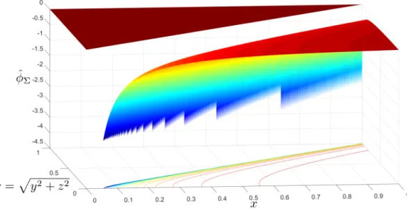
Σ, shown in Figure 2-7, is:
ˆ
𝜑
Σ(𝑥, 𝑦, 𝑧; 𝑀
∞) = −
1
2𝜋ℎ
Figure 2-7: Velocity Potential of a Supersonic Point Source
It is important to note that the velocity potential of a supersonic point source
is singular everywhere on its downstream Mach cone, not just at a single point as
it is in the subsonic case. Also, the disturbance from the supersonic point source is
restricted to inside the downstream Mach cone and does not affect the entire flow
field as in the subsonic case.
The velocity potential is imaginary everywhere outside of the Mach cones, so the
physical velocity potential can be obtained by taking the real part of the mathematical
velocity potential; however, the velocity potential is also real inside the upstream
Mach cone, so special care must be taken to discard the velocity potential for any
points upstream of the point source:
ˆ
𝜑
Σ(𝑥, 𝑦, 𝑧; 𝑀
∞) =
⎧ ⎪ ⎨ ⎪ ⎩−
1 2𝜋ℎ, 𝑥 > 𝛽
𝑃 𝐺√
𝑦
2+ 𝑧
20
, 𝑥 ≤ 𝛽
𝑃 𝐺√
𝑦
2+ 𝑧
22.7 Supersonic Z-Doublet
A supersonic z-doublet of strength 𝜅
𝑧can be used to represent lifting flow. The
velocity potential of a unit strength supersonic z-doublet ˆ𝜑
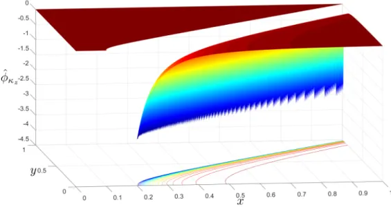
𝜅𝑧, shown in Figures 2-8
and 2-9, is obtained by taking the limit as the separation distance goes to zero of a
supersonic point source and sink each of strength Σ separated by a distance 𝑧 along
the z-axis while keeping the product Σ𝑧 = 1 constant.
Figure 2-8: Velocity Potential of a Supersonic Z-Doublet at 𝑧 = 0.1
Figure 2-9: Velocity Potential of a Supersonic Z-Doublet at 𝑦 = 0.1
potential of a unit strength supersonic point source:
ˆ
𝜑
𝜅𝑧(𝑥, 𝑦, 𝑧; 𝑀
∞) =
𝜕 ˆ
𝜑
Σ𝜕𝑧
=
𝜕 ˆ
𝜑
Σ𝜕ℎ
𝜕ℎ
𝜕𝑧
=
1
2𝜋ℎ
2−𝛽
2 𝑃 𝐺𝑧
ℎ
=
1
2𝜋
−𝛽
2 𝑃 𝐺𝑧
ℎ
3Again special care must be taken to discard the velocity potential of the supersonic
z-double outside of its downstream Mach cone:
ˆ
𝜑
𝜅𝑧(𝑥, 𝑦, 𝑧; 𝑀
∞) =
⎧ ⎪ ⎨ ⎪ ⎩ 1 2𝜋 −𝛽2 𝑃 𝐺𝑧 ℎ3, 𝑥 > 𝛽
𝑃 𝐺√
𝑦
2+ 𝑧
20
, 𝑥 ≤ 𝛽
𝑃 𝐺√
𝑦
2+ 𝑧
22.8 Infinitesimal Width Supersonic Horseshoe
Vor-tex
The infinitesimal width supersonic horseshoe vortex is equivalent to a semi-infinite
z-doublet line extending downstream along the x-axis from the origin. The velocity
potential for the unit strength infinitesimal width supersonic horseshoe vortex ˆ𝜑
Γ𝑧is obtained by integrating the velocity potential over the semi-infinite supersonic
z-doublet. In order to perform this integration, the hyperbolic radius needs to be shifted
by the integration variable 𝑥
′, which represents the location along the semi-infinite
z-doublet line:
ℎ(𝑥 − 𝑥
′, 𝑦, 𝑧; 𝑀
∞) =
√︁
(𝑥 − 𝑥
′)
2− 𝛽
2𝑃 𝐺
(𝑦
2+ 𝑧
2)
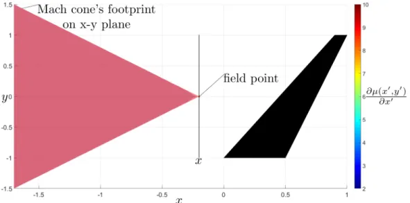
A field point located at (𝑥, 𝑦, 𝑧) only feels the influence from the portion of the
horseshoe vortex that is inside the field point’s upstream Mach cone. This can be
accounted for by truncating the horseshoe vortex, so the limits of integration along the
x-axis go from 0 to 𝑥 − 𝛽
𝑃 𝐺√
𝑦
2+ 𝑧
2. The intersection of the domain of dependence
of a field point with the plane of an infinitesimal width horseshoe vortex is shown in
Figure 2-10.
ˆ
𝜑
Γ𝑧(𝑥, 𝑦, 𝑧; 𝑀
∞) =
∫︁ 𝑥−𝛽𝑃 𝐺√
𝑦2+𝑧2 0ˆ
𝜑
𝜅𝑧(𝑥 − 𝑥
′, 𝑦, 𝑧; 𝑀
∞)𝑑𝑥
′=
−𝛽
2 𝑃 𝐺𝑧
2𝜋
∫︁ 𝑥−𝛽𝑃 𝐺√
𝑦2+𝑧2 0𝑑𝑥
′[(𝑥 − 𝑥
′)
2− 𝛽
2 𝑃 𝐺(𝑦
2+ 𝑧
2)]
3/2=
−𝛽
2 𝑃 𝐺𝑧
2𝜋
𝑥 − 𝑥
′𝛽
2 𝑃 𝐺(𝑦
2+ 𝑧
2)
√︁(𝑥 − 𝑥
′)
2− 𝛽
2 𝑃 𝐺(𝑦
2+ 𝑧
2)
⃒ ⃒ ⃒ ⃒ ⃒ ⃒ 𝑥−𝛽𝑃 𝐺√
𝑦2+𝑧2 0=
1
2𝜋
𝑧
𝑦
2+ 𝑧
2𝑥
√︁𝑥
2− 𝛽
2 𝑃 𝐺(𝑦
2+ 𝑧
2)
Figure 2-10: Velocity Potential Integration of an Infinitesimal Width Supersonic
Horseshoe Vortex
Note that the indefinite integral evaluated at the upper integration limit is infinite,
but this term is imaginary so it is discarded. The only restriction on the domain of
influence of the infinitesimal width supersonic horseshoe vortex is 𝑥 > 0. Redefining
ℎ
as the hyperbolic radius from the origin again, the potential of an infinitesimal
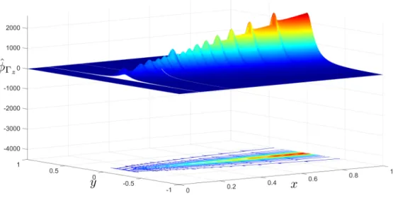
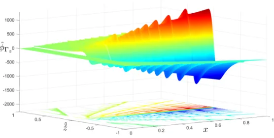
width supersonic horseshoe vortex, shown in Figures 2-11 and 2-12, becomes:
ˆ
𝜑
Γ𝑧(𝑥, 𝑦, 𝑧; 𝑀
∞) =
⎧ ⎪ ⎨ ⎪ ⎩ 1 2𝜋 𝑧 𝑦2+𝑧2 𝑥 ℎ, 𝑥 > 0
0
, 𝑥 ≤ 0
Figure 2-11: Velocity Potential of a Supersonic Infinitesimal Width Horseshoe Vortex
at 𝑧 = 0.1
Figure 2-12: Velocity Potential of a Supersonic Infinitesimal Width Horseshoe Vortex
at 𝑦 = 0.1
2.9 Tapered Supersonic Doublet Panel
In the present formulation, lifting surfaces will be represented by their mean camber
line and discretized into several doublet panels. These doublet panels will reside
entirely in the x-y plane and the slope of the mean camber line will only affect the
surface normal vectors of the control points used in the flow tangency boundary
condition. The side edges of the panels are required to be parallel to the freestream
direction, but the leading and trailing edges of the panels are allowed to be swept
at different angles. The doublet sheet strength 𝜇 will be constant along the leading
and trailing edge of each panel and will vary linearly in the streamwise direction.
For a doublet panel of this form, the leading edge (0) and trailing edge (1) lines are
expressed as:
𝑥
0(𝑦) = 𝑎
0+ 𝑏
0𝑦
𝑥
1(𝑦) = 𝑎
1+ 𝑏
1𝑦
and the doublet sheet strength, shown in Figure 2-13, as:
𝜇(𝑥, 𝑦) = 𝜇
0+
(𝜇
1− 𝜇
0)[𝑥 − 𝑥
0(𝑦)]
𝑥
1(𝑦) − 𝑥
0(𝑦)
Figure 2-13: Tapered Panel Doublet Sheet Strength
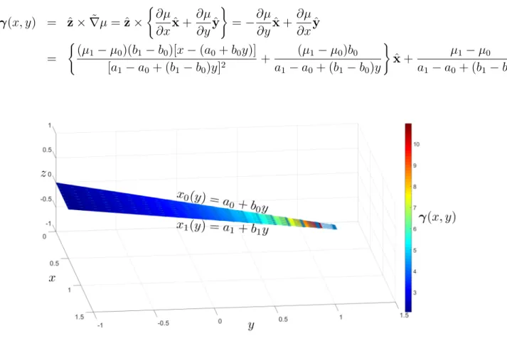
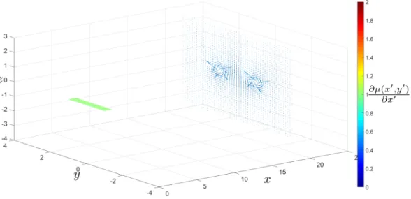
The vortex sheet strength vector 𝛾, shown in Figure 2-14, is defined as:
𝛾 = ˆ
n × ˜
∇𝜇
where ˜
∇𝜇
is the surface gradient of 𝜇.
Here the normal vector ˆn is required to be a unit vector, unlike in the flow tangency
boundary condition. Plugging in the above definitions of 𝜇, 𝑥
0, and 𝑥
1:
˜
∇𝜇(𝑥, 𝑦) =
𝜕𝜇
𝜕𝑥
x +
ˆ
𝜕𝜇
𝜕𝑦
y
ˆ
=
𝜇
1− 𝜇
0𝑎
1− 𝑎
0+ (𝑏
1− 𝑏
0)𝑦
ˆ
x −
{︃(𝜇
1− 𝜇
0)(𝑏
1− 𝑏
0)[𝑥 − (𝑎
0+ 𝑏
0𝑦)]
[𝑎
1− 𝑎
0+ (𝑏
1− 𝑏
0)𝑦]
2+
(𝜇
1− 𝜇
0)𝑏
0𝑎
1− 𝑎
0+ (𝑏
1− 𝑏
0)𝑦
}︃ˆ
y
For a panel in the x-y plane:
ˆ
n = ˆz
thus:
𝛾(𝑥, 𝑦) = ˆ
z × ˜
∇𝜇 = ˆ
z ×
{︃𝜕𝜇
𝜕𝑥
x +
ˆ
𝜕𝜇
𝜕𝑦
y
ˆ
}︃= −
𝜕𝜇
𝜕𝑦
x +
ˆ
𝜕𝜇
𝜕𝑥
y
ˆ
=
{︃(𝜇
1− 𝜇
0)(𝑏
1− 𝑏
0)[𝑥 − (𝑎
0+ 𝑏
0𝑦)]
[𝑎
1− 𝑎
0+ (𝑏
1− 𝑏
0)𝑦]
2+
(𝜇
1− 𝜇
0)𝑏
0𝑎
1− 𝑎
0+ (𝑏
1− 𝑏
0)𝑦
}︃ˆ
x +
𝜇
1− 𝜇
0𝑎
1− 𝑎
0+ (𝑏
1− 𝑏
0)𝑦
ˆ
y
Figure 2-14: Tapered Panel Vortex Sheet Strength Vector Field
The velocity potential of a tapered supersonic doublet panel with leading edge
doublet sheet strength 𝜇
0and trailing edge doublet sheet strength 𝜇
1at a field point
located at (𝑥, 𝑦, 𝑧) is calculated by integrating the expression for the potential of an
infinitesimal width supersonic horseshoe vortex over the panel span with the
appro-priate Γ
𝑧(𝑦)
. The infinitesimal width supersonic horseshoe vortex of strength Γ
𝑧(𝑦)
is equivalent to a z-doublet line of constant strength 𝜇, but since these panels do not
have constant doublet sheet strength in the streamwise direction, 𝜇 must be replaced
with
𝜕𝜇𝜕𝑥
and integrated over the streamwise length of the panel. This expression is
then integrated over the span of the panel. To perform this integration, 𝑥 must be
replaced with 𝑥 − 𝑥
′and 𝑦 must be replaced with 𝑦 − 𝑦
′, where (𝑥
′, 𝑦
′)
represents the
location within the panel. The 𝑥 limits of integration are from 𝑥
0(leading edge) to
𝑥
1(trailing edge) and the 𝑦 limits of integration are from 𝑦
0(left edge) to 𝑦
1(right
edge). The intersection of the domain of dependence of a field point with the plane
of a tapered supersonic doublet panel is shown in Figure 2-15. Note that the 𝑥 limits
of integration depend on 𝑦
′to account for the taper. The expression obtained from
evaluating this integral is omitted from this section due to its length and can be found
in appendix A.
𝜑(𝑥, 𝑦, 𝑧; 𝑀
∞) =
∫︁ 𝑦1 𝑦0 ∫︁ 𝑥1(𝑦′) 𝑥0(𝑦′)𝜕𝜇(𝑥
′, 𝑦
′)
𝜕𝑥
′𝜑
ˆ
Γ𝑧(𝑥 − 𝑥
′, 𝑦 − 𝑦
′, 𝑧; 𝑀
∞)𝑑𝑥
′𝑑𝑦
′=
1
2𝜋
∫︁ 𝑦1 𝑦0 ∫︁ 𝑎1+𝑏1𝑦′ 𝑎0+𝑏0𝑦′𝜇
1− 𝜇
0𝑎
1− 𝑎
0+ (𝑏
1− 𝑏
0)𝑦
′𝑧
(𝑦 − 𝑦
′)
2+ 𝑧
2𝑥 − 𝑥
′ √︁(𝑥 − 𝑥
′)
2− 𝛽
2 𝑃 𝐺[(𝑦 − 𝑦
′)
2+ 𝑧
2]
𝑑𝑥
′𝑑𝑦
′Figure 2-15: Velocity Potential Integration of a Tapered Supersonic Doublet Panel
A field point located at (𝑥, 𝑦, 𝑧) only feels the influence from the portion of the
tapered supersonic doublet panel that is inside the field point’s upstream Mach cone.
The velocity potential is imaginary everywhere outside of the field point’s Mach cones,
so the physical velocity potential can be obtained by taking the real part of the
mathematical velocity potential; however, the velocity potential is also real inside the
field point’s downstream Mach cone, so special care must be taken to discard the
velocity potential from any portions of the panel downstream of the field point. The
simplest way to do this is to truncate the panel downstream of the field point before
evaluating the superposition integral; however, this task is non-trivial and requires
the treatment of multiple cases.
Case 1
If the field point’s 𝑥 location is downstream of the entire panel, the integral can be
evaluated without modification.
𝜑(𝑥, 𝑦, 𝑧; 𝑀
∞)
=
1
2𝜋
∫︁ 𝑦1 𝑦0 ∫︁ 𝑥1(𝑦′) 𝑥0(𝑦′)𝜇
1− 𝜇
0𝑎
1− 𝑎
0+ (𝑏
1− 𝑏
0)𝑦
′𝑧
(𝑦 − 𝑦
′)
2+ 𝑧
2𝑥 − 𝑥
′ √︁(𝑥 − 𝑥
′)
2− 𝛽
2 𝑃 𝐺[(𝑦 − 𝑦
′)
2+ 𝑧
2]
𝑑𝑥
′𝑑𝑦
′Figure 2-16: Case 1
Case 2
If 𝑥 is upstream of a portion of the panel trailing edge, the panel must be divided
into two sections at the span location 𝑦
*such that:
thus:
𝑦
*=
(𝑥 − 𝑎
1)
𝑏
1On the side of 𝑦
*where the trailing edge of the panel is upstream of 𝑥, the integral
can be evaluated as is. On the other side, the upper 𝑥 limit needs to be changed from
𝑥
1to 𝑥 to truncate the panel downstream of 𝑥. There will now be two integrals, one
going from 𝑦
0to 𝑦
*and the other from 𝑦
*to 𝑦
1. Note that the integrand goes to zero
as 𝑥
′approaches 𝑥.
𝜑(𝑥, 𝑦, 𝑧; 𝑀
∞)
=
1
2𝜋
∫︁ 𝑦* 𝑦0 ∫︁ 𝑥1(𝑦′) 𝑥0(𝑦′)𝜇
1− 𝜇
0𝑎
1− 𝑎
0+ (𝑏
1− 𝑏
0)𝑦
′𝑧
(𝑦 − 𝑦
′)
2+ 𝑧
2𝑥 − 𝑥
′ √︁(𝑥 − 𝑥
′)
2− 𝛽
2 𝑃 𝐺[(𝑦 − 𝑦
′)
2+ 𝑧
2]
𝑑𝑥
′𝑑𝑦
′+
1
2𝜋
∫︁ 𝑦1 𝑦* ∫︁ 𝑥 𝑥0(𝑦′)𝜇
1− 𝜇
0𝑎
1− 𝑎
0+ (𝑏
1− 𝑏
0)𝑦
′𝑧
(𝑦 − 𝑦
′)
2+ 𝑧
2𝑥 − 𝑥
′ √︁(𝑥 − 𝑥
′)
2− 𝛽
2 𝑃 𝐺[(𝑦 − 𝑦
′)
2+ 𝑧
2]
𝑑𝑥
′𝑑𝑦
′Figure 2-17: Case 2
Case 3
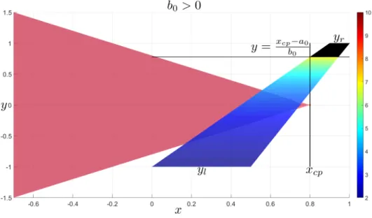
If 𝑥 is upstream of a portion of the panel leading edge, the 𝑦 limits of integration
must be changed to eliminate the section of the panel that is entirely downstream of
the field point. Either 𝑦
0or 𝑦
1needs to be changed to 𝑦
0*or 𝑦
* 1
such that:
𝑥
0(𝑦
0*) = 𝑥 = 𝑎
0+ 𝑏
0𝑦
*0𝑥
0(𝑦
1*) = 𝑥 = 𝑎
0+ 𝑏
0𝑦
*1thus:
𝑦
0*=
(𝑥 − 𝑎
0)
𝑏
0𝑦
1*=
(𝑥 − 𝑎
0)
𝑏
0𝜑(𝑥, 𝑦, 𝑧; 𝑀
∞)
=
1
2𝜋
∫︁ 𝑦* 𝑦0 ∫︁ 𝑥1(𝑦′) 𝑥0(𝑦′)𝜇
1− 𝜇
0𝑎
1− 𝑎
0+ (𝑏
1− 𝑏
0)𝑦
′𝑧
(𝑦 − 𝑦
′)
2+ 𝑧
2𝑥 − 𝑥
′ √︁(𝑥 − 𝑥
′)
2− 𝛽
2 𝑃 𝐺[(𝑦 − 𝑦
′)
2+ 𝑧
2]
𝑑𝑥
′𝑑𝑦
′+
1
2𝜋
∫︁ 𝑦*1 𝑦* ∫︁ 𝑥 𝑥0(𝑦′)𝜇
1− 𝜇
0𝑎
1− 𝑎
0+ (𝑏
1− 𝑏
0)𝑦
′𝑧
(𝑦 − 𝑦
′)
2+ 𝑧
2𝑥 − 𝑥
′ √︁(𝑥 − 𝑥
′)
2− 𝛽
2 𝑃 𝐺[(𝑦 − 𝑦
′)
2+ 𝑧
2]
𝑑𝑥
′𝑑𝑦
′Figure 2-18: Case 3
Case 4
If 𝑥 is upstream of the entire trailing edge, only one integral is needed with 𝑥 limits
from 𝑥
0to 𝑥.
𝜑(𝑥, 𝑦, 𝑧; 𝑀
∞)
=
1
2𝜋
∫︁ 𝑦*1 𝑦0 ∫︁ 𝑥 𝑥0(𝑦′)𝜇
1− 𝜇
0𝑎
1− 𝑎
0+ (𝑏
1− 𝑏
0)𝑦
′𝑧
(𝑦 − 𝑦
′)
2+ 𝑧
2𝑥 − 𝑥
′ √︁(𝑥 − 𝑥
′)
2− 𝛽
2 𝑃 𝐺[(𝑦 − 𝑦
′)
2+ 𝑧
2]
𝑑𝑥
′𝑑𝑦
′Figure 2-19: Case 4
Case 5
If 𝑥 is upstream of the entire panel, the potential at the field point is zero.
𝜑(𝑥, 𝑦, 𝑧; 𝑀
∞) = 0
Figure 2-20: Case 5
2.10 Perturbation Velocity Components
The perturbation velocity components of a tapered supersonic doublet panel are
ob-tained by taking the spatial derivatives of the velocity potential. These expressions
are omitted from this section due to their length and can be found in appendix A:
𝑢 =
𝜕𝜑
𝜕𝑥
𝑣 =
𝜕𝜑
𝜕𝑦
𝑤 =
𝜕𝜑
𝜕𝑧
One way to examine the validity of these expressions is to plot the perturbation
velocity component transverse to the x-axis in the y-z plane far behind the doublet
panel in the so called Trefftz plane. Here the panel should look like a single horseshoe
vortex in an incompressible flow.
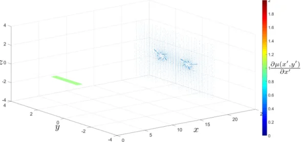
Far behind the doublet panel, only the integral vortex strength Γ
𝑧(𝑦
′)
matters.
The details in the variation of the doublet sheet strength over the chord of the panel
are not seen:
Γ
𝑧(𝑦
′) =
∫︁ 𝑥1(𝑦′) 𝑥0(𝑦′)𝜕𝜇(𝑥
′, 𝑦
′)
𝜕𝑥
′Since
𝜕𝜇(𝑥′,𝑦′)𝜕𝑥′
is inversely proportional to the chord, the integral vortex strength
Γ
𝑧is constant. Because Γ
𝑧is constant, when it is integrated across the span of the
panel, all interior vortex pairs cancel leaving only a single horseshoe vortex. This
holds for both non-tapered (Figure 2-21) and tapered (Figure 2-22) panels.
Figure 2-22: Tapered Panel Trefftz Plane Velocity
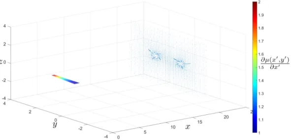
2.11 Woodward Vortex Panel Method
The Woodward method uses panels with a
𝜕𝜇(𝑥′,𝑦′)𝜕𝑥′
that is constant in the spanwise
direction, even for tapered panels. Since
𝜕𝜇(𝑥′,𝑦′)𝜕𝑥′
is constant spanwise, the integral
vortex strength Γ
𝑧is proportional to the local chord length in the spanwise direction.
Because Γ
𝑧is not constant, when it is integrated across the span of the panel, interior
vortex pairs do not cancel for tapered panels with different slopes at the leading and
trailing edges. The resulting Trefftz plane velocity is not that of a single horseshoe
vortex in this case.
Figure 2-23: Woodward Non-tapered Panel Trefftz Plane Velocity
Figure 2-24: Woodward Tapered Panel Trefftz Plane Velocity
The expressions plotted above in Figures 2-23 and 2-24 are from Woodward panels
having a constant
𝜕𝜇(𝑥′,𝑦′)𝜕𝑥′
in the streamwise direction. Woodward also uses vortex
panels with a linearly varying
𝜕𝜇(𝑥′,𝑦′)𝜕𝑥′
in the streamwise direction, but these still have
constant
𝜕𝜇(𝑥′,𝑦′)𝜕𝑥′
in the spanwise direction, so the results still do not represent a single
horseshoe vortex in the case of tapered panels with different leading and trailing edge
Chapter 3
Implementation
The matrix system that arises from the enforcement of the flow tangency boundary
conditions is derived. The supersonic doublet panel code that solves this matrix
system is described in detail. A method for calculating the aerodynamic coefficients
is presented. The numerical solutions of this code are compared to the analytical
solutions of four test cases.
3.1 Flow Tangency Boundary Condition
To evaluate the aerodynamic properties of lifting surfaces, the supersonic doublet
panel singularity strength parameters must be determined such that the flow tangency
boundary condition is satisfied at each control point:
V(𝑥
𝑐𝑝, 𝑦
𝑐𝑝, 𝑧
𝑐𝑝) ·
n(𝑥
𝑐𝑝, 𝑦
𝑐𝑝, 𝑧
𝑐𝑝) = 0
For steady flow at an angle of attack 𝛼 and sideslip 𝛽:
V(𝑥
𝑐𝑝, 𝑦
𝑐𝑝, 𝑧
𝑐𝑝) =
V
∞+
V
𝜇(𝑥
𝑐𝑝, 𝑦
𝑐𝑝, 𝑧
𝑐𝑝)
= 𝑉
∞cos(𝛼) cos(𝛽)ˆ
x − 𝑉
∞sin(𝛽)ˆ
y + 𝑉
∞sin(𝛼) cos(𝛽)ˆ
z
= 𝑉
∞(cos(𝛼) cos(𝛽) + 𝑢(𝑥
𝑐𝑝, 𝑦
𝑐𝑝, 𝑧
𝑐𝑝))ˆ
x + 𝑉
∞(− sin(𝛽) + 𝑣(𝑥
𝑐𝑝, 𝑦
𝑐𝑝, 𝑧
𝑐𝑝))ˆ
y
+ 𝑉
∞(sin(𝛼) cos(𝛽) + 𝑤(𝑥
𝑐𝑝, 𝑦
𝑐𝑝, 𝑧
𝑐𝑝))ˆ
z
Plugging the above expression for V into the flow tangency boundary condition
and dividing by 𝑉
∞yields:
[cos(𝛼) cos(𝛽) + 𝑢(𝑥
𝑐𝑝, 𝑦
𝑐𝑝, 𝑧
𝑐𝑝)]𝑛
𝑥+ [− sin(𝛽) + 𝑣(𝑥
𝑐𝑝, 𝑦
𝑐𝑝, 𝑧
𝑐𝑝)]𝑛
𝑦+[sin(𝛼) cos(𝛽) + 𝑤(𝑥
𝑐𝑝, 𝑦
𝑐𝑝, 𝑧
𝑐𝑝)]𝑛
𝑧= 0
Rearranging then yields:
𝑢𝑛
𝑥+ 𝑣𝑛
𝑦+ 𝑤𝑛
𝑧= − cos(𝛼) cos(𝛽)𝑛
𝑥+ sin(𝛽)𝑛
𝑦− sin(𝛼) cos(𝛽)𝑛
𝑧In this chapter, the freestream is no longer aligned with the x-axis. The axes will
be those used to specify the geometry of the aircraft.
3.2 Matrix System
The perturbation velocity components 𝑢, 𝑣, and 𝑤 depend linearly on the supersonic
doublet panel singularity strength parameter ∆𝜇 = 𝜇
1− 𝜇
0. Each panel contributes
to the perturbation velocity components of all the control points in its downstream
Mach cone. Let ˆ𝑢
𝑖𝑗be the contribution of the 𝑗
𝑡ℎpanel to the 𝑢 perturbation velocity
component of the 𝑖
𝑡ℎcontrol point per unit ∆𝜇. Using this notation, the above flow
tangency boundary condition can be written in matrix form:
[𝑛
𝑥𝑖𝑖𝑢
ˆ
𝑖𝑗+ 𝑛
𝑦 𝑖𝑖ˆ
𝑣
𝑖𝑗+ 𝑛
𝑧 𝑖𝑖𝑤
ˆ
𝑖𝑗]∆𝜇
𝑗= − cos(𝛼) cos(𝛽)𝑛
𝑥𝑖+ sin(𝛽)𝑛
𝑦 𝑖− sin(𝛼) cos(𝛽)𝑛
𝑧 𝑖The matrix [𝑛
𝑥𝑖𝑖𝑢
ˆ
𝑖𝑗+ 𝑛
𝑦 𝑖𝑖𝑣
ˆ
𝑖𝑗+ 𝑛
𝑧 𝑖𝑖𝑤
ˆ
𝑖𝑗]
is the supersonic AIC matrix. For this
system to have a unique solution, the number of control points must be equal to the
number of panels.
3.3 Supersonic Doublet Panel Code
The supersonic doublet panel MATLAB function calculates the following outputs:
supersonic doublet panel singularity strength parameters: ∆𝜇
velocity potential evaluated at control points: 𝜑
perturbation velocity components evaluated at control points: 𝑢, 𝑣, and 𝑤
And requires the following inputs:
𝑥, 𝑦, and 𝑧 coordinates of the control points: (𝑥
𝑐𝑝, 𝑦
𝑐𝑝, 𝑧
𝑐𝑝)
𝑥, 𝑦, and 𝑧 components of the control point normal vectors: (𝑛
𝑥𝑐𝑝, 𝑛
𝑦 𝑐𝑝, 𝑛
𝑧 𝑐𝑝)
𝑦 coordinates of left and right panel side edge: (𝑦
𝑙, 𝑦
𝑟)
𝑥 coordinates of left leading edge, left trailing edge, right leading edge, and right
trailing edge panel corners: (𝑥
𝑙,𝑙𝑒, 𝑥
𝑙,𝑡𝑒, 𝑥
𝑟,𝑙𝑒, 𝑥
𝑟,𝑡𝑒)
flow angles: 𝛼 and 𝛽
flow Mach number: 𝑀
∞function
[dm ,phi ,u,v,w] = supersonic_doublet_panel (
x_cp_vec , y_cp_vec ,
...
z_cp_vec ,n_x_cp ,n_y_cp ,n_z_cp , y_l_vec , y_r_vec ,
x_l_le_vec , x_l_te_vec ,
...
x_r_le_vec , x_r_te_vec ,alpha ,beta ,M)
The first step is to calculate the Prandtl-Glauert factor 𝛽
𝑃 𝐺, not to be confused
with the sideslip angle 𝛽, and the geometric coefficients 𝑎
0, 𝑎
1, 𝑏
0, and 𝑏
1. The
supersonic Prandtl-Glauert factor is defined as:
𝛽
𝑃 𝐺=
√︁