Testing techniques and forecasting ability of FX Options Implied Risk Neutral Densities

(1)

Testing techniques and forecasting ability of FX Options Implied Risk

Neutral Densities

(2)

Abstract

The purpose of this paper is to test and compare two methods to extract implied risk neutral density from Tel-Aviv Stock Exchange (TASE) traded option prices on the exchange rate between the US dollar and the New Israeli Shekel (NIS). The compared methods in this paper are the two lognormal mixture (parametric approach) and Shimko's methods (non-parametric approach). The comparison is done in terms of their ability to provide implied densities having a goodness of fit of theoretical to observed option prices, robustness to various pricing errors and their ability to generate reasonable density forecast. It has been found that Shimko's method is a preferable method for these tasks. However, it may be unstable when providing goodness of fit of theoretical to observed option prices.

(4)

Introduction

In recent years an entire literature on methods of extracting implied probability density functions of future returns of an underlying asset has been developed. Central Banks, Risk Managers and institutional investors use densities implied from option prices to have a better understanding of uncertainty regarding future returns. For example: the Bank of Israel uses implied densities to evaluate the likelihood of future possible fluctuations in the exchange rates between the Dollar and the New Israeli Shekel (NIS) as a part of decision making regarding interest rates.

The Bank of Israel uses these implied densities to calculate, on daily basis, the probabilities of 5% depreciation and appreciation in one month of the NIS against the dollar. These probabilities and other statistics (such as the skewness and kurtosis) help to have a better understanding of the governing trend in the exchange rate between the dollar and NIS. Information regarding this exchange rate is important because Israel is a small open economy where fluctuations in the exchange rate have a strong impact on the Israeli Consumer Price Index (CPI). Therefore, it is important for the Bank of Israel to have a deeper understanding of exchange rates risk which is allowed using the implied densities.

Implied densities are also valuable for forecasting. For example: the mean of an implied density can be used as a point forecast of the asset price in the future with a better understanding and information regarding the uncertainty of this forecast. They can also provide a forecast range within a given percentile. For an option trader this is most important for choosing the correct trading strategy.

The advantage of using traded option prices for understanding future possible returns is that these financial assets are forward looking by their nature. The price of an option embodies expectations about the future.

Since option and other derivative markets have become deep and liquid enough for trading in the last thirty years, their embedded information regarding the future has

(5)

become more and more reliable and relevant. Furthermore, their link to their respective underlying security market (which is explicitly expressed in the Black & Scholes formula) enables them to absorb news and new information quickly and to embed further information that is not contained in the cash market.

The main problem with constructing implied densities is that there is no consensus about how to extract them. Another problem is that they are usually derived under the assumption that the market is risk neutral and it is hard to determine the risk premium if this assumption fails. Therefore, they fail to take into account the market's attitude towards risk. Thus, using these implied densities may be problematic from the point of view of interpreting market uncertainty. Interpreting market uncertainty under the risk neutral measure might lead to false conclusions if the unobserved risk premium is significant enough.

Chart A gives an example of the intraday trajectory of the price of an option on the TA25 index (the Tel-Aviv 25 stock index) and the index1 itself on July 16th, 2006. This chart illustrates the close link between derivative and the underlying markets. Note that the price of the call option changes almost in parallel to the level of the TA25 index.

Chart A: Intraday trajectory of the TA25 index and the price (in NIS) of a European call option with a strike price of 780 and 30 days to expiry.

1 _{Intraday data of the TA25 stock index are available for download at the Tel – Aviv Stock Exchange}

internet site (www.tase.co.il). Unfortunately, the intraday trajectory of the exchange rate between the U.S dollar and the New – Israeli shekel (The options dealt in this paper) are unavailable.

200 400 600 800 1000 1200 1400 1600 1800 09 :3 0 09 :4 3 09 :5 6 10 :0 9 10 :2 2 10 :3 5 10 :4 8 11 :0 1 11 :1 4 11 :2 7 11 :4 1 11 :5 4 12 :0 9 12 :2 3 12 :3 7 12 :5 3 13 :0 7 13 :2 1 13 :3 7 13 :5 3 14 :0 9 14 :2 8 14 :4 3 14 :5 6 15 :0 9 15 :2 2 15 :3 5 15 :4 8 16 :0 1 16 :1 4 690 700 710 720 730 740 750 760 770 780 Call Option

(6)

The aim of this paper is to examine and compare two methods for obtaining implied risk neutral densities. The implied densities will be obtained from options traded at the Tel-Aviv Stock Exchange (TASE) on the exchange rate between the U.S dollar and the New Israeli Shekel (NIS).

Thus, this paper in some ways serves as a continuation of R. Stein's (2003&2004) work on implied densities from options on the exchange rate between the U.S dollar and the NIS. In his work, R. Stein presented two methods for extracting implied densities from option prices. The first method is based on a parametric assumption of the underlying exchange rates dynamics. The second method, which also deals with the expected future evolution of exchange rates, is not based on any parametric assumption.

In this paper I will examine and compare three aspects of these two. First I compare how accurate these methods are in creating theoretical option prices that are close to those observed in the market. Note that the theoretical price of an option depends on some probability density function. This will test how well does the obtained implied density (given the method to obtain it) is for pricing options and other derivative products. The second aspect is the robustness of implied densities to various unobserved mistakes in the data using a Monte Carlo based procedure proposed by R.Bliss and N.Panigirtzoglou. Finally, we compare both methods ability to obtain a reliable forecast of the probability density function of future underlying asset returns.

This paper is divided into five sections. The first section describes the data. The second describes the two methods for obtaining the implied risk neutral densities from option prices. The third describes the three tests on these implied densities. The fourth presents the results and the fifth section concludes this paper.

(7)

I. The

Data

The data covers the period from January 4th 2004 to November 30th 2005, and are taken from the TASE quote book. The quotes are a snapshot of trade at around 14:00 PM, where most transactions take place and therefore it is the time of the day where the market is most active. The choice of these quotes rather then closing price is due to liquidity issues, since closing option price data have a higher average Bid - Ask spread than mid day prices. In this section I will discuss my criteria for option selection, and my choice of using implied spot prices instead of quoted spot prices. As a proxy for the risk-free rate, I use the yield on the relevant time to maturity Israeli zero – coupon bond2. As a proxy for the foreign risk free rate I use the yield on a relevant time to maturity LIBOR3 rate on the US dollar.

1. Criteria for option selection

The first criterion I consider relates to the quoted Bid – Ask spread of traded options. This spread might be a major source of error, when extracting information from option prices. Since the average of the Bid and Ask prices is used as a proxy for the observed price of the option, it is desirable to have a narrow spread, which reduces uncertainty. An additional issue in option selection is “moneyness”. Taking options that are too much out of the money can lead to negative probabilities and outliers when calculating the implied volatility. A third issue concerns the time to maturity, which I chose to vary from 21 days to 62 days. It has been found out that traded options at these maturities are most liquid in terms of trading volumes and therefore bearing a price which may be more reasonable than shorter term maturities. Option selection in this research paper involves three steps:

• Step 1: Choose options with quoted Bid-Ask such that:

, , , ,

, ,

i t i t i t i t

i t i t _t

Bid Ask Bid Ask E Ask Ask ⎛ ⎞ − − ≤ ⎜_⎜ ⎟_⎟ ⎝ ⎠ )

2_{Also known as the MAKAM – Israeli Short term lending rate.}

3_{The London Interbank Offered Rate – An interest rate at which financial institution can borrow funds}

from other banks in the London interbank market. It is used as a benchmark for short term interest rates on the Dollar, Euro and other major currencies.

(8)

Where:

Bidi,t , Aski,t – Quoted Bid and Ask of the i’th option at time t

t t i t i t i Ask Ask Bid E _⎟⎟ ⎠ ⎞ ⎜⎜ ⎝ ⎛ − , , ,

) - Daily average of relative difference between bid and ask. This

step comes in place in order to omit from the sample the most illiquid options. On average, the daily average of relative difference between bid and ask is around 100%

• Step 2: Omit options with annual implied volatility higher than 20% (too far

out of the money).

• Step 3: Choose options with time to maturity ranging between 21 to 62 days.

2. Use of implied spot rates instead of quoted spot rate

One important aspect of FX option trading in Israel is that trading takes place on Sundays when there is no trade on the underlying asset (The US dollar)4. This can cause a problem for extracting information from option prices. Furthermore, the dollar spot market has changed considerably within the sample period5. As a result, intraday movements of the dollar against the NIS have been more frequent, causing an amplification of errors due to non-synchronicity between the option and its underlying markets. This means that the price of an option may not reflect the latest available price of the underlying.

Chart 1 and Table 1, which show the squared deviation between the price implied from the Put – Call parity equation and quoted market spot price illustrates the problem of non - synchronicity between the derivative and the underlying markets. This non-synchronicity has important implications for the implied distribution6. When using the non-parametric method, an unusual thick tailed density is obtained while with the parametric method, the mean of the distribution is affected. Throughout the sample

4_{On Sundays, the TASE uses the dollar rate which is determined on Friday 13:00PM as the underlying}

asset price.

5_{Within that period support bands for exchange rate between the NIS and dollar were removed, making the}

NIS completely a floating currency. Also, the "Bachar" reform decentralizing Israeli capital markets has contributed to an increase in flows of fund into and out of Israel.

(9)

period, I will use the implied spot rate instead of quoted market spot rate7 . As the chart and table illustrate, the option market is somewhat close to being a complete market. If the squared deviations between the implied and quoted exchange rate were significant than it would suggest that the options on the dollar market was incomplete or had some market failure.

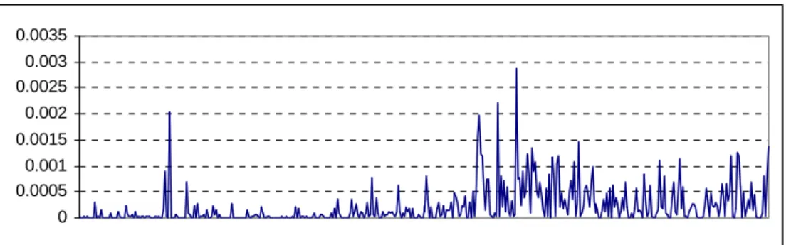
Chart 1: The Squared deviation between implied from Put-Call parity spot rate and the quoted market spot rate: 4/1/2004 – 30/11/20058

0 0.0005 0.001 0.0015 0.002 0.0025 0.003 0.0035

Table 1: TheSquared deviation between implied from Put-Call parity spot rate and the quoted market spot rate: 4/1/2004 – 30/11/20059

All days excluding Sundays

All days included in the Sample data Series 0.12 0.18 Mean 0.1 0.036 Median 0 0 Min 1.51 1.51 Max 0.19 0.22 Standard Deviation

7_{See Annex 2 on option selection criteria for obtaining the implied spot}

8_{Within that time the dollar varied from 4.522NIS/1$ on April 1}st_{2004 to 4.661NIS/1$ on October 11}th

2005, with estimated 6% historical volatility.

(10)

II. Extracting the implied risk neutral PDF from option prices

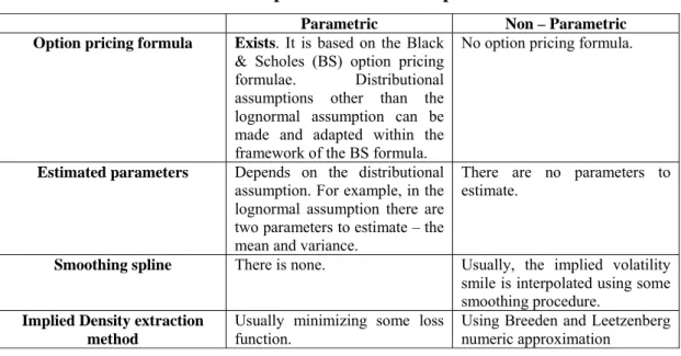
This section describes two different methods for extracting implied risk neutral densities from option prices. Generally speaking, there are two main schools of thought regarding the extraction of these densities: the “parametric school” and the “non-parametric school”. In the parametric school, the underlying security prices are assumed to follow some particular distribution (e.g. the log-normal). In the second, non-parametric school, no such assumptions are made. The table below summarizes the main differences regarding these two approaches. In this paper, I use a mixture of two lognormals (2LN) for the parametric method. For the non-parametric method, we shall extract the implied density using an approach devised by Shimko (1993).

Table 2: Main characteristics of parametric and non-parametric methods

Parametric Non – Parametric

Option pricing formula Exists. It is based on the Black

& Scholes (BS) option pricing formulae. Distributional assumptions other than the lognormal assumption can be made and adapted within the framework of the BS formula.

No option pricing formula.

Estimated parameters Depends on the distributional

assumption. For example, in the lognormal assumption there are two parameters to estimate – the mean and variance.

There are no parameters to estimate.

Smoothing spline There is none. Usually, the implied volatility

smile is interpolated using some smoothing procedure.

Implied Density extraction method

Usually minimizing some loss function.

Using Breeden and Leetzenberg numeric approximation

1. The two lognormal mixture assumption

The 2LN assumption has been widely used to extract information from option prices. Bahra (1997) applies this method while studying the implied information from 3-month Sterling interest rate options and LIFFE equity index options. Gemmill and Saflekos (1999) use this method to examine the usefulness of implied probabilities extracted from options on the FTSE100. Stein and Hecht (2003,2004) applied this method on options on the exchange rate between the US dollar and the New Israeli Shekel (as I will do here).

(11)

A mixture of two-lognormals has some advantages when applied to currency options. It is applicable when there is not too wide a range of strike prices available (when there are no options traded far away from the money). It is computationally easy. Estimation is relatively simple since there are only five parameters to estimate. Moreover, a mixture of two lognormal distributions is reasonably empirically reliable. However, there are some drawbacks. For example, the implied distribution may exhibit spikes due to outliers in observed option prices or misspecification of the mixture distribution. Also, it may be too restrictive as an assumption for the dynamics of exchange rates since the governing law of exchange rate fluctuations is unknown and perhaps a more general distribution such as the Generalized Beta of the 2nd type (GB2) is more adequate.

Under the above assumption, the price of a European put or call option is basically a linear combination of two Black and Scholes10_{option prices related to two different}

states of the world.

) , ( ) 1 ( ) , ( ) , (K τ θC₁ K τ θ C₂ K τ C = BS + − BS ₍₁₎ where BS

C1 denotes the Black and Scholes price of a European call in state 1,

BS

C2 is the price in state 2 and θ is the probability of the first state. More explicitly, the prices a European put and call options will be:

[

]

T T K T T rt dS X S S L S L e K C( ,τ)= −

∫

+∞θ (α₁,β₁; )+(1−θ) (α₂,β₂; )( − ) (2a)

[

]

T T K T T rt dS S X S L S L e K P( , ) ( , ; ) (1 ) ( , ; )( ) 0 1 1 + − 2 2 − = −

∫

_θ _α _β _θ _α _β τ , (2b) where L(α,β;S_T)= 1 STβ 2π e −(ln ST−α )2 2β2

10_{Since I study options on exchange rates I use the Garman-Kohlhagen formula:}

) ( ) ( ₁ τ ₁ σ τ τ ₋ ₋ = − − d N Ke d N e S C rf rd

(12)

is the lognormal density and τ σ μ α ⎟ ⎠ ⎞ ⎜ ⎝ ⎛ ₋ + = 2 2 1 ln _i _i i S and βi =σi τ . (3)

Elementary calculations, using the Black and Scholes pricing formula yield the following theoretical option prices for a European put or call:

C(K,τ)= θ e−rdt_eα1+0.5β12_N(d 1)− e −rft KN(d2)

[

]

+ (1−θ) e−rdt_eα2+0.5β22 N(d3)− e −rft KN(d4)

[

]

{

}

(4a) P(K,τ)= θ−e−rdt_eα1+0.5β12_N(−d 1)+ e −rft KN(−d2)

[

]

+ (1−θ)−e−rdt_eα2+0.5β22_N(−d 3)+ e −rft KN(−d4)

[

]

{

}

(4b) Where: 1 2 1 1 1 ln β β α + + − = K d ,d2 = d1−β1 , 2 2 2 2 3 ln β β α + + − = K d and d4 = d3 −β2 (5)

Note that the above prices are closed-form solutions of equations (2a) and (2b), as proved by Bahra (1997). In order to obtain an implied PDF based on an empirical observation of the option prices, we may minimize their relative squared deviation from the theoretical option prices implied by the 2-lognormals mixture distribution, or

α1,α2,β1,β2,θ

Min

Ci ^ − C(K_i,τ) C(K_i,τ) ⎡ ⎣ ⎢ ⎢ ⎤ ⎦ ⎥ ⎥ 2 + Pi ^ − P(K_i,τ) P(K_i,τ) ⎡ ⎣ ⎢ ⎢ ⎤ ⎦ ⎥ ⎥ 2 j=1 m

∑

i=1 n

∑

⎧ ⎨ ⎪ ⎩ ⎪ ⎫ ⎬ ⎪ ⎭ ⎪ , (6) where ₍ _,_τ_), ₍ _,_τ₎ i i P K K

C are the observed market prices for a given strike price (Ki) and

time to maturity (τ) _C),_P) are the implied theoretical prices and

{

_α₁,_α₂,_β₁,_β₂,_θ

}

are the parameters of the 2LN distribution to be estimated.

(13)

The optimization problem above is the same as in Stein and Hecht's work. I have tried other optimization problems, notably the one used by Bahra and other researchers, which has the following form

α1,α2,β1,β2,θ

Min

C(Ki,τ)− Ci ^ ⎛ ⎝ ⎜ ⎞ ⎠ ⎟ 2 + P(Ki,τ)− Pi ^ ⎛ ⎝ ⎜ ⎞ ⎠ ⎟ 2 j=1 m

∑

+ θeα1+ 1 2β1 2 + (1−θ)eα2+ 1 2β2 2 − erτ S ⎛ ⎝ ⎜ ⎞ ⎠ ⎟ 2 i=1 n

∑

⎧ ⎨ ⎪ ⎩ ⎪ ⎫ ⎬ ⎪ ⎭ ⎪ (7)

The third term of the optimization equation constrains the parameters such that the third term is equal to the theoretical forward spot rate. However, I found that optimizing over the above equation gives unsatisfactory parameter estimates. The functional form of equation (6) is more stable11 and also has the advantage of being somewhat less sensitive to starting values.

2. A volatility “smile” based approach to extract implied PDF

Unlike the parametric approach which assumes distribution, the nonparametric approach derives the implied PDF directly from the second derivative of the theoretical12 option price with respect to its strike price. The distribution is obtained by interpolating the volatility smile of the call option price directly by fitting a spline and expressing implied volatility as a function of the strike price. Then, using Breeden and Leetzenberg approximation for the second derivative of option price with respect to strike price, we obtain the implied risk neutral density.

Bates (1991) for example, fits a cubic spline on S&P 500 options when studying the relative predictive capabilities of implied distributions before and after the 1987 Wall Street crash. Shimko (1993) fits implied volatility to strike prices and grafts the tails of a lognormal distribution to the implied distribution. Malz (1997) follows Shimko’s

11_{More stable in the sense that if the optimization is repeated 'n' times (with same values and sample data),}

results will not vary by much.

12_{For a call:}

∫

+∞ − ₋ = K t T t rt t K r t e S K p S dS S C( , , , ) ( ) ( ) .

(14)

approach, but interpolates volatility smile across options deltas13’ while Bliss, Panigirtzoglou and Syrdal (2002) use a natural spline technique to fit implied volatilities to option deltas. Ait – Sahalia and Lo (1998) use kernel regressions to express the relationship between the option price and the strike price.

Many other smoothing techniques are used to improve and to confront essential issues raised in the application of the non-parametric approach. The first issue relates to most accurately fitting implied volatility given relatively small number of observations. The second issue is the presence of outliers in implied volatility at options which are far out or in the money. These outliers usually appears for reasons due to lack of liquidity (measured in terms of low trading volumes and relatively large bid and ask spreads) and option miss-pricing.

The Breeden and Leetzenberger approach starts by using a butterfly spread. This spread replicates a state contingent claim (or Arrow-Debreu security). It consists of a short position in two calls with exercise prices of Ki (At The Money Options) and a long

position in two calls, one with a strike price of Ki + Δ Ki and the other with a strike price

of Ki - Δ Ki. The payoff of this portfolio will be 1 for X = Ki and 0 otherwise.

1 )] , ( ) , ( [ )] , ( ) , ( [ ₌ Δ Δ − − − − Δ + =K_i X i i i i i i i K K K C K C K C K K C τ τ τ τ (7)

As ΔKi approaches to0, the limit of the butterfly spread becomes a replication of an

Arrow – Debreu security. If we let P(Ki,τ;ΔKi) be the price of such a claim centered at X

= Ki and divided by ΔKi, we obtain a second order difference quotient:

2 ) ( )] , ( ) , ( [ )] , ( ) , ( [ ) ; , ( i i i i i i i i i i K K K C K C K C K K C K K K P Δ Δ − − − − Δ + = Δ Δ τ τ τ τ τ (8) And For X = Ki: i i i X K i i K X X C K K K P = → Δ = Δ Δ 2 2 0 ) , ( ) ; , (

lim

τ ∂ _∂ τ (9)

(15)

Now, since the price of an Arrow-Debreu security is an expression of the present value of $1 multiplied by the risk neutral probability of a state occurring at X = Ki we have the

following estimate of the risk neutral density f(ST):

) ( , ) ( 2 ) ( ) , ( 2 1 1 2 2 i i i i i i T r K C C K C C C S f e K K C ₌ Δ − + = ≡ −τ + − ∂ τ ∂ ₍₁₀₎

Prior to applying the Breeden and Leetzenberger result however, we need to fit a volatility smile in order to obtain a set of synthetic option prices on a continuum within a given range of strike prices. Shimko's method for fitting the implied volatility is considered below.

Shimko's approach

In order to obtain call14 prices as a function of strike prices, Shimko fits a quadratic equation to implied-volatility15 with parameter coefficients estimated using a simple OLS procedure. σi IV =β 0+β1Ki+β2Ki 2₊_ε i (11)

Thus we obtain a fitted functional form of implied volatility with respect to the strike price and the price of a synthetic call option is represented by equation 12. Using this equation, we can apply equation 10 in order to estimate the implied risk neutral distribution. Ci synthetic _{= C}BS_(S 0,Ki,τ,rf,rd,σi IV_(K i)) (12)

In his work, Shimko, assumes (as a matter of convenience) that the tails of his non-parametric density are similar to the tails of the lognormal distribution and therefore grafts onto the non-parametric distribution. Alternatively, to obtain the tails, synthetic call

14_{Put prices are translated to call prices using the Put-Call Parity equation.}

15

Implied volatilities are extracted from observed option prices using Newton-Raphson algorithm. This algorithm is implemented using VBA Excel.

(16)

prices can be calculated outside the strike price range. In this paper, the tail of the non-parametric distribution are not assumed nor calculated from synthetic call prices. The reason for this is that calculating the tails of distribution usually generated negative or unreasonable probabilities. Furthermore, assuming log normal tails in the case of TASE traded option is not sound due to low trading volumes in far out and in the money options.

III. Testing implied densities

In this paper, we consider tests for: Stability/Robustness, Goodness of fit of synthetic option prices to observed option prices and the forecasting ability of implied densities. For Goodness of fit I compare observed and synthetic option prices using the Mean Squared Error (MSE). For stability (or robustness to errors in the data), I apply the algorithm by Bliss and Panigirtzoglou. Finally, to test forecasting ability I use the Probability Integral Transform (PIT) test on the estimated implied densities. These tests can be used to evaluate and compare parametric and non-parametric methods for extracting implied risk neutral densities.

1. Goodness of fit comparison

Goodness of fit over the sample period is compared between Shimko’s and 2LN approach. For each day the mean squared error (MSE) between market and theoretical/synthetic prices were calculated by:

(

)

∑

− − = Nk i t observed t K t C C N MSE ˆ 2 1 1 (14)

I study the time evolution of this statistical indice. Note that on a given day, one method might do a better job in fitting synthetic prices to real prices than the other. Thus, to rank and compare the two approaches used, we shall also use "time" scores, which count: the number of times (or days) where one approach is a better fit than the other. In addition, I calculate the time series mean and variance. These comparisons will allow a better understanding of these methods.

(17)

2. Bliss & Panigirtzoglou test for robustness

R. Bliss and N. Panigirtzoglou (henceforth, BP) analyzed the robustness to price errors of various methods for extracting implied densities. Such pricing errors can be detected using put/call parity equation and the convexity of option prices with respect to strikes. However, the pricing error's source cannot be determined. BP mentioned the following possible sources of errors that might arise with traded options data:

(1) Errors occurring while recording option prices (human errors), (2) Non – synchronicity between options and their underlying prices,

(3) Differential (undetected) liquidity premia between option prices and their respective strikes (out and in of the money options tend to be less liquid than at the money options).

A Robustness test is performed using a Monte Carlo procedure. The algorithm, adapted to TASE traded dollar currency options, consists of the following:

1. Option prices across all strikes are “disturbed” by a uniformly distributed error on an interval centered around zero and with length equal to half a tick. In the context of the TASE traded options, tick size is determined according to the following manner:

• 1 NIS for an option traded at a price up to 20 NIS

• 5 NIS for an option traded at a price between 20 – 200 NIS • 10 NIS for an option traded at a price between 200-2000 NIS • 20 NIS for an option traded at more than 2000 NIS

2. For each method, an implied density is extracted and the median, the mode and inter – quartile range are calculated.

(18)

Such simulation provides a large number of series (100 for each method) which can be used to compare the estimation methods. The standard deviation, variance, range, mean and the median of the squared difference between the “true” and “disturbed” indices was calculated. On the basis of these results, the method that provides the series with the lowest deviation indicators will be considered the most robust.

In their paper, BP, perform the test on traded options on the Short Sterling interest rate and the FTSE100 in order to compare the 2LN and their own non-parametric method. They conclude that their non-parametric method is more robust to errors in pricing. In addition, they observe neither method is robust in the tails of the distribution (the 1st and 99th percentiles of the implied density). Their results are explained by the fact that the 2LN approach has assumptions limiting the shape of the implied risk neutral density and thus it is more sensitive to pricing errors.

In this paper, I test robustness for each method using option prices observed on May 26th, 2005. This is due to numerical limitations of the hardware that is used: without such limitations, I would have conducted this test over the whole sample data, giving a better understanding of how robust these two methods are. Furthermore, I selected only three empirical statistical indices due to the fact that the non – parametric density estimated is with no tails and thus only empirical indices can be obtained from it (such as the median, the mode and interquartile range, The mean, variance and higher moments are not calculated).

3. Probability Integral Transformation

The PIT directly relates the true PDF to the implied PDF extracted from option prices, and might be more informative in comparing between parametrically and non-parametrically obtained distributions. The PIT evaluates the forecasting ability of the implied distribution. It can be used to test both the tails of the underlying distribution as well as the whole distribution. In this paper, since the tails of the distribution are not estimated in the non-parametric derived implied density, I will focus on the whole implied distribution.

(19)

Tests based on the PIT for evaluating estimated density forecast dates back as early as 1952 (Rosenblatt). However, only recently it has been applied as a test for the accuracy of implied risk neutral densities. Diebold, Gunther and Tay (DGT, 1998) give a detailed examination of this methodology while applying it to a simulated GARCH process. They also indicate its potential use on a wide range of financial models, such as value at risk.

Anagnou et al. (ABHT, 2002) applied this method on density forecasts of the S&P 500. In their research, they evaluate three parametric approaches (GB2, Negative Inverse Gaussian and the two-lognormals mixture) and a single non-parametric approach based on the B – Spline. They conclude that the implied risk neutral PDF is a poor forecast of future prices.

Craig, Glatzer, Keller and Scheicher (CGKS, 2003) tested implied densities obtained from options on the DAX indices (extracted using the two lognormal approach). Their results point to evidence of strong negative skewness as well as a “significant difference

between the actual density and the risk neural density". They conclude: “market participants were surprised by the extent of both the rise and fall of the DAX”.

Alonzo, Blanco and Rubio (2005) derive implied densities from options on the IBEX35, also using a parametric and a nonparametric procedure. Using data from 1996 until 2003, they cannot reject the hypothesis that implied densities successfully forecast future realizations. Nevertheless, they found that this result is not robust within sub periods.

Gurkaynak and Wolfers (GW, 2005) apply the PIT on implied densities derived from Macroeconomic Derivatives. They conclude after a series of graphical tests, that these densities are accurate forecasts. They mentioned that this result is rather surprising, since asset prices usually tend to include a risk premium. When there are unobserved risk premia, options priced in a risk neutral world tend to be systematically biased.

The PIT test consists of determining whether the density forecast is equal to the realized future density. At first, this sounds impractical and unfeasible since the density cannot be

(20)

observed, even ex post. There are a few important notions that should be kept in mind in such a case. First, a density forecast is basically a distribution of many possible point forecasts. Therefore, moments of implied distribution give a description of potential future point realizations—since only one realization is possible.

DGT point out that it is possible to establish a relationship between the data generating process and the sequence of density forecasts through the probability integral transform of realized returns (in this paper I refer to the realized exchange rate between the U.S Dollar and NIS)with respect to the forecasts obtained.

) ( ) ( _t _t y t t p u du P y z t = =

_∫

∞ − (17)

Where: p_t(u)is the estimated density forecast, P_t(y_t) is the corresponding estimated

cumulative density function, y is the realization itself and _t z is the probability integral t

transform. DGT prove that zt follows the following statistical law:

zt ~ i.i.d

Uniform(0,1) (18)

Since the non-parametric implied density is restricted to a range of strike prices (and thereby truncated), calculation of the PIT for both densities can be done in a manner similar to that of ABHT. This will restrict the PIT test to the body of the distribution and allows a comparison between the two implied densities.

zt

*₌ Pt(yt)− Pt(Kmin,t)

P_t(K_{max t})− P_t(K_min,t)

In order to test the (null) hypothesis that the risk neutral density is an accurate forecast (the PIT, zt, follows a Uniform distribution), I used the procedure of Christoffersen and

(21)

Mazotta (CM, 2004). In their paper, they test unconditional and conditional normal distributions of the following transformation of the PIT:

xt = Φ

−1_(z

t) ~ i.i.d

N(0,1) (19)

In this paper, testing unconditional normality will be done because the tails of the non-parametric density are unknown and therefore the mean, variance and higher moments cannot be calculated.

To test the unconditional normality of xt, we use the following joint hypothesis:

E(xt)= 0 E(x_t2)=1 E(xt 3₎_{= 0} E(xt 4₎_{− 3 = 0}

Using GMM16 in order to allow autocorrelation from overlapping observations, we estimate a system of four equations and test for the significance of the coefficients a1, a2,

a3 and a4: xt = a1+ et (1) xt 2_{−1= a} 2+ et (2) x_t3= a3+ et (3) xt 4_{− 3 = a} 4+ et (4 )

This test is a slight modification of the Berkowitz test and it is performed to allow overlap in the data and as a result an increase in the sample size.

16_{The GMM procedure is run by using EVIEWS software. There is a restriction relating to autocorrelation}

(22)

IV. Results

This section will present the results obtained from the tests on the obtained implied densities. It is divided into four sub sections. The first part will present the results of the goodness of fit comparison; the second part presents results for the Bliss & Panigirtzoglou robustness test; the third part presents results for the truncated version of the probability integral transform tests and the forth part will conclude.

1. Goodness of fit comparison

The chart and table below show the daily evolution of MSE (as defined in equation 14) of both synthetic derived option prices and their respective summary statistics.

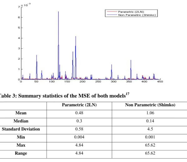
Chart 2: MSE of both synthetically derived option prices

Table 3: Summary statistics of the MSE of both models17

Parametric (2LN) Non Parametric (Shimko)

Mean 0.48 1.06 Median 0.3 0.14 Standard Deviation 0.58 4.5 Min 0.004 0.001 Max 4.84 65.62 Range 4.84 65.62

(23)

Chart 2 and Table 3 both imply a certain advantage for the parametric method in fitting option prices over time. However, within the sample (445 observations) it is likely for the non-parametric method to score better than the parametric one. Only 28% of the time does the parametric method score better than the non - parametric.

These results are not surprising due to the nature of these synthetic prices. The calculation of non-parametrically derived synthetic prices is done via the fitted value of implied volatility at the selected strike price. This calculation takes into account the volatility smile, while parametrically derived synthetic prices do not.

However, the results above show some of the shortcomings of Shimko’s approach. The huge jumps in MSE of non-parametric synthetic prices reveal that on certain days, the implied volatility smile was not well fitted. Thus, this method may give incorrect implied densities. The MSE of parametric synthetic prices is more stable than the non – parametric synthetic prices in the sense that large deviations from observed prices are less likely.

A closer look at these results reveals that Shimko’s non-parametric method is weak in extracting implied densities in days in which the range of strikes is narrow. This is due to the fact that this density does not have any tails. Furthermore, implied volatilities are fitted to strike prices, making the goodness of fit extremely sensitive to number of strikes and their range.

2. Bliss & Panigirtzoglou test for robustness

The table and charts illustrate the results obtained using the robustness test. This enables a comparison of the stability of these two methods for obtaining implied densities from option prices.

Table 4: Summary statistics of the squared difference between the “undisturbed” and “disturbed” calculated statistical indices18

(24)

Inter-quartile range Median Mode

Two lognormal Shimko Two lognormal Shimko Two lognormal Shimko

Mean 0.3 0.14 0.0028 0.13 1.56 1.15

Median 0.13 0.025 0.0012 0.015 0.68 0.56

Variance 0.0013 0.002 0.0000001 0.0013 0.034 0.11

St. Dev 0.36 0.36 0.0033 0.36 1.86 3.28

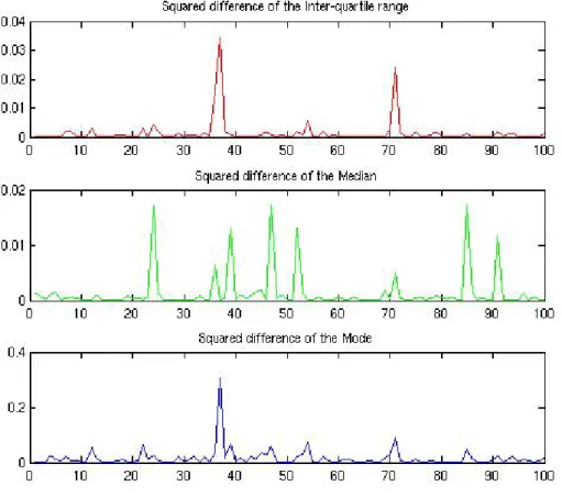
Chart 3: Squared difference between “undisturbed” and “disturbed” empirical statistical indices (Two - lognormal method)

(25)

Chart 4: Squared difference between “undisturbed” and “disturbed” empirical statistical indices (Shimko’s method)

As we can see from Table 3, Chart 3 and Chart 4, Shimko’s method provides an implied density which is less sensitive to “small” pricing errors. There again, it seems that the result above come from the robustness of a linear regression of implied volatility on strike prices. It seems that the optimization procedure in the two-lognormal method is somewhat sensitive to small pricing errors. Thus, as it may seem, Shimko’s non-parametric method is more robust in the case of TASE dollar options. This result is similar to that obtained by Bliss & Panigirtzoglou.

3. Probability Integral Transform

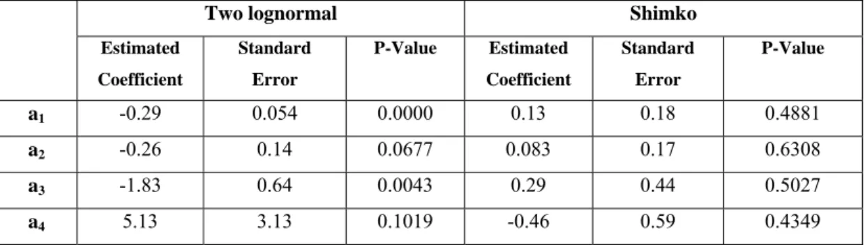
Table 5 presents the results obtained from the GMM procedure that was run for both PIT transformations.

(26)

Table 5: GMM results for the Probability Integral Transform

Two lognormal Shimko

Estimated Coefficient Standard Error P-Value Estimated Coefficient Standard Error P-Value a1 -0.29 0.054 0.0000 0.13 0.18 0.4881 a2 -0.26 0.14 0.0677 0.083 0.17 0.6308 a3 -1.83 0.64 0.0043 0.29 0.44 0.5027 a4 5.13 3.13 0.1019 -0.46 0.59 0.4349

The results for the Probability Integral Transform test suggest that the non-parametric method gives an empirical implied density that is a reasonable forecast of the “true” density. This might be evidence that the two-lognormal assumption is not adequate in modeling the price process of the underlying asset.

4. Results analysis

The obtained results give a significant advantage to Shimko’s method for extracting the implied risk neutral density from option prices. This non-parametric method gives a density for which synthetic option prices better fit observed market prices. It is more robust to pricing errors and in terms of forecast ability it does significantly better job than the two - lognormal method. However, Shimko’s method has a major weakness in comparison to the two-lognormal method. In days where options are traded in a narrow strike range, Shimko’s method generates an implied density that has a worse fit relative to observed option prices. This might also have consequences on its robustness and forecast ability on a given day. This weakness is not surprising, since the strength of Shimko’s method is a function of the goodness of fit of the regression process of implied volatilities on observed strike prices. Thus, given a narrow range of strike prices, the regression of implied volatilities on strikes does not capture the whole smile.

This naturally has an effect on the shape of Shimko’s implied density. Under a narrow range of strikes, the shape of the implied density is such that even a graphical

(27)

interpretation of the implied density is not possible. This is where the parametric approach does a better job than Shimko’s method. Of course, it is possible to fully follow Shimko’s footsteps and graft the tails of a theoretical lognormal density. However, I do not believe that this is adequate given the fact that there is strong evidence against the lognormal assumption in modeling the US dollar/New Israeli Shekel exchange rate.

V. Conclusion

In this research paper, two methods for obtaining implied risk neutral densities from exchange traded FX options were reviewed and compared in term of their ability to: fit between theoretical and observed option prices, to be more robust to pricing errors and to be a reasonable forecast of expectations on future changes in the underlying asset prices.

In general, Shimko's method for obtaining the implied risk neutral densities does a better job in for exchange rate between the U.S dollar and the New Israeli Shekel. The strength of this method comes from being in many ways more empirically sound than the two log – normal. As mentioned previously, methods using the Implied Volatility Smile to obtain a probability density of expected future changes in exchange rate captures better the information embedded in traded option prices.

However, this method has some major weaknesses. The first and most striking weakness is that the data is uninformative about the tails of the distribution, which prevents the calculation of some key statistics such as the mean and standard deviation of the implied density. The second weakness, which relates directly to the first, is that this method performs poorly on days where the range between the minimal and the maximal strike price is small. The narrow range of strike prices (in the context of small number of observations) also influences the degrees of freedom for the curve that fits the implied volatility smile.

Nevertheless, Shimko's implied density usually gives us a more reliable density for forecasting future changes in the exchange rate. Overall, it is also more robust to errors in prices. However, perhaps the robustness of the two – lognormal method can be

(28)

significantly improved by adapting a better optimization method that is used by MATLAB© optimization toolbox. I have tried using the adaptive simulated annealing optimization algorithm19_{. However, this algorithm underperformed and took more time to}

give results20. Note also that the MATLAB optimization toolbox usually performs poorly in comparison to other statistical and mathematical software.

Another direction in improving the parametric method is to assume a different probability law for returns on the exchange rate. Perhaps a more suitable statistical law exists for these returns. Examples of possible candidates are the Generalized Beta of Second Order (GB2) distribution, the g-h distribution, the Weibull, the Generalized Extreme Value (GEV) distribution, and other possible candidates.

Technical Report, 2002, Linkoping Institute of Technology

(29)

Bibliography

Ait – Sahalia, Y. and Lo, A., 'Nonparametric estimation of state-price densities implicit in financial asset prices', Journal of Finance, Vol. 53, 1998, pp. 499-548

Alonzo F. et al., 'Testing the Forecasting Performance of IBEX 35 Option Implied Risk Neutral Densities', Working Paper, 2005, Bank of Spain

Anagnou I. et al., 'The Relation between Implied and Realised Probability Density Functions', Working Paper, 2003, University of Warwick

Bates, D.S, 'The crash of '87: Was it expected? The evidence from options markets',

Journal of Finance, Vol. 46, 1991, pp. 1009-1044

Bahra, B., 'Implied Risk-Neutral Probability Density Functions from Option Prices: Theory and Application', Working Paper, 1997, Bank of England

Black, F. and Scholes, M., 'The pricing of options and corporate liabilities', Journal of Political Economy, Vol. 81, 1973, pp. 637-654

Bliss, R. and Panigirtzoglou, N., 'Testing the Stability of Implied Probability Density Functions', Journal of Banking and Finance, Vol. 26, 2002, pp. 381-422

Breeden, D.T., and Litzenberger, R.H, 'Prices of State-Contingent Claims Implicit in Option Prices', Journal of Business, Vol. 55, 1978, pp. 621-651

Craig B. et al, 'The forecasting performance of German Stock Option Densities', Discussion Paper, 2003, Deutsche Bundesbank

Christoffersen P., and Mazzotta S., 'The Informational Content of Over-the-Counter Currency options', Working Paper, 2004, European Central Bank

Diebold F. X. et al., 'Evaluating Density Forecasts with applications to Financial Risk Management', International Economic Review, Vol. 39, 1998, pp. 863 – 883

Garman M.B., and Kohlhagen S.W., 'Foreign Currency Option Values', Journal of International Money and Finance, Vol. 2, 1983, pp. 231-237

Gemmill G., and Saflekos A., 'How useful are Implied Distributions? Evidence from Stock Index Options', Journal of Derivatives, Vol. 7, 2000, pp. 83 - 98

Gurkaynak R., and Wolfers J., 'Macroeconomic Derivatives: An initial analysis Of Market – Based Macro Forecasts, Uncertainty, and Risk', Working Paper, 2005, NBER Malz A.M., 'Using Option Prices to Estimate Realignment Probabilities in The European Monetary System', Working Paper, 1995, Federal Reserve Bank of New-York

(30)

Moins S., 'Implementation of a simulated annealing algorithm for MATLAB©', Technical Report, 2002, Linkoping Institute of Technology

Rosenblatt M. (1952), 'Remarks on a Multivariate Transformation', Annals of Mathematical Statistics, 23, 470-472.

Shimko D., 'Bounds of Probability', Risk, Vol. 6, 1993, pp. 33-37

Stein R. and Hecht Y., 'Distribution of the Exchange Rate Implicit in Option Prices: Application to TASE', Working Paper, 2003, Bank of Israel

Stein R., 'The Expected Distribution of Exchange Rate: A Non – Parametric implied Density in FX Options (In Hebrew)', Working Paper, 2005, Bank of Israel

Syrdal S.A., 'A study of Implied Risk-Neutral Density Functions in the Norwegian Option Market', Working Paper, 2002, Bank of Norway

(31)

Annex 1: Sunday effects on the Implied Density

For the purpose of demonstrating the effects of non – synchronous trading between the derivative and the underlying market, the Implied Risk Neutral Density will be derived once using the quoted exchange rate and once with the implied from the put – call parity equation exchange rate. I chose Sundays, where non – synchronous trading is most apparent (there is no trade in the underlying market). The dates chosen were the following:

• Sunday February 20th_{, 2005 (quoted exchange rate: 4.3612NIS per 1$, implied}

exchange rate: 4.3167NIS per 1$)

• Sunday January 15th_{, 2006 (quoted exchange rate: 4.6206NIS per 1$, implied}

• Sunday May 7th_{, 2006 (quoted exchange rate: 4.4736NIS per 1$, implied}

An examination of the deviation between the implied and quoted exchange rates on other days of the week suggests that the option on the dollar market is not inefficient.

Effects apparent in the Non – Parametric Method

The charts below of implied densities suggest that the deviation between the implied and quoted spot exchange rate has an effect on the left and right sides of the implied densities. This might bring to unreasonable probabilities for extreme fluctuation in the exchange rate. There is also an effect on the inter quartile range (which is a proxy of volatility) Chart A: Implied non-parametric density on Sunday February 20th, 2005:

(32)

Chart B: Implied non-parametric density on Sunday January 15th, 2006:

(33)

Effects apparent in the Parametric Method

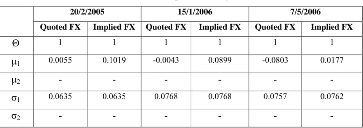
As the following table and charts illustrate, the deviation between the implied and quoted exchange rates has an effect on the location of the obtained implied densities. To be more precise, this deviation affects the mean of the implied density and slightly affects the standard deviation (which is an estimate of implied volatility in this case).

Table A: Parameter estimates of the implied density

20/2/2005 15/1/2006 7/5/2006 Quoted FX Implied FX Quoted FX Implied FX Quoted FX Implied FX

Θ 1 1 1 1 1 1 μ1 0.0055 0.1019 -0.0043 0.0899 -0.0803 0.0177 μ2 - - - - - - σ1 0.0635 0.0635 0.0768 0.0768 0.0757 0.0762 σ2 - - - - - -

(34)

Chart E: Implied parametric density on Sunday January 15th, 2006:

(35)

Annex 2: Rules for extracting the Implied Exchange Rate

In this annex, I will present the rules for extracting the previous implied exchange rate. The rules are the following:

• Bid-Ask Spread: Within a given Bid and Ask quotes we omit options where: 1 , , , − _≥ t i t i t i Ask Ask Bid , where

o Bidi, - is the bid quote of the i'th option at time t

o Askit - is the ask quote of the i'th option at time t

• Moneyness: We omit options that are far from the money such that: 1 . 0 , , ≥ − t i t i t K K S , where

o St ,Ki – The exchange rate and strike price respectively

The implied exchange rate is then calculated as the mean of the most at the money options at each time to maturity21.

Testing techniques and forecasting ability of FX Options Implied Risk Neutral Densities