What can we tell about global auroral-electrojet activity from a single meridional magnetometer chain?

HAL Id: hal-00316231

https://hal.archives-ouvertes.fr/hal-00316231

Submitted on 1 Jan 1996

HAL is a multi-disciplinary open access

archive for the deposit and dissemination of sci-entific research documents, whether they are pub-lished or not. The documents may come from teaching and research institutions in France or abroad, or from public or private research centers.

L’archive ouverte pluridisciplinaire HAL, est destinée au dépôt et à la diffusion de documents scientifiques de niveau recherche, publiés ou non, émanant des établissements d’enseignement et de recherche français ou étrangers, des laboratoires publics ou privés.

What can we tell about global auroral-electrojet activity

from a single meridional magnetometer chain?

K. Kauristie, T. I. Pulkkinen, R. J. Pellinen, H. J. Opgenoorth

To cite this version:

K. Kauristie, T. I. Pulkkinen, R. J. Pellinen, H. J. Opgenoorth. What can we tell about global auroral-electrojet activity from a single meridional magnetometer chain?. Annales Geophysicae, European Geosciences Union, 1996, 14 (11), pp.1177-1185. �hal-00316231�

Ann. Geophysicae 14, 1177—1185 (1996) ( EGS — Springer-Verlag 1996

What can we tell about global auroral-electrojet activity

from a single meridional magnetometer chain?

K. Kauristie1, T. I. Pulkkinen1, R. J. Pellinen1, H. J. Opgenoorth2

1 Finnish Meteorological Institute, Department of Geophysics, Helsinki, Finland 2 Swedish Institute of Space Physics, Uppsala, Sweden

Received: 11 September 1995/Revised: 13 June 1996/Accepted: 25 June 1996

Abstract. The AE indices are generally used for monitor-ing the level of magnetic activity in the auroral oval region. In some cases, however, the oval is either so expanded or contracted that the latitudinal coverage of the AE magnetometer chain is not adequate. Then, a lon-gitudinal chain in the key region would give more in-formation of the real situation, but, of course, only during some limited UT-period. In order to find out the UT coverage of a single meridional chain, we have compared the global A¸ and Aº indices with corresponding local indices determined using data from the meridional part of the EISCAT Magnetometer Cross during the years 1985—1987. A statistical study shows that the local indices are close (within relative error of 0.2) to the global Aº and A¸ during periods 1500—2000 UT (&1730—2230 MLT) and 2130—0130 UT (&0000—0400 MLT), respectively. In the middle of these optimal MLT-sectors the EISCAT Cross sees more than 70% of the cases when the global AE chain records activity. Then, also the correlation be-tween the local and global indices is generally good ('0.7). Thus we conclude that five to six evenly located meridional chains are needed for covering all the UT-periods. On the other hand, already the combination of IMAGE, CANOPUS, and the Greenland chains catches &50% of the substorms. Case-studies show that usually during 2130—1100 UT the A¸ achieved from these chains reproduces the real A¸ with good timing, although it does not follow all transient variations.

1 Introduction

The auroral-electrojet indices (Aº, A¸, and AE, hereafter called the AE indices) were designed in late 1960s by Davis and Sugiura (1966) for routine-type monitoring of the

Correspondence to: K. Kauristie

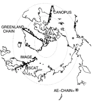
ionospheric currents in the auroral oval region. These indices are based on magnetic recordings of twelve ob-servatories distributed along the auroral oval region (Fig. 1). Aº and A¸ are the upper and lower envelope curves, respectively, of the superposed H-component vari-ations (in intensity, but not in direction) observed at these stations, and AE"Aº!A¸ (Fig. 2). Before the super-position, the measurements are normalized by subtracting base-line values from the data. These base lines are deter-mined for each station and for each month by averaging all H values on the five internationally quiet days. Davis and Sugiura used 2.5-min resolution in their original work, but nowadays AE indices are produced with 1-min resolution.

The ionospheric currents in the oval region are affected both by magnetopause-solar wind interaction processes and by energy release processes in the magnetotail. When energy and particles are transferred from the solar wind to the magnetosphere via dayside reconnection, usually both the eastward and westward auroral electrojets experience a smooth enhancement (directly driven activity). A part of the solar-wind energy and particles is stored into the magnetotail and dissipated later as abrupt bursts to the ionosphere, causing an extra strong westward electrojet (loading-unloading activity) to the midnight sector of the auroral oval (Baker et al., 1984).

Due to their relatively simple definition, the AE indices are easy to relate both to their physical back-ground and to other physical quantities. Aº and A¸ are generally assumed to express the strongest current densities of east-ward (in the evening sector) and westeast-ward (in the morning sector) electrojets, respectively. Electrojet activity, how-ever, is latitudinally limited and thus the AE indices are reliable only if the contributing AE station happens to be at the right latitudes.

During substorms, both directly driven and loading-unloading activity are present in the AE indices. Aº increases smoothly during the substorm growth and ex-pansion phases and decays back to quite-time values during the recovery phase, while A¸ shows more dynamic

Fig. 2. Construction of the AE indices. ºpper

panel: the global AE indices. ¸ower panel: the

local quasi-Aº and A¸ indices Fig. 1. The AE stations and the IMAGE/EISCAT (EISCAT is the

shorter part within the tick marks in the middle of the IMAGE chain), CANOPUS, and Greenland magnetometer chains. The sta-tions used in the case-studies are marked with asterisks. The dotted

lines show the corrected geomagnetic latitudes 60, 70, and 80

behavior, especially during the expansion phase, which typically starts with an abrupt A¸ drop (Fig. 2; Caan et al., 1978; Kamide and Kroehl, 1994).

From the viewpoint of statistical studies the AE indices are superior to other activity indices. In addition to their physically relevant definition, they cover a significant part of the interesting oval region, have adequate time-resolu-tion, are easily available, and long time-series exist. Thus they have been used in many studies concerning, e.g., the solar wind-magnetosphere interaction (Bargatze et al., 1985; Baker et al., 1990; Shan et al., 1991; Takalo et al., 1993) and substorms (Caan et al., 1978; Kamide and Kroehl, 1994; Pellinen et al., 1994; Weimer, 1994; Kauris-tie, 1995).

According to Kamide and Akasofu (1983), the accuracy of the AE indices reduces when magnetic activity de-creases below 250 nT. Then the oval is so contracted that the AE stations cannot monitor it properly. Similarly, during strong activity the oval expands to such low lati-tudes that the AE chain cannot follow the electrojet activ-ity either. Furthermore, during continuously enhanced activity (e.g., steady convection periods), the oval can be much wider than it usually is, also leading to possible misinterpretations of the activity level if only AE indices are used (Sergeev et al., 1996). In such cases a meridional chain is necessary for discriminating spatial effects from real temporal behavior. The longitudinal coverage of a single meridional chain is, however, limited.

Questions like what are the activity level and the longi-tudinal (or UT) coverages of a single chain, or which UT-periods can be covered with the present operating meridional chains, are important now during the ISTP (International Solar Terrestrial Physics) program, as in-formation on the global magnetic activity level is required in a rapid time-scale after the satellite observations (e.g., from WIND, POLAR, GEOTAIL, and INTERBALL). New preliminary oval indices (resembling A¸ index) based on data from some automated stations are already avail-able (see the World Wide Web at http://wdcc1.bnsc.rl. ac.uk/gbdc/auroralovals.html). There are three indices monitoring activity in contracted, standard (at the latit-udes of AE stations), and expanded oval. The coverage of the indices is improved continuously as data from new stations are obtained. In addition to magnetic recordings data from radars and optical instruments are also needed to support the satellite measurements which provide high-resolution data, but suffer from spatial-temporal ambi-guity. The ground-based observations help in placing the in situ observations in a wider context and provide important information of the ionospheric boundary con-ditions.

We compare the global A¸ and Aº (A¸glo and Aºglo) indices with corresponding local quasi-indices (A¸loc and Aºloc) determined using the recordings of the EISCAT Magnetometer Cross in northern Scandinavia and Fin-land. In Sect. 2 we describe the local data set and the parameters used for characterizing the differences between the local and global indices. The optimal UT-periods when the local indices give relevant information of the global activity are defined in Sect. 3. The activity depend-ence of these UT-periods is analyzed as well. In Sect. 4 the common coverage of the EISCAT/IMAGE, Greenland, and CANOPUS chains is studied during two 1-week test periods. Section 5 comprises the conclusions.

2 Data analysis

The local AE indices are based on the recordings of the EISCAT Magnetometer Cross (c.f. Fig. 1; Lu¨hr et al., 1984) during the years 1985—1987. This cross consists of a main meridional chain (five stations) around geographic longitude &23° and two side stations &3° to the west and east of the main chain. The chain covers magnetic latitudes 63°—67° (here the magnetic coordinates are by Baker and Wing, 1989). We had to omit the recordings of KIL (the western-side station) from the analysis because of technical problems during 1985, but fortunately this does not cause any significant limitations to the longitudi-nal coverage of the local indices.

The local AE indices were constructed with exactly the same procedure as the global AE indices. The base-line values were defined for each month using the average H-component values of the five internationally quiet days (H"JX2#½2, where X and ½ are the geographic north and east components of the magnetic field). After subtracting the base lines the H-components of the six stations were superposed and the envelope curves were

used as local Aº or A¸ indices, when positive or negative, respectively (cf. Fig. 2). Located at one fixed longitude, the EISCAT Cross usually gives either Aº or A¸. However, sometimes close to the Harang discontinuity or during quiet periods the upper envelope curve can be positive and the lower curve negative.

The differences between the local and global indices can be characterized by computing the average relative error, E(t), which is defined, e.g., for A¸, as

EAL(t)"A¸glo(t)!A¸loc(t)_A¸glo(t) , (1) where t is the time (with 1-min resolution). A¸glo and A¸loc are negative and thus EAL is negative when the local chain sees stronger activity than the global one (i.e., when A¸loc(A¸glo, but DA¸locD'DA¸gloD). In this case the devi-ation is due to the improvement in the local index when compared to the global one. When the local chain is outside the key-region, DA¸locD&0 and EAL&1. These limit values are valid also for EAU when defined similarly as EAL. When computing the relative errors the pairs of local and global values were categorized according to magnetic activity and binned to 1-h UT bins. The 1-h averages are used for defining the optimal UT-periods when the relative errors are below 0.2, which we consider as a suitable tolerance level for global activity monitoring. Our definition for the relative error does not take into account the periods when A¸glo'0 or Aºglo(0. Such periods, however, are rare and thus not statistically signifi-cant.

In order to estimate the quality of the local indices further, we computed the Pearson correlation coefficients, C(t), between the two data sets:

CAL(t)"+n i/1 (A¸iglo(t)!AM¸glo(t))(A¸iloc(t)!AM¸loc(t)) ]

A

B

+n

i/1 goes over index values recorded at the moment t, and A¸glo(t) and AM¸loc(t) are the mean values at each UT. We computed CAL and CAU for four different activity levels. The data were binned as whole events (where events are the local and global time-series observed during 24-h UT-periods centered at midnight for A¸ and at noon for Aº), not as individual points as in the case of relative errors. The binning was done according to the minimum (A¸) and maximum (Aº) 1-min values of the events.

Press et al. (1992) present a method for estimating the statistical significance of the correlation coefficients. For large data sets (including hundreds of data points) the correlation coefficient can be considered as a random variable with normal distribution. In the null hypothesis the correlation is assumed to be zero (i.e., the mean value of the normal distribution is zero). The probability of achieving at least the observed correlation value is

computed with the complementary error function

SCAL(t)"_Jn2 =: (D_CAL(t)D Jn_)@J2

exp (!u2) du , (3) where n is number of the observations at the considered t. If SCAL(t) is small (below 0.01 is a commonly used limit), the null hypothesis can be rejected and the correlation can be considered as significant. The optimal UT-periods are defined as periods when significant correlation is larger than 0.7.

3 Comparison between the global and local AU-and AL-indices

3.1 How often and how well does the local chain record activity?

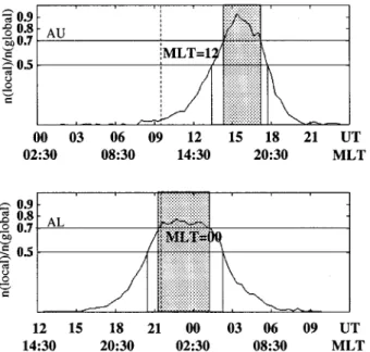
In order to see what are the key regions of the Aº and A¸ activity, we estimated the probability (as a function of UT) of the local chain to record activity when the global chain records it. This was done by comparing 20-min averages of the global and local indices. The local chain was defined to record the global activity when the absolute values of both the averages exceeded 100 nT. Then the number of local activity observations (at each t) was divided by the number of global activity observations. The results are shown in Fig. 3. The EISCAT Cross sees 570% of the Aº activity events during 1430—1700 UT and the A¸ activity events during 2130—0100 UT. During these UT-periods the EISCAT Cross scans the MLT-sectors &1700—1930 and &0000—0330, respectively (hereafter we use only UT-periods from which the approximate MLT-sectors are obtained by adding 2.5 h).

The UT dependence of the relative errors EAL and EAU are shown in Fig. 4. The average relative errors are smallest during 1500—2000 UT (for Aº) and 2130— 0130 UT (for A¸). In these regions the meridional chain gives a representative estimate of the global activity level. To summarize, Figs. 3 and 4 show the time-periods during each day when, one, the probability of observing a distur-bance is high (Fig. 3) and two, the relative error between the locally measured activity and the activity recorded by the global chain in small (Fig. 4).

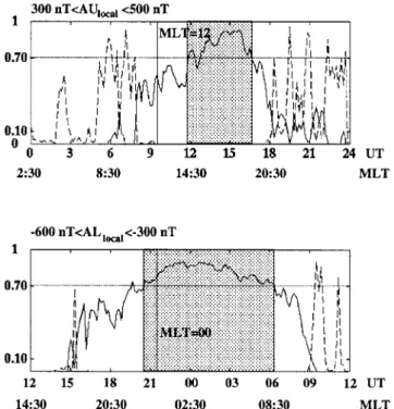
3.2 Dependence on the global and local activity levels The relative errors of Eq. 1 depend also on the intensity of the activation: stronger events are easier to record with a local chain. Figure 5 shows how EAL behaves at different activity levels, when the data have been binned according to local activity. The pairs of data points were categorized into four groups: _{A¸loc(!600 nT, !600 nT4} A¸loc(!300 nT, !300 nT4A¸loc(!100 nT, and A¸loc5!100 nT. The average error curves show the time-periods when the local chain records activity at the given level, and how well in these cases the observed activity describes the global activity. The average error curve for the strongest A¸ activity level shows that the

Fig. 3. Distribution of the local observations of Aº (upper panel) and A¸ (lower panel) activity as functions of UT (or MLT). The gray

shadings mark the UT-periods when the EISCAT Cross catches at

least 70% of the activity events which the AE(12) chain records (for more details, see text)

Fig. 4. UT dependence of the average relative errors between the global and local Aº (upper panel) and A¸ (lower panel). The UT-periods when the error is below 0.2 and below 0 (i.e., the local chain sees stronger activity than the global one) are marked with lighter and darker shadings, respectively

local chain records activity below !600 nT during 1730—0630 UT and then usually also the global chain sees approximately the same activity. In addition, during 1800—0600 UT, EAL is negative and thus the local chain records stronger activity than the global one. At the next two activity levels the local chain records activity during a wider UT-period, but this activity is close to the global index during periods 1800—0400 UT and 2000—0300 UT,

Fig. 5. Activity dependence of the average relative errors between the global and local A¸. The data have been binned according to local activity. The UT-periods when the error is below 0.2 and below 0 (i.e. the local chain sees stronger activity than the global one) are marked with lighter and darker shadings, respectively

respectively. EAL at the lowest activity level shows just that if the local chain cannot see any activity during period 2200—0100 UT then it is really quiet. The narrow time window in this case also shows that small events are easy to miss when not exactly at the correct local time-sector.

Figure 6 presents the activity dependence of EAU (for levels Aºloc(100 nT, 100 nT4Aºloc(300 nT, 300 nT 4Aºloc(500 nT, and Aºloc5500 nT). At the activity level 100 nT4Aºloc(300 nT in almost all UT bins, the local chain records stronger Aº activity than the global chain. However, the number of data points is small in bins other than 1400—1800 UT. At the three other activity

Fig. 6. Activity dependence of the average relative errors between the global and local Aº. The data have been binned according to local activity. The UT-periods when the error is below 0.2 and below 0 (i.e. the local chain sees stronger activity than the global one) are marked with lighter and darker shadings, respectively

levels the local and global Aº are close to each other around 0900—2000 UT, depending strongly on the activity level. The optimal UT-period of Aº does not show as systematic activity dependence as that of A¸, which shortens as the local activity decreases. The wide local time-sectors of negative EAU (especially at the level 100 nT4Aºloc(300 nT) can be partly due to base-line problems, but they also show the latitudinal limitations of the AE chain: the evening-sector eastward electrojet con-tributing to Aº is at lower latitudes than the morning-sector westward electrojet, which contributes to A¸ (Ros-toker and Phan, 1986). Eleven stations of the AE chain are at higher magnetic latitudes than the most southern

station of the EISCAT Cross. These stations do not moni-tor the eastward electrojet as well as the local chain (i.e., EAU(0). On the other hand, during 0600—1200 UT, when the southernmost AE stations Tixie Bay and Cape Wellen (magn. lat. 61°—62°) are in the evening sector (MLT&1800—2400) and contribute to global Aº, EAU is positive.

When the data are binned according to global activity (with the same bins as in Fig. 5), EAL shows nearly similar behavior as in Fig. 4 (being below 0.2 during 2230— 0130 UT at the highest activity level and during 2200— 0200 UT at the other levels). EAU depends on the activity level so that the optimal period shifts to earlier UT hours as the activity increases (being 1430—2030 UT, 1430—1730 UT, 1300—1700 UT, and 1400—1500 UT for the levels Aºglo(100 nT, 100 nT4Aºglo(300 nT, 300 nT4Aºglo(500 nT, and A¸glo5500 nT, respec-tively). The average error curves for the global binning are different (not reproduced here), because in the local bin-ning also the rare data points outside the key regions are very pronounced, while in the global binning they do not have any statistical significance. As a final conclusion from Figs. 4—6, it can be said that when the local chain records significant activity it yields a better representation of the activity than the global index, but on the other hand only when the local chain is in the key regions of Aº and A¸ (c.f. Fig. 3) we can be sure that it catches the major part of the activations.

3.3 The correlation coefficients

The correlation coefficients give a somewhat different view to our problem. The average relative error between two variables can be small even though they behave in a different manner. Figure 7 shows examples of CAU(t) and CAL(t), which are based on data binned according to local activity. The optimal periods defined from CAU(t) and CAL(t) are generally shorter than those in Figs. 5 and 6 (at the highest activity levels), but longer than in Fig. 4. Here again, the same activity levels were used as in the relative error computations. The best correlation is achieved at the highest A¸ activity level, while at the lowest activity levels CAU and CAL did not exceed 0.7 at all. CAL(t) is above 0.7 during periods 2100—0500 UT, 2030—0600 UT, and 2200—0530 UT for the three highest activity levels, respec-tively. For Aº these periods at the second and third activity levels are somewhat shorter: 1200—1630 UT and 1500—1700 UT. In the bin of highest Aº activity level there were too few points for meaningful correlation com-putations. In the other cases the number of data point pairs varied from 50 to 300.

4 Discussion

4.1 Obtaining a global activity index from several, evenly separated chains

With the results just presented we are able to estimate the common coverage of the IMAGE (Lu¨hr, 1994), Greenland

Fig. 7. Correlation (solid line) and an estimate for its statistical significance (dashed line) between the global and local Aº (upper

panel) and A¸ (lower panel) indices. The correlation can be

con-sidered as significant when the dashed line is below 0.01. The gray

shadings show the UT-periods when the correlation is better

than 0.7

(Friis-Christensen et al., 1985), and CANOPUS (Samson et al., 1991) chains (see Fig. 1). These fully automated chains could serve as the primary data sources for provid-ing a quasi-A¸ index only within a few weeks’ time-delay. Assuming that the average error curves would be similar also for the other two chains, the joint coverage of the three chains would be around 14 h (2130—1100 UT).

This result was tested by constructing Aº and A¸ for two 1-week periods (22—28 February and 18—24 March 1991) using the recordings of 17 stations (marked with stars in Fig. 1) from the three chains. Figure 8 shows the constructed A¸ (A¸17) together with the real A¸ index during 5 days from our test periods. The UT-range which, according to our statistical analysis, is beyond the reach of the 17 stations, is marked with the vertical bars. Else-where, the longitudinal distribution of the stations differs from the AE chain (which during the studied periods consisted of 13 stations having essentially the same longi-tudinal distribution as the official AE (12) chain) only with the one AE station between the Greenland and CANOPUS chains. Consequently A¸17 reproduces the real A¸ with good timing (i.e., without significant delays in the abrupt drops), although it does not follow all the variations. The transient differences in the intensity are most probably due to local intensifications which cannot be monitored identically with the two different mag-netometer networks.

Both the average error analysis and the correlation coefficients between A¸loc and A¸glo show that when even in the late morning sector (&0400 MLT), the meridional

Fig. 8. A¸17 (heavy solid line) and the real A¸ index (thin solid line) during 5 days from February—March 1991

chain provides a representative estimate for the global A¸. Especially during the substorm recovery phase the activity concentrates to morning sector (Kamide and Kroehl, 1994). For example, on 19 March around 2000 UT (third panel in Fig. 8), all the chains were in the evening sector, and consequently A¸17 failed to estimate the recovery-phase activity although it took place during the optimal UT-periods. On the other hand, on 21 March during 1200—1500 UT (fourth panel in Fig. 8) an intensive, but relatively short activation took place. Although all the 17 stations were in late morning sector (&0600 MLT), A¸17 gave a good estimate for A¸ both in timing and in inten-sity during the whole substorm.

Thus on average, with the three meridional chains, &50% of the global activity can be covered. With the addition of a few stations in the Russian and/or Alaskan time-sectors would complete the circle to cover almost all local times. In such a case, with the longitudinal coverage of the chains, much more information could be extracted than is today possible with the AE chain. In local studies the chain closest to the key region could be used, e.g., for estimating the location and width of the auroral electrojet. However, we emphasize that applying the error curve of

Fig. 4 to Greenland or CANOPUS chains gives only an estimate of the real error curve which can show some differences in behavior. Furthermore, the IMAGE chain is longer (covering magnetic latitudes &57°—76°) than the former EISCAT chain. Thus the new chain has a better activity coverage, but perhaps also slightly widened UT coverage, than the old chain.

4.2 Improving the predictions with a linear filtering method?

We tried to improve the predictions of global activity from the local measurements by computing a linear filter be-tween the local and global A¸ indices. The goal was to find a filter which gives A¸glo when only A¸loc is known, and the meridional chain is slightly outside its optimal MLT-region. A linear filter predicts A¸glo at the given time t using A¸loc values preceding and following that time, i.e., A¸glo(ti)"+d2

k/~d1akA¸loc(ti`k)#E(ti), where

ak are the filter coefficients, ti is the considered movement (ith time-step from the beginning of the optimal UT-period), and d1 and d2 are parameters defining the number of preceding and following local values taken into account in the prediction. E(ti) is the error between the predicted A¸glo(ti) and the real A¸glo(ti). The coefficients ak can be defined by minimizing the total sum (over all times and events) of the squared errors.

We tested the linear prediction method with 5-min average values of the A¸ events occurring at 2000— 0400 UT. We concentrated on events where the minimum local A¸ value occurred between 0130 and 0400 UT. The local values 50 min before and 75 min after the considered moment were taken into account in the prediction (i.e., d1"10 and d2"15). The main difficulty was to find suitable criteria for categorizing the events. If the filter is defined using a group of very different events, all the other coefficients except that for k"0 smear out. Activity bin-ning according to the local median values appeared to produce the most homogeneous subgroups for this pur-pose (two groups: medians !100—!30 nT and medians below !100 nT). The total amount of events was 52, 26 of which were used for defining the filter and 26 for testing it. In 17 cases of the 26 test events the predicted curve gives somewhat better estimate for A¸glo than A¸loc during 0100—0300 UT. Improved predictions were more com-mon in the lower activity bin (11 of 15 cases) than in the higher activity bin (6 of 11 cases).

Figure 9 shows one of the best examples of the achieved predictions. Although in this case the intensity of the predicted A¸glo is close to the real A¸glo, generally the linear filtering did not improve A¸loc values significantly. Our poor success can be partly due to the unfavorable distribution of the AE stations. For the CANOPUS chain the predictions could be better, because there the nearby AE stations are suitably located for this purpose (Poste-de-la-Baleine and Yellowknife, &30° to the east and west, respectively), while the nearby stations of EISCAT Cross are either too close (Abisko, 4° to the west) or too far (Dixon Island, 49° to the east).

Fig. 9. An example on predicting the A¸ index. The predicted curve has been obtained from the local A¸ indices by linear filtering

Fig. 10. Correlation between the global A¸ and local AE when maximum 1-min local AE'500 nT. The gray shadings show the UT-periods when the correlation is better than 0.7

4.3 Correlation between the local AE and the global AE: possible evidence of eastward-electrojet enhancement during substorms

Figure 10 shows the correlation (computed using 136 pairs of data points at each UT-moment) between the AEloc and A¸glo when maximum 1-min AEloc'500 nT. During 1430—1700 UT, AEloc&Aºloc (because then A¸loc&0 and AºlocO0, c.f. Fig. 3) and during 2130—0100 UT, AEloc&DA¸locD(Aºloc&0 and A¸locO0, c.f. Fig. 3). Around both these periods the correlation is clearly higher than elsewhere. For the nightside this is not surprising, but according to Fig. 10 the Aº activity in the MLT sector &1430—1930 is closely related to the A¸glo activity, too. If a significant part of the A¸glo activity is assumed to be due to loading-unloading processes, our result suggests that also Aº variations correlate well with substorm activity. This could be due to the so-called eastward explosive electrojets. Grafe (1994) shows exam-ples where enhancements of the eastward electrojet are accompanied by enhanced electron precipitation and Pi2 pulsations, i.e., phenomena which are usually related to the substorm current wedge in the midnight sector.

The explosive eastward electrojets are usually more dynamic and at lower latitudes than the convection-type electrojets (Grafe, 1994), and thus the EISCAT Cross (when in the right position) monitors them better than the AE chain. In our analysis, the most active Aº region shifts to earlier MLT values when activity level is increasing. Combining this information with the schematic Fig. 10 of Grafe (not shown here) suggests that the possible observa-tions of explosive eastward electrojets concentrate to the events of our highest activity bin.

5 Conclusions

We have made comparisons between the global Aº and A¸ indices and corresponding quasi-indices determined from the recordings of the meridional part of the EISCAT Magnetometer Cross. Our statistical studies reveal that the main part of the local Aº and A¸ values are achieved when the meridional chain scans the MLT-sectors 1700—1930 and 0000—0330, respectively. Then the local chain catches 70% of the cases when the global chain sees activity. In MLT-sectors 1730—2230 (for Aº ) and 0000—0400 (for A¸), the strength of the observed local activity is on average more than 80% of the simultaneous global activity (c.f. Fig. 11), but especially in the middle of these optimal MLT-sectors the local indices usually show stronger activity than the global ones. Thus the meridi-onal chain monitors better the activity in the expanding oval than a single AE station.

The optimal MLT-sector of A¸ activity does not show any significant dependence on global activity level (but stays around &0030—0430 MLT), while that of Aº activ-ity shifts to later MLT values as the activactiv-ity decreases (1630—1730 MLT when _{Aºglo'500 nT and 1700—} 2300 MLT when Aºglo(100 nT). Binning according to local activity shows that in those rare cases when strong activity outside the optimal MLT-sectors is observed, it is usually stronger than in the global indices.

In the optimal MLT-sectors the correlation coefficient between the local and global indices is generally higher than 0.7. The correlation coefficient is at this level also for one or two MLT hours before (for Aº) or after (for A¸) the optimal periods. Thus in these sectors the local indices follow the behavior of the global indices, although their variations are not strong.

We tested the possibility of improving the longitudinal coverage of the EISCAT Cross by defining a linear filter between A¸glo and A¸loc. Such a filter could be used for predicting A¸glo when only A¸loc is available. However, due to the great variability in the location and spatial scales of substorm activity, finding representative filters was difficult. Thus no significant improvement in the UT coverage was achieved with this method.

Fig. 11. The MLT regions (marked with gray shadings) where the local EISCAT chain gives a good estimate for the global activity (i.e. when EAU(0.2 or EAL(0.2)

The presented results lead us to conclude that five to six evenly located meridional chains are needed for continu-ous monitoring of the magnetospheric substorm activity. In an ideal situation we could achieve improved AE indi-ces like in the study by Kamide et al. (1982), who use AE70 including data from six magnetometer chains. Never-theless, the combination of the IMAGE, CANOPUS and the Greenland chains catches a significant part of the substorms, as these stations together cover the UT-peri-ods from 2130 to 1100. Case-studies show that the A¸ constructed using these chains generally reproduces the real A¸ without any significant timing delays. According to the results presented in Fig. 5, a single magnetometer chain records over-300-nT activations occurring within $5 h of the magnetic midnight. Thus, data from a single chain can provide information about active events for a significant portion of time.

Acknowledgements. The official AE data were kindly provided by

the WDC-C2 in Kyoto and the preliminary indices for the period February-March 1991 by the Working Group on Ground-Based Observations for INTERBALL. EISCAT Magnetometer Cross was a joint German-Finnish project conducted by the Technical Univer-sity of Braunschweig. The CANOPUS magnetometer data were provided by Terry Hughes and the CANOPUS instrument array was constructed and is maintained and operated by the Canadian Space Agency. We thank also Don Wallis (Herzberg Institute for Astrophysics, National Research Council, Canada) for experienced guidance in the data analysis. The data of the Greenland mag-netometer network were received from Susanne Vennerstro¨m (So-lar-Terrestrial Physics Division, Danish Meteorological Institute). We are obliged to Ari Viljanen for providing the program package for the analysis of the EISCAT Cross data. The work of K. K. was supported by the Academy of Finland.

Topical Editor K.-H. Glaßmeier thanks Y. Kamide and two other referees for their help in evaluating this paper.

References

Baker, K. B., and S. Wing, A new magnetic coordinate system for conjugate studies at high latitudes, J. Geophys. Res., 94, 9139—9143, 1989.

Baker, D. N., S.-I. Akasofu, W. Baumjohann, J. W. Bieber, D. H. Fairfield, E. W. Hones, Jr., B. Mauk, R. L. McPherron, and T. E. Moore, Substorms in the magnetosphere, in Solar ¹errestrial

Physics — Present and Future, NASA Publ., 1120, Chapter 8,

1984.

Baker, D. N., A. J. Klimas, R. L. McPherron, and J. Bu~ chner, The evolution from weak to strong geomagnetic activity: an intrep-retation in terms of deterministic chaos, Geophys. Res. ¸ett., 17, 41—44, 1990.

Bargatze, L. F., D. N. Baker, R. L. McPherron, and E. W. Hones, Jr., Magnetospheric impulse response for many levels of geomag-netic activity, J. Geophys. Res., 90, 6387—6394, 1985.

Caan, M. N., R. L. McPherron, and C. T. Russell, The statistical magnetic signature of magnetospheric substorms, Planet. Space

Sci., 26, 269—279, 1978.

Davis, T. N., and M. Sugiura, Auroral electrojet activity index AE and its universal time variations, J. Geophys. Res., 71, 785—801, 1966.

Friis-Christensen, E., Y. Kamide, A. D. Richmond, and S. Mat-shushita, Interplanetary magnetic field control of high-latitude electric fields and currents determined from Greenland mag-netometer data, J. Geophys. Res., 90, 1325—1338, 1985. Grafe, A., Freja electron precipitation as a hint for an explosive

development of the eastward electrojet, in Proceedings of the

Second International Conference on Substorms, Fairbanks,

Alaska, 7—11 March 1994, 391—398, 1994.

Kamide, Y., and S.-I. Akasofu, Notes on the auroral electrojet indices, Rev. Geophys. Space Phys., 21, 1647—1656, 1983. Kamide, Y., and H. W. Kroehl, Auroral electrojet activity during

isolated substorms at different local times: a statistical study,

Geophys. Res. ¸ett., 20, 389—392, 1994.

Kamide, Y., B.-H. Ahn, S.-I. Akasofu, W. Baumjohann, E. Friis-Christensen, H. W. Kroehl, H. Maurer, A. D. Richmond, G. Rostoker, R. W. Spiro, J. K. Walker, and A. N. Zeltsev, Global distribution of ionospheric and field-aligned currents during substorms as determined from six IMS meridian chains of magnetometers: initial results, J. Geophys. Res., 87, 8228—8240, 1982.

Kauristie, K., Statistical fits for auroral oval boundaries during the substorm sequence, J. Geophys. Res., 100, 21885—21895, 1995. Lu~ hr, H., The IMAGE Magnetometer Network, S¹EP Interntional,

4, 4—6, 1994.

Lu~ hr, H., S. Thu~rey, and N. Klo~cker, The EISCAT-magnetometer cross, technical aspects — First results, Geophys. Surv., 6, 305—315, 1984.

Pellinen, R., T. Pulkkinen, and K. Kauristie, Have we learned enough about auroral substorm morphology during the past 30 Years?, in Proceedings of the Second International Conference on

Sub-storms, Fairbanks, Alaska, 7—11 March 1994, 43—48, 1994.

Press, W. H., S. A. Teukolsky, W. T. Vetterling, and B. P. Flannery,

Numerical Recipes in C, ¹he Art of Scientific Computing, Second

Edition, Cambridge University Press, Cambridge, 1992. Rostoker, G., and T. D. Phan, Variation of auroral electrojet spatial

location as a function of the level of magnetospheric acitivity, J.

Geophys. Res., 91, 1716—1722, 1986.

Samson, J. C., T. J. Hughes, F. Creutzberg, D. D. Wallis, R. A. Greenwald, and J. M. Ruohoniemi, Observations of a detached discrete arc in association with field line resonances, J. Geophys.

Res., 96, 15683—15695, 1991.

Sergeev, V. A., R. J. Pellinen, and T. I. Pulkkinen, Steady magneto-spheric convection: a review of recent results, Space Sci. Rev., 75, 551—604, 1996.

Shan, L.-H., P. Hansen, C. K. Goertz, and R. A. Smith, Chaotic appearance of the AE index, Geophys. Res. ¸ett., 18, 147—150, 1991.

Takalo, J., J. Timonen, and H. Koskinen, Correlation dimension and affinity of AE data and bicolored noise, Geophys. Res. ¸ett., 20, 1527—1530, 1993.

Weimer, D. R., Substorm time constants, J. Geophys. Res., 91, 11005—1994.