Publisher’s version / Version de l'éditeur:
The 2010 International Joint Conference on Neural Networks (IJCNN), pp. 1-8,
2010-07-23
READ THESE TERMS AND CONDITIONS CAREFULLY BEFORE USING THIS WEBSITE. https://nrc-publications.canada.ca/eng/copyright
Vous avez des questions? Nous pouvons vous aider. Pour communiquer directement avec un auteur, consultez la première page de la revue dans laquelle son article a été publié afin de trouver ses coordonnées. Si vous n’arrivez pas à les repérer, communiquez avec nous à [email protected].
Questions? Contact the NRC Publications Archive team at
[email protected]. If you wish to email the authors directly, please see the first page of the publication for their contact information.
NRC Publications Archive
Archives des publications du CNRC
This publication could be one of several versions: author’s original, accepted manuscript or the publisher’s version. / La version de cette publication peut être l’une des suivantes : la version prépublication de l’auteur, la version acceptée du manuscrit ou la version de l’éditeur.
For the publisher’s version, please access the DOI link below./ Pour consulter la version de l’éditeur, utilisez le lien DOI ci-dessous.
https://doi.org/10.1109/IJCNN.2010.5596455
Access and use of this website and the material on it are subject to the Terms and Conditions set forth at
Central England Temperatures and Solar Activity : A Computational
Intelligence Approach
Valdés, Julio J.; Pou, Antonio
https://publications-cnrc.canada.ca/fra/droits
L’accès à ce site Web et l’utilisation de son contenu sont assujettis aux conditions présentées dans le site LISEZ CES CONDITIONS ATTENTIVEMENT AVANT D’UTILISER CE SITE WEB.
NRC Publications Record / Notice d'Archives des publications de CNRC:
https://nrc-publications.canada.ca/eng/view/object/?id=0bd3b1bb-2ce2-4afc-9e7e-47569ba8a92b https://publications-cnrc.canada.ca/fra/voir/objet/?id=0bd3b1bb-2ce2-4afc-9e7e-47569ba8a92bCentral England Temperatures and Solar Activity: A
Computational Intelligence Approach.
Julio J. Vald´es Senior Member, IEEE, and Antonio Pou
Abstract— Two Computational Intelligence techniques,
neu-ral networks-based Multivariate Time Series Model Mining (MVTSMM) and Genetic Programming (GP), have been used to explore the possible relationship between solar activity and temperatures in Central England for the 1721 to 1967 period. Data driven analysis of multivariate, heterogeneous and incomplete time series are used in order to understand the extreme complexity of the climate machinery and to detect the possible relative contribution of influencing processes, like the Sun, whose decadal and centennial role in the climate is still debated.
Experiments were carried out using each one of these techniques and their combination. Time-lag spectra obtained by means of MVTSMM seems to indicate time stamps of some of the relevant Earth-climate and solar variations on the temperature record. The equations provided by GP ap-proximated analytically the relative contribution of particular solar activity time-lags. These preliminary results, even if they still are insufficient to support or discredit possible physical mechanisms, are interesting and encouraging to explore more in that direction.
I. INTRODUCTION
Humans have always tried to find ways to forecast the whims of weather and climate. When sunspot observations became well established, it was natural to look for solar causes. W. Herschel, in 1801, was the first to spot the relationship and publish it [6]. Since then, a large number of scientists have refined the search. The Sun is, no doubt, the source of the Earth’s climate but it acts through a complex network of intermediate mechanisms, which make the finding of simple relationships extremely difficult. Today, since the arrival of satellites, there is a fair knowledge of climate the world over, but it is still difficult to understand the precise role of contributors such as the oceans and the Sun itself.
In the past, the only readily available measurement of the Sun’s activity was counting the variable number of spots which appear on its surface, something that could only be reliably done after Galileo in 1613. During 1843 H. Schwabe observed the evolution of sunspots and suggested the presence of the 11 year cycle bearing his name. Five years later, J. R. Wolf devised the daily index of sunspots activity which remains the main system in use today. At the turn of the 20-th Century, E. W. Maunder discovered a period -from 1645 to 1715- with very low sunspot activity -the Maunder
Julio J. Vald´es is with the National Research Council Canada, Institute for Information Technology, 1200 Montreal Rd. Bldg M50, Ottawa, ON K1A 0R6, Canada (phone: 1-613-993-0887; fax: 1-613-993-0215; email: [email protected]).
Antonio Pou is with the Department of Ecology, Faculty of Sciences, Au-tonomous University of Madrid, 28049-Madrid, Spain (phone: (34)(91)497-8194; fax: (34)(91)497-8001; email: [email protected]).
Minimum. In Europe, by the end of the medieval times, winter temperatures dropped down so much that, in 1939, Matthes coined for that period the rather informal term of ”Little Ice Age”. This period, whose universality is under ongoing discussion, has been repeatedly put in relationship with the Maunder Minimum, establishing the basis for a large research effort on the solar-climate link.
However, there are a number of difficulties: the scarcity and reliability of past climate data (many are just proxies), the difficult reconstruction of long sunspots records, the assumption of a direct relationship with sunspots (but they are also a proxy of the Sun’s activity), and the difficulty of establishing clear cut First-Principles approaches. So, it is not surprising that most climate simulation models avoid the inclusion of external forcing mechanisms and instead put the emphasis on well known intrinsic climate processes Meanwhile, solar physicists have been pointing to the extraordinary activity of magnetic solar ejections for the last half century. Some even say the activity is without precedent in the last ten thousand years [31] [24], but others disagree [22]. The current accepted knowledge about the present climate change implies a major role of the anthropogenic activities [8] while also acknowledging the presence of natural causes, with the Sun leading them.
New research is now focusing on first principles expla-nations for external forcing mechanisms, as they not only may be of relevance to the future of climate investigation but already are of the highest importance for satellites, space exploration and many Earth based systems. Two main and complementary lines of research seem promising: the electric circuitry of the ionosphere-atmosphere-Earth’s surface sys-tem [26] and its modulation via cosmic ray activity [25], both affected by the solar activity and both affecting the processes of cloud formation and hence all the climatic system as a whole. But, apart from theoretical considerations, an important issue is to try to extract more information from the available data.
The maximum common length of monthly climatic and solar data available reaches back to 1659, but probably only yearly aggregated values can be used with some confidence [19]. Computational intelligence techniques have been ex-tensively applied to the analysis of both Earth’s temperature and Solar Sunspots data. Preferred techniques have been neural networks ([32], [9], [18], [33], [16], [17] and many others), but most studies analyze these data separately (with some exceptions like [34] and [14]). Other computational intelligence methods like genetic programming (GP) were first introduced in [30]. The case of genetic programming
is interesting because it produces models in the form of analytical functions, which are very familiar to experts from climatological and astronomic communities.
This paper explores the use of two computational in-telligence techniques: neural networks-based time series model mining and model discovery of analytic functions (via genetic programming); for mining relationships between measured temperatures on earth and solar activity. These techniques are applied independently and then combined, complementing each other. This is a promising approach for determining potential relationships among several time-series of different complex processes. The neural networks-based time series model mining (MVTSMM) focuses on extracting information about the inner structure of the series, whereas in genetic programming explicit analytic functions are constructed as function approximations describing the data. It could very helpful to determine and quantify the relative contribution of natural and anthropogenic causes behind present climatic change. Hopefully it would be done.
II. DATA
The longest available instrumental temperature record is the one compiled by Manley [15] for central England, which dates backs to 1772 for mean daily data and to 1659 for mean monthly data. Maximum and minimum daily data are also available, beginning in 1878. The record is built from inland representative stations, a roughly triangular area enclosed by Bristol, Lancashire and London, most of them resembling the records from stations of the rural lowlands areas (100-200 m in height) of Staffordshire, Shropshire and North Warwickshire. Extreme care was put by Manley on location; avoiding frost-hollows or windswept ridges, trying to find ”the most probable mean temperature” of a group of well-run stations of the midlands countries, and making adjustments to century old monthly means in order to bring them to modern standards. Since 1974 the data have been adjusted to allow for urban warming. The uncertainty had been assessed since 1878 [19]. Accordingly, this study focusses on the analysis of mean annual time series instead of monthly means. This choice takes into account the possible delays in climate response to solar activity and the intrinsic difficulties in handling larger amounts of data within the present analytical approach.
The Central England Temperature (CET) data are made available by the British Atmospheric Data Center. The CET 1721-1967 record of mean yearly temperatures is shown in Fig.1 (top). These temperature data have been analyzed in relationship to the solar activity as expressed by the Group Sunspot Numbers (GSN) during the same period of time, Fig.1 (bottom). The sunspots index introduced by Wolf in 1848 is a combination of counting sunspots groups and individual spots. He made a reconstruction of the series till 1700, using historical observations. Today his index, which is often called the Zurich Sunspot Numbers, is published daily by the Sunspot Index Data Center in Belgium. A new index, the Group Sunspots Numbers, has recently been introduced [7],[3] based solely on sunspot groups, allowing more precise
reconstructions of historic conditions while extending the records back to 1610. From 1848 on, both indexes are nearly identical. This paper uses GSN.
III. MULTIVARIATETIMESERIESMODELMINING
The purpose of model mining in complex data coming from heterogeneous, multivariate, time varying processes [27], [28], [29] is to discover dependency models. A model expresses the relationship between values of a previously selected time series (the target), and a subset of the past values of the entire set of series. Different classes of func-tional models may be considered, in particular, a generalized non-linear auto-regressive (AR) model
𝑆𝑇(𝑡) =
F
⎛ ⎜ ⎜ ⎝ 𝑆1(𝑡 − 𝜏1,1), ⋅ ⋅ ⋅ , 𝑆1(𝑡 − 𝜏1,𝑝1), 𝑆2(𝑡 − 𝜏2,1), ⋅ ⋅ ⋅ , 𝑆2(𝑡 − 𝜏2,𝑝2), . . . 𝑆𝑛(𝑡 − 𝜏𝑛,1), ⋅ ⋅ ⋅ , 𝑆𝑛(𝑡 − 𝜏𝑛,𝑝𝑛) ⎞ ⎟ ⎟ ⎠ (1)where 𝑆𝑇(𝑡) is the target signal at time 𝑡, 𝑆𝑖 is the 𝑖-th time series,𝑛 is the total number of signals, 𝑝𝑖is the number of time lag terms from signal𝑖 influencing 𝑆𝑇(𝑡), 𝜏𝑖,𝑘 is the 𝑘-th lag term corresponding to signal 𝑖 (𝑘 ∈ [1, 𝑝𝑖]), and
F
is the unknown function describing the process.The classical approaches in time series mostly consider univariate, homogeneous (real-valued) time series without missing values [2], [23], [21]. Conventional multivariate approaches are complex and have difficulties in handling heterogeneity, imprecision and incompleteness. A hybrid soft-computing algorithm for these kinds of problems using heterogeneous neural networks and genetic algorithms was introduced in [27], in the spirit of [20]. It requires the simultaneous determination of: (i) the number of required lags for each series, (ii) the particular lags within each series carrying the dependency information, and (iii) the prediction function. A requirement on function
F
is to minimize a suitable prediction error measure. The Multivariate Time Series Model Mining procedure (MVTSMM) is based on: (a) exploration of a subset of the model space with a genetic algorithm, and (b) use of a similarity-based neuro-fuzzy system representation for the unknown prediction functionF
. The process implies a search in the space of neuro-fuzzy networks (Fig.2). This approach is usually applied on a sliding time-window so that an exploration of the structure of the multivariate series can be made, using the mined models as indicator of internal changes within the process. One way of describing the results is to compute the weighted lag importance function, whose general form isℒ𝑤(𝑡, 𝜏 𝑝,𝑞) = ∑𝑐𝑎𝑟𝑑( ˆℳ) 𝑖=1 𝜇(𝜏𝑝,𝑞, ˆℳ𝑖(𝑡)) ⋅ 𝑓 ( ˆℳ𝑖(𝑡)) ∑𝑐𝑎𝑟𝑑( ˆℳ) 𝑖=1 𝑓 ( ˆℳ𝑖)(𝑡) (2) where ˆℳ is the set of discovered models for a given window, 𝑐𝑎𝑟𝑑( ˆℳ) is its cardinality, ˆℳ𝑖(𝑡) ∈ ˆℳ is the 𝑖-th model found at time 𝑡, 𝜇(𝜏𝑝,𝑞, ˆℳ𝑖(𝑡)) is the boolean membership function of lag 𝜏𝑝,𝑞 ( from Eq.1 ) with respect to ℳˆ𝑖(𝑡), and 𝑓 ( ˆℳ𝑖(𝑡)) is a strictly positive model quality measure (fitness) on ˆℳ.
Fig. 1. Central England Temperatures (CET) and Group Sunspot Numbers (GSN) in the period1721 − 1967. The vertical line at 1888 indicates the division between the training and validation sets (75% for training and 25% for validation).
Fig. 2. Multivariate Time Series Model Miner System (MVTSMM). The arc (left) is a parallel genetic algorithm evolving populations of similarity-based hybrid neural networks. The binary strings encode dependency patterns for the target signal. For each, a hybrid neural network is constructed and trained with a fast algorithm. The network represents the prediction function, and is applied to an independent validation set. The best models are collected.
IV. GENETICPROGRAMMING
Analytic functions are among the most important building blocks for modeling, and are a classical way of expressing knowledge, which has a long history of usage in science. From a data mining perspective, direct discovery of general analytic functions poses enormous challenges because of the (in principle) infinite size of the search space.
Within computational intelligence, genetic programming techniques aim at evolving computer programs, which ulti-mately are functions. Genetic Programming (GP) introduced in [10] and further elaborated in [11], [12] and [13], is an extension of the Genetic Algorithm. GP starts with a set of randomly created computer programs. This initial population goes through a domain-independent breeding process over a series of generations. It employs the Darwinian principle of survival of the fittest with operations similar to those oc-curring naturally, like recombination of entities (crossover), occasional mutation, duplication and gene deletion. A
com-puter program is understood as an entity that receives inputs, performs computations which transform these inputs and produces some output in a finite amount of time. The op-erations include arithmetic computation (possibly involving many other functions), conditionals, iterations, recursions, code reuse and other kinds of information processing or-ganized into a hierarchy. GP combines the expressive high level symbolic representations of computer programs with the search efficiency of the genetic algorithm. For a given problem, this process often results in a computer program which solves it exactly, or if not, at least provides a fairly good approximation.
There are several approaches to GP leading to a plethora of variants (and implementations) and a discussion about their relative merits, drawbacks and properties is beyond the scope of this paper. One of these GP techniques is the Gene Expression Programming (GEP) [4], [5]. GEP individuals are nonlinear entities of different sizes and shapes (expression trees) encoded as strings of fixed length. For the interplay of the GEP chromosomes and the expression trees (ET), GEP uses an unambiguous translation system to transfer the language of chromosomes into the language of expression trees and vise versa. The structural organization of GEP chromosomes allows a functional genotype/phenotype relationship, as any modification made in the genome always results in a syntactically correct ET or program. The set of genetic operators applied to GEP chromosomes always produces valid ETs. The chromosomes in GEP itself are composed of genes structurally organized in a head and a tail [4]. The head contains symbols that represent both functions (elements from a function set F) and terminals (elements from a terminal set T), whereas the tail contains only terminals. Therefore, two different alphabets occur at different regions within a gene. For each problem, the length of the headℎ is chosen, whereas the length of the tail 𝑡 is a function ofℎ, and the number of arguments of the function with the largest arity. The length of the tail is evaluated given by 𝑡 = ℎ(𝑛 − 1) + 1. As an evolutionary algorithm GEP
defines its own set of crossover, mutation and other operators [5].
V. EXPERIMENTALSETTINGS
The length of the CET and GSN data in the 1721-1967 period is 247 years and from these samples training and validation matrices were constructed using 25 predictor variables from both. Let 𝐶𝐸𝑇 (𝑡) be the observed value of CET at time 𝑡; accordingly, the set of predictor variables was formed as the following lagged variables: 𝐺𝑆𝑁 (𝑡 − 25), 𝐺𝑆𝑁 (𝑡−24), ⋅ ⋅ ⋅ , 𝐺𝑆𝑁 (𝑡−1), 𝐶𝐸𝑇 (𝑡−25), 𝐶𝐸𝑇 (𝑡− 24), ⋅ ⋅ ⋅ , 𝐶𝐸𝑇 (𝑡 − 1), thus making a total of 50 predictor variables. In all experiments the training set contained 75% of the data whereas the remaining 25% was put aside for validation. Accordingly, the number of training samples was 167 and the number of validation samples 55.
Different types of experiments were made with the above described data:
Exp.1 Model mining via Genetic Programming using the training and validation matrices with the50 original predictor variables.
Exp.2 MVTSMM exploration of the bivariate GSN-CET series:
a using a single observation window cover-ing the entire length of the series, in order to characterize the process as a whole. b sliding a window of smaller length (101
sampling points), in order to explore the finer structure of the process and detect potential model changes over time. For both Exp.2.a and Exp.2.b suites, the lag importance function (Eq.2) was com-puted. In the case of Exp.2.a, a subset of more relevant predictor variables (time lags) were derived.
Exp.3 Model mining via Genetic Programming using training and validation matrices containing only the selected lags from Exp.2.a as predictor variables. All genetic programming experiments were conducted us-ing the GEP technique described in Section.VI-A with a fixed Function set given by {+, −, ∗, 𝑥𝑦, 𝑒𝑥, 𝑙𝑛(𝑥)}. Experiments of the Exp.1 suite used the parameters shown in Table.I. In total the Exp.1 suite contained 62, 208 evolutionary compu-tation runs.
In the MVTSMM exploration a group of parameters define on one hand the kind of genetic algorithm to use, and on the other hand, the specificities of the similarity-based neural network model to use [27], [28]. Among these parameters, the type of similarity function, the number of responsive neurons in the hidden layer, etc. play an important role. This is because the network is designed to produce only a coarse estimate of the target, with a training scheme that doesn’t iterate over the training set and therefore is extremely fast. This is a requirement imposed by the fact that the genetic algorithm evolves populations of such networks. The similarity functions used in the neuron model at the hidden
TABLE I
EXPERIMENTAL SETTINGS FOR THEGENETICPROGRAMMING RUNS CORRESPONDING TO THEEXP.1SUITE(62, 208RUNS).
Parameter values seed {3292, 19257, 27576} generations {200, 1000, 2000} population size {200, 300, 400} inversion prob {0.1, 0.2} mutation prob {0.044, 0.06} num genes {5, 8, 12} gene head size {8, 12, 15} is transposition {0.1, 0.2} ris transposition {0.1, 0.2} one point recomb {0.3, 0.5} two point recomb {0.3, 0.5} gene recomb {0.1, 0.2} gene transposition {0.1 , 0.2 }
layer are derived from well known distance functions by the transformation 𝑠 = 1/(1 + 𝑑), where 𝑠 is a similarity and 𝑑 is a distance function. The experimental settings used for the MVTSMM runs corresponding to the Exp.2.a suite are shown in Table.II. In this case, the entire signal is covered by a single exploration window characterizing the process as a whole and it provides a one-dimensional lag importance function (Eq.2).
TABLE II
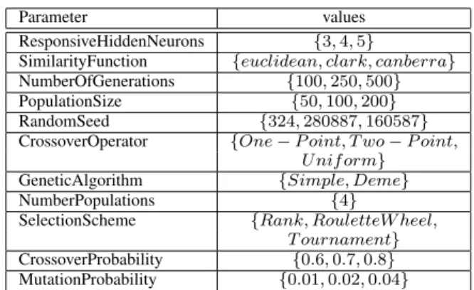
EXPERIMENTAL SETTINGS FOR THEMVTSMMRUNS CORRESPONDING TO THEEXP.2.A SUITE. Parameter values ResponsiveHiddenNeurons {3, 4, 5} SimilarityFunction {𝑒𝑢𝑐𝑙𝑖𝑑𝑒𝑎𝑛, 𝑐𝑙𝑎𝑟𝑘, 𝑐𝑎𝑛𝑏𝑒𝑟𝑟𝑎} NumberOfGenerations {100, 250, 500} PopulationSize {50, 100, 200} RandomSeed {324, 280887, 160587} CrossoverOperator {𝑂𝑛𝑒 − 𝑃 𝑜𝑖𝑛𝑡, 𝑇 𝑤𝑜 − 𝑃 𝑜𝑖𝑛𝑡, 𝑈 𝑛𝑖𝑓 𝑜𝑟𝑚} GeneticAlgorithm {𝑆𝑖𝑚𝑝𝑙𝑒, 𝐷𝑒𝑚𝑒} NumberPopulations {4} SelectionScheme {𝑅𝑎𝑛𝑘, 𝑅𝑜𝑢𝑙𝑒𝑡𝑡𝑒𝑊 ℎ𝑒𝑒𝑙, 𝑇 𝑜𝑢𝑟𝑛𝑎𝑚𝑒𝑛𝑡} CrossoverProbability {0.6, 0.7, 0.8} MutationProbability {0.01, 0.02, 0.04}
With the purpose of exploring the inner structure of the time varying process, a window of length101 (less than one half of that of the GSN and CET records), was slid along the series. Such a window length (101) is a compromise between a large window in which there are enough training and validation samples and a small enough that enables the detection of changes in time. The experimental settings used for the MVTSMM runs corresponding to the Exp.2.b suite are shown in Table.III. In this case, the entire signal is covered by a collection of exploration windows, providing a two-dimensional lag importance function (image spectrum) (according to Eq.2).
In order to assess the ability of the set of relevant lags obtained from Exp.2.a, new training and validation matrices were derived from the original GSN and CET data, this time using only those lags as predictor variables. The derivation
TABLE III
EXPERIMENTAL SETTINGS FOR THEMVTSMMRUNS CORRESPONDING TO THEEXP.2.B SUITE. Parameter values ResponsiveHiddenNeurons {3, 4, 5} SimilarityFunction {𝑒𝑢𝑐𝑙𝑖𝑑𝑒𝑎𝑛, 𝑐𝑙𝑎𝑟𝑘, 𝑐𝑎𝑛𝑏𝑒𝑟𝑟𝑎} NumberOfGenerations {500} PopulationSize {200} RandomSeed {3498, 39245} CrossoverOperator {𝑂𝑛𝑒 − 𝑃 𝑜𝑖𝑛𝑡} GeneticAlgorithm {𝐷𝑒𝑚𝑒} NumberPopulations {4} SelectionScheme {𝑇 𝑜𝑢𝑟𝑛𝑎𝑚𝑒𝑛𝑡} CrossoverProbability {0.6, 0.8} MutationProbability {0.01, 0.02, 0.04}
of the set of relevant lags was made by thresholding the lag importance function with values around one half of its maximum and then retaining those lags with importance equal or greater than the threshold value. The threshold values used were 0.5 and 0.6. Table.IV shows the set of parameters used for the Exp.3 suite. In this case, a more modest exploration of the model search space using GP was made, leading to only396 GP runs.
TABLE IV
EXPERIMENTAL SETTINGS FOR THEGENETICPROGRAMMING RUNS CORRESPONDING TO THEEXP.3SUITE(396RUNS). Parameter values seed {3293, 19257, 27579, 29001, 11881, 23, 1931, 9501, 3451, 7391, 7001} generations {2000} population size {400} inversion prob {0.1, 0.2} mutation prob {0.044, 0.06} num genes {5, 8, 12} gene head size {8, 12, 15} is transposition {0.1} ris transposition {0.1} one point recomb {0.3} two point recomb {0.3} gene recomb {0.1} gene transposition {0.1}
The fitness function used by both GP and MVTSMM was, in all cases, classical Root Mean Squared Error (RMSE). It is defined as 𝑅𝑀 𝑆𝐸 =
√∑𝑛
𝑖=1(𝑃𝑖−𝑇𝑖)2
𝑛 where 𝑃𝑖 and𝑇𝑖 are the predicted and target values for the 𝑖-th observation respectively and 𝑛 is the number of samples.
VI. RESULTS
A. Exp.1 suite
In this suite, all models potentially involve the original 50 predictor variables. At a post-processing stage, the set of 62, 208 GP models obtained was filtered for those which:
i) contain variables related with solar activity (i.e. GSN terms in the model expressions), ii) have Pearson correlation coefficients statistically significant at the𝛼 = 0.5 confidence level for both the training and the validation sets.
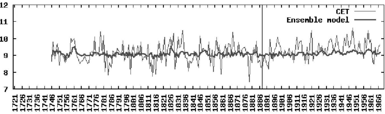
Finally, the filtered models were sorted according to their RMSE for the training set and an ensemble model was constructed (by simple averaging) with the three top models. The behavior of the ensemble model is shown in Fig.3 The ensemble model falls short at describing the observed CET values. This is not surprising, as solar activity is only one of the very many factors controlling Earth’s temperature. What is interesting is that a kind of background signal is obtained, which (for both the training and the validation set, this one never seen by the GP model), significantly correlates with the observations. Table.V. The correlations are not high and clearly not enough to derive far reaching inferences, but their statistical significance is at least suggestive.
TABLE V
RMSEANDCORRELATION COEFFICIENT FOR THE ENSEMBLE OF EXPERT MODELS CORRESPONDING TOEXP.1ANDEXP.3SUITES. CRITICAL𝑟𝑐AT THE𝛼= 0.5CONFIDENCE LEVEL. TRAINING SET:
𝑟𝑐= 0.1516 (D.F=165). CRITICAL𝑟𝑐FOR THE VALIDATION SET 𝑟𝑐= 0.2735 (D.F=53).(*)INDICATES SIGNIFICANCE AT THE𝛼= 0.5
CONFIDENCE LEVEL. RMSE
Experiment Training validation Number of suite predictor variables Exp.1 0.54929 0.54859 50 Exp.3 0.57345 0.56005 10 Correlation Coefficient Exp.1 0.385 (*) 0.345 (*) 50 Exp.3 0.197 (*) 0.321 (*) 10 B. Exp.2.a suite
The one-dimensional lag-importance function for all mod-els resulting from Exp.2.a is shown in Fig.4 (for the GSN and CET series). In order to select a subset of
Fig. 4. Lag Importance Spectrum corresponding to the single-window ex-periment covering the entire observation record. Top: GSN Lag Importance Spectrum (ℒ𝑤(𝑡, 𝜏
𝑝,𝑞) functions)). Horizontal axis is the time lag in years, Bottom half: CET spectrum importance values. Each of them contains25 lags.
more relevant lags, thresholds (𝑇𝑠) with values 0.5 and 0.6 were applied to the lag importance functions. The re-sulting subsets of relevant lags obtained with 𝑇𝑠 = 0.5
Fig. 3. Comparison of the observed CET record with an ensemble of experts model derived from the three best models obtained with GP under the experimental settings of Table.I and50 predictor variables. The vertical line divides the training and the validation sets. The correlations between the CET values and the Ensemble model for both the training and the validation sets were statistically significant at the 𝛼= 0.5 confidence level.
were 𝑔𝑠𝑛 : {1, 3, 6, 7, 15, 16, 17, 21, 23, 24, 25} and 𝑐𝑒𝑡 : {1, 2, 3, 4, 5, 6, 7, 8, 9, 11, 15, 17, 19, 20, 22, 23, 25} for a to-tal of28 predictor variables. The subsets obtained with 𝑇𝑠= 0.6 were 𝑔𝑠𝑛 : {3, 6, 7, 17, 24} and 𝑐𝑒𝑡 : {1, 15, 17, 23} for a total of 10 predictor variables. They represent a reduction factor of0.56 and 0.2 with respect to the original number of 50 predictor variables.
C. Exp.2.b suite
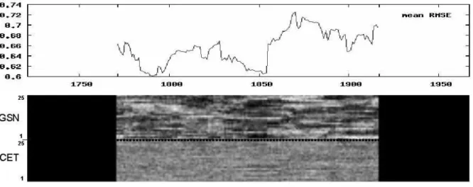
The two-dimensional lag importance function correspond-ing to the joint analysis of the CET and GSN series with MVTSMM and the parameter settings from Table.III is shown in Fig.5. Calendar time is on the x-axis and time lag value on the y-axis. The relative importance of the different time-lags is expressed by grey levels on the image (spectrum). For each spectrum the maximum time-lag is 25, increasing towards the top. MVTSMM has clearly produced a more textured structure for the GSN time-lags, leaving CET time-lags in a sort of non-differenciable noisy state. These changes are expressed in the mean RMSE function as well (Fig.5 top), indicating that the structure of the process does change with time. The presence of solar cycles 2 (1766-1775) and 4 (1784-1798) seem to still be present on the explanation of CET data until 1807. The end of the Dalton minimum (1790-1820) is also well marked. During 1843-1853, GSN time-lags 5, 12 and 24 seem to be the preferred, almost exclusivelly, while this is not the case for other periods. It seems that the GSN contribution to the CET data explanation, according MVTSMM analysis, follows a rather complex and changing pattern. Its interpretation and possible physical meaning, however, are outside the scope of the present paper.
D. Exp.3 suite
The subset of 10 lags derived from Exp.2.a when the threshold of 0.6 is applied to the 1-D lag importance func-tion, were used for a smaller series of GP model mining experiments. Model selection was made using the criteria described in VI-A and two models were found at the end of
the process. [296] 𝑇 (𝑡) =𝑘1+ 𝑇𝑡−17+ 𝑙𝑛(2 ∗ 𝑇𝑡−15) + 𝑙𝑛(𝑙𝑛(𝑙𝑛(𝑇𝑡−1))) −𝑙𝑛(𝑆𝑡−17+ 𝑆𝑡−16− 𝑇𝑡−15+ 𝑆𝑡−24∗ 𝑇𝑡−1 −𝑆𝑡−3∗ 𝑇𝑡−1+ 𝑒𝑇𝑡−17) (3) [385] 𝑇 (𝑡) =𝑘2+ 𝑙𝑛(𝑙𝑛(((𝑘4− 𝑆𝑡−16) + (𝑇𝑡−152 − 𝑆𝑡−24)))) +𝑇𝑡−1+ 𝑙𝑛(𝑇𝑡−1) + 𝑘3+ 𝑙𝑛(𝑇𝑡−15) − 𝑇𝑡−1 where 𝑘1 = 6.439965, 𝑘2= 6.954522, 𝑘3 = −3.966609, 𝑘4 = 237.173277. The numbered brackets on top of the models are only identifiers.
A model ensemble using those of Eq. 3 was constructed by simple average. Its behavior is shown in Fig.6 and Table.V. Although its correlation values are smaller than those of the ensemble obtained in Exp.1, they are also statistically significant. The RMSE values are only slightly larger, and again, it is interesting to observe that the model space explored here is considerably smaller (only 10 predicting variables were used). Note that from them only 7 variables (a further reduction) are included in the ensemble model (𝑔𝑠𝑛 : {3, 16, 17, 24}, and 𝑐𝑒𝑡 : {1, 15, 17}). Interestingly, they correspond to peak locations in the Lag Importance Spectra of Exp.2a (Fig. 5), not only to values above the0.6 threshold. The peaks are particularly well expressed in the GSN series, which is a proxy of solar activity. These results indicate that the chosen lags carry meaningful information.
VII. CONCLUSIONS
As the world’s largest temperature record, CET data has been subjected to intense research [1]. In spite of that, we believe that the techniques used in this paper could open a window to new possibilities for exploration. These are very preliminary results emerging from data mining of a very complex problem, which requires further investigation. Although suggestive, the connection of the results with real physical processes remains uncertain in spite of their very promising character. The models obtained are only function approximations which seem to be valid exploration tools for
Fig. 5. Top: mean RMSE for the models mined by MVTSMM for the corresponding period. Bottom: Lag importance spectra (ℒ𝑤(𝑡, 𝜏
𝑝,𝑞) functions)). Horizontal axis is time in years, vertical axis is the lag with respect to the current time position. The dotted line separates the two spectra. Upper half: GSN spectrum. Lower half: CET spectrum. Each of them contains25 lags.
Fig. 6. Comparison of the observed CET record with an ensemble of experts model derived from the two statistically significant models obtained with GP under the experimental settings of Table.III and only10 predictor variables, selected according to a threshold of 0.6 applied to the lag importance function obtained with MVTSMM. The vertical line divides the training and the validation sets. The correlations between the CET values and the Ensemble model for both the training and the validation sets were statistically significant at the 𝛼= 0.5 confidence level.
orienting further work. The use of these and other com-putational techniques on different suspected process-related data (with cross-checking), could provide new and interesting momenta in the global warming issue. The results obtained here are suggestive, but preliminary and further research is necessary. They should not be used to prove or disprove the possible physical mechanisms behind global warming.
VIII. ACKNOWLEDGEMENTS
The authors would like to thank Robert Orchard from the National Research Council Canada (Institute for Information Technology), David Kawrakow from McGill University and Ian Stakenvicius from Aerobiology Research for their sup-port, which made this research possible, and to the British Atmospheric Data Center which kindly provided the Central England Temperature series.
REFERENCES
[1] T. Benner. Central england temperatures: Long-term variability and teleconnections. Int. J. Climatol., 19:391–403, 1999.
[2] G. Box and G. Jenkins. Time Series Analysis, Forecasting and Control. Prentice Hall, 1976.
[3] E.J. Reichmann D.H. Hathaway, R.M. Wilson. Group sunspots numbers: Sunspot cycle characteristics. Solar Physics, 211:357–370, 2002.
[4] C. Ferreira. Gene expression programming: A new adaptive algorithm for problem solving. Journal of Complex Systems, 13(2):87–129, 2001. [5] C. Ferreira. Gene Expression Programming: Mathematical Modeling
by an Artificial Intelligence. Springer Verlag, 2006.
[6] W. Herschel. Observations tending to investigate the nature of the sun, in order to find the causes or symptoms of its variable emission of light and heat; with remarks on the use that may possibly be drawn from solar observations. Solar Physics, 91:265–318, 1801.
[7] D. V. Hoyt and K. H. Schatten. Group sunspot numbers: A new solar activity reconstruction. part 1.. Solar Physics, 181:491–512, 1998. [8] IPCC. Climate Change 2007: The Fourth Assessment Report.
WMO-UNEP, 2007.
[9] H. C. Koons and D. J. Gorney. A sunspot maximum prediction using a neural network. NASA STI/Recon Technical Report N, 91:13392–+, February 1990.
[10] J. Koza. Hierarchical genetic algorithms operating on populations of computer programs. In Proceedings of the 11th International Joint
Conference on Artificial Intelligence., pages 768–774, San Mateo, CA., 1989. Morgan Kaufmann.
[11] J. Koza. Genetic programming: On the programming of computers by
means of natural selection.MIT Press, 1992.
[12] J. Koza. Genetic programming ii: Automatic discovery of reusable
programs.MIT Press, 1994.
[13] J. Koza, D. Andre, and M. Keane. Genetic programming III:
Dar-winian invention and problem solving.Morgan Kaufmann, 1999. [14] P.S. Lucio. Changes in occurrences of meteorological extreme events
over continental portugal. In 5th Annual Meeting of the European
Meteorological Society / 7th European Conference on Applications of Meteorology., Utrecht, The Netherlands., 12-16 September 2005. [15] G. Manley. Central england temperatures: monthly means 1659 to
1973. Q.J.R. Meteorol. Soc., 100:389–405, 1974.
[16] Salvatore Marra and Francesco Carlo Morabito. A new technique for solar activity forecasting using recurrent elman networks. In C. Ardil, editor, Proceedings of the International Enformatika Conference,
IEC’05, pages 68–73, Prague, August 26-28 2005.
[17] Salvatore Marra and Francesco Carlo Morabito. Solar activity forecast-ing by incorporatforecast-ing prior knowledge from nonlinear dynamics into neural networks. In Proceedings of the International Joint Conference
on Neural Networks IJCNN 2006., pages 3722–3728, Vancouver, July 16-21 2006. IEEE.
[18] U. Naftaly, N. Intrator, and D. Horn. Optimal ensemble averaging of neural networks. Network, 8(3):283–296, 1997.
[19] D.E. Parker and E.B. Horton. Uncertainties in the central england temperature series since 1878 and some changes to the maximum and minimum series. Int. J. Clim, 25:1173–1188, 2005.
[20] V. Petridis and A. Kehagias. Neural Networks. Applications to Time
Series.Kluver, 1998.
[21] A. Pole, M. West, and J. Harrison. Applied Bayesian Forecasting and
Time Series Analysis. CRC, 1994.
[22] Muscheler R., Joosb F., Beer J., M¨uller S. A., Vonmoos M., and Snowball I. Solar activity during the last 1000 yr inferred from radionuclide records. Quaternary Science Reviews, 26(1-2):82–97, 2007.
[23] G. C. Reinsel. Elements of Multivariate Time Series Analysis. Springer Verlag, 1993.
[24] S.K.Solanki, I.G. Usoskin, B. Kromer, M. Sch¨ussler, and J. Beer. Unusual activity of the sun during recent decades compared to the previous 11,000 years. Nature, 431:1084–1087, 2004.
[25] H. Svensmark, T. Bondo, and J. Svensmark. Cosmic ray decreases af-fect atmospheric aerosols and clouds. Geophys. Res. Lett., 36(L15101), 2009.
[26] B. A. Tinsley. The global atmospheric electric circuit and its effects on cloud microphysics. Rep. Prog. Phys., 71(066801), 2008. [27] J.J. Vald´es. Time series models discovery with similarity-based
neuro-fuzzy networks and evolutionary algorithms. In Proceedings of the
IEEE World Congress on Computational Intelligence WCCI2002. 12 (5)., pages 2345–2350, 2002.
[28] J.J. Vald´es and A.J. Barton. Mining multivariate time series models with soft-computing techniques: A coarse-grained parallel computing approach. Lecture Notes in Computer Science. Springer-Verlag, 2668:259–268, 2003.
[29] J.J. Vald´es and G. Bonham-Carter. Time dependent neural network models for detecting changes of state in complex processes: Applica-tions in earth sciences and astronomy. Neural Networks, 19:196207, 2006.
[30] J.J. Vald´es and A. Pou. Greenland temperatures and solar activity: A computational intelligence approach. In Proceedings of the
Interna-tional Joint Conference on Neural Networks IJCNN 2007., Orlando, Florida., August 12-17 2007. IEEE.
[31] R. van Dorland. Scientific assessment of solar induced climate change. Technical report, The Royal Netherlands Meteorological Institute (KNMI)., The Royal Netherlands Institute for Sea Research (NIOZ)., 2006.
[32] J. Villarreal and P. Baffes. Sunspot prediction using neural networks.
NASA STI/Recon Technical Report N, 90:25560–+, March 1990. [33] J.X. Xie, C.T. Cheng, K.W. Chau, and Y.Z. Pei. A hybrid adaptive
time-delay neural network model for multi-step-ahead prediction of sunspot activity. International Journal of Environment and Pollution, 28(3/4):364–381, 2006.
[34] Eric Zhang and Paul Trimble. Predicting effects of climate fluctuations for water management by applying neural networks. World Resource