B → (ρ/ω) γ at BABAR
by
Karsten K¨oneke
Submitted to the Department of Physics
in partial fulfillment of the requirements for the degree of
Doctor of Philosophy in Physics
at the
MASSACHUSETTS INSTITUTE OF TECHNOLOGY
June 2007
c
° Massachusetts Institute of Technology 2007. All rights reserved.
Author . . . .
Department of Physics
May 25, 2007
Certified by . . . .
Gabriella Sciolla
Assistant Professor
Thesis Supervisor
Accepted by . . . .
Thomas J. Greytak
Associate Department Head for Education
B → (ρ/ω) γ at
B
A
B
AR
by
Karsten K¨oneke
Submitted to the Department of Physics on May 25, 2007, in partial fulfillment of the
requirements for the degree of Doctor of Philosophy in Physics
Abstract
This document describes the measurements of the branching fractions and isospin vio-lations of the radiative electroweak penguin decays B → (ρ/ω) γ at the asymmetric-energy e+e− PEP-II collider with the BABAR detector. Together with the previously
measured branching fractions of the decays B → K∗γ the ratio of CKM-matrix
elements |Vtd/Vts| are extracted and the length of the far side of the unitarity triangle
is determined.
Thesis Supervisor: Gabriella Sciolla Title: Assistant Professor
“[...] Daß ich erkenne, was die Welt Im Innersten zusammenh¨alt, [...]”[1]
Acknowledgments
To my family
First and foremost, I want to thank my family for their never ending support during all the years leading up to this thesis. I would have never come this far without them.
Furthermore, I want to thank my advisor for her support during the research leading up to the results presented in this document.
And off course I want to thank everyone who helped out academically or morally during the past years.
Contents
1 Introduction 16
1.1 Theoretical Motivation . . . 17
1.1.1 The Standard Model . . . 17
1.1.2 The CKM Matrix . . . 17
1.1.3 The B → (ρ/ω) γ Radiative Penguin Decay . . . . 19
1.2 Previous Measurements . . . 25
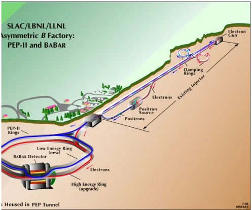
2 The BABAR Experiment 27 2.1 The Stanford Linear Accelerator Center . . . 27
2.2 The PEP-II Collider . . . 27
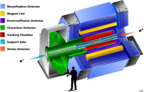
2.3 The BABARDetector . . . 29
2.3.1 The Silicon Vertex Tracker . . . 30
2.3.2 The Drift Chamber . . . 31
2.3.3 The Detector of Internally Reflected Cherenkov Light . . . 33
2.3.4 The Electromagnetic Calorimeter . . . 35
2.3.5 The Instrumented Flux Return . . . 36
2.4 Monte Carlo Simulation . . . 40
3 Analysis Overview 42 3.1 Introduction . . . 42
3.2 Event Signatures . . . 43
3.3 Major Backgrounds . . . 43
3.5 A Blind Analysis . . . 46 3.6 Data Samples . . . 46 3.6.1 Monte Carlo . . . 46 3.6.2 Data . . . 48 4 Event Reconstruction 49 4.1 Skim Requirements . . . 49
4.2 Event Level Requirements . . . 50
4.2.1 Tag Filter . . . 50
4.2.2 Number of Reconstructed Tracks . . . 52
4.2.3 R2 . . . 53
4.3 Photon Selection . . . 53
4.3.1 The GoodPhotonLoose List . . . 54
4.4 High Energy Photon Selection . . . 55
4.4.1 Energy of the High-Energy Photon . . . 55
4.4.2 Reconstruction Quality of the High-Energy Photon . . . 56
4.4.3 Geometric Acceptance . . . 56
4.4.4 Distance to Next Energy Deposition . . . 57
4.4.5 The 2nd Moment . . . . 57
4.4.6 Ratio of Energies Deposited in Crystals . . . 58
4.5 π0 Selection . . . . 58
4.6 π+ Selection . . . . 59
4.6.1 Particle Identification . . . 59
4.7 Vector Meson Selection . . . 61
4.7.1 Helicity Angle . . . 62
4.7.2 Dalitz Angle . . . 63
4.8 B Meson Selection . . . . 64
4.8.1 ∆E of the B Meson . . . . 64
4.8.2 mES of the B Meson . . . . 64
4.8.4 Analysis Regions . . . 68
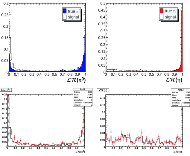
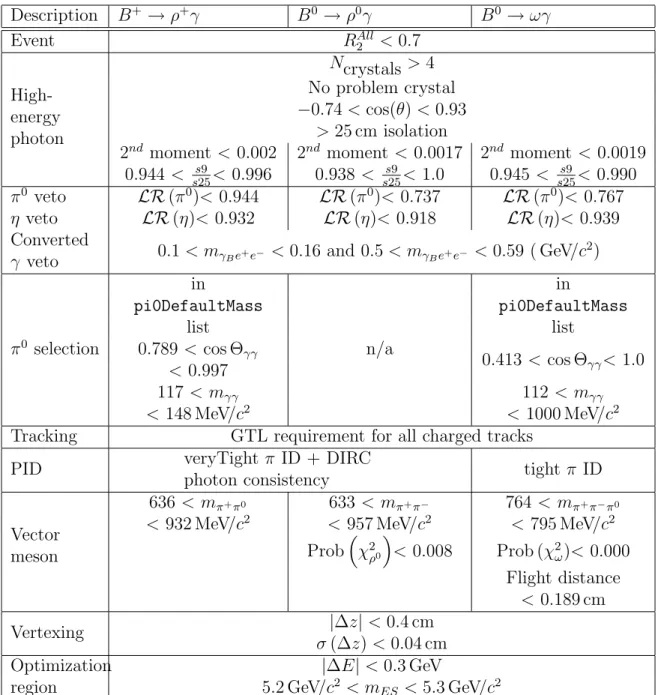
5 Background Suppression 69 5.1 π0 and η Veto for the High-Energy Photon . . . . 69
5.1.1 Likelihood Based Method . . . 70
5.1.2 Converted Photons . . . 72
5.1.3 Combined Veto Performance . . . 74
5.2 Background Suppression with a Neural Network . . . 77
5.2.1 Input Variables to the Neural Network . . . 77
5.2.2 Neural Network Algorithm and Training Implementation . . . 83
5.2.3 Neural Network Performance . . . 85
5.3 Cut Optimization . . . 88
5.3.1 Introduction . . . 88
5.3.2 The PRIM algorithm . . . 88
5.3.3 Method and Used Variables . . . 89
5.3.4 Resulting Cuts . . . 90
6 Expected Yields 93 7 Signal Extraction via a Maximum Likelihood Fit 100 7.1 Fit Overview . . . 100
7.2 Likelihood Function . . . 101
7.3 The B+ → ρ+γ Fit Model . . . 109
7.4 The B0 → ρ0γ Fit Model . . . 114
7.5 The B0 → ωγ Fit Model . . . 118
7.6 The Simultaneous Fit Models . . . 122
7.7 “Toy MC” Studies . . . 126
8 Systematic Errors 134 8.1 Tracking . . . 134
8.2 Charged Particle Identification . . . 135
8.4 π0 Selection . . . 138
8.5 π0/η Veto . . . 139
8.6 Neural Network . . . 143
8.7 Transformed Neural Network PDF Shape . . . 147
8.8 Signal PDF Parameter Corrections . . . 147
8.9 Signal PDF Shape . . . 156
8.10 B Background PDF . . . 156
8.11 B Counting . . . 157
8.12 ω → π+π−π0 Branching Fraction . . . 157
8.13 Simultaneous Fit Models . . . 157
8.14 Summary of Systematic Errors . . . 158
9 Results 159 9.1 Branching Fractions . . . 159 9.1.1 Fit Results . . . 160 9.1.2 Significance . . . 160 9.1.3 Upper Limit . . . 169 9.1.4 Summary . . . 169 9.2 Isospin . . . 171 9.3 CKM Parameters . . . 171 9.3.1 |Vtd/Vts| . . . 171 10 Conclusions 174 A Introduction to Neural Networks 178 A.1 Neural Network Training . . . 180
B Neural Network Input Variables 183 C Selection of Control Samples 196 C.1 B → Dπ for Neural Network Systematics . . . 196
E Used Functions 201
E.1 The Gaussian Function . . . 201
E.2 The Novosibirsk Function . . . 201
E.3 The Crystal Ball Function . . . 202
E.4 The Cruijff Function . . . 202
List of Figures
1-1 The CKM unitarity triangle. . . 19
1-2 Feynman diagram for the b → dγ transition. . . . 20
1-3 Effective Feynman diagram for the b → dγ transition. . . . 21
1-4 Second order contributions to the B → (ρ/ω) γ decay. . . . 22
1-5 Feynman diagram for B ¯B oscillations. . . . 23
2-1 A schematic overview of the experimental site at SLAC. . . 28
2-2 The PEP-II storage ring. . . 29
2-3 The BABARdetector. . . 30
2-4 The BABARSilicon Vertex Tracker (side view). . . 31
2-5 The BABARdrift chamber (side view). . . 32
2-6 A charged particle moving perpendicular to a magnetic field. . . 33
2-7 The BABARDetector of Internally Reflected Cherenkov Light (side view). 34 2-8 The BABARElectromagnetic Calorimeter (side view). . . 35
2-9 The BABARInstrumented Flux Return. . . 37
2-10 The BABARResistive Plate Counters. . . 37
2-11 The BABARLimited Streamer Tubes. . . 39
3-1 Event signatures. . . 45
4-1 Illustration of the second moment variable. . . 58
4-2 Graphical representation of the helicity angle. . . 62
4-3 ∆E and mES for B0 → ρ0γ signal MC. . . . 65
4-4 Comparison of the resolution of m0
5-1 Background Composition. . . 70
5-2 Distributions of MγBγ2 (left) and Eγ2 (right) for truth matched signal events, and high-energy photons originating from π0 and η decays. . . 71
5-3 π0 and η likelihood ratios for MC and off-resonance data for the ρ0mode. 73 5-4 mγBe+e− distributions for MC. . . 74
5-5 π0/η veto efficiencies for different veto methods. . . . 75
5-6 Resulting neural network performance. . . 86
7-1 Correlations between fit dimensions for B+→ ρ+γ for signal MC. . . 103
7-2 Correlations between fit dimensions for B+→ ρ+γ for continuum MC. 104 7-3 Correlations between fit dimensions for B0 → ρ0γ for signal MC. . . . 105
7-4 Correlations between fit dimensions for B0 → ρ0γ for continuum MC. 106 7-5 Correlations between fit dimensions for B0 → ωγ for signal MC. . . . 107
7-6 Correlations between fit dimensions for B0 → ωγ for continuum MC. 108 7-7 The PDFs used in the B+ → ρ+γ fit model. . . 112
7-8 Comparison of transformed neural network shapes for the B+ → ρ+γ fit model. . . 113
7-9 The PDFs used in the B0 → ρ0γ fit model. . . 116
7-10 Comparison of transformed neural network shapes for the B0 → ρ0γ fit model. . . 117
7-11 The PDFs used in the B0 → ωγ fit model. . . 120
7-12 Comparison of transformed neural network shapes for the B0 → ωγ fit model. . . 121
7-13 Signal embedded toy MC studies for the B+ → ρ+γ fit model. . . 129
7-14 Signal embedded toy MC studies for the B0 → ρ0γ fir model. . . 130
7-15 Signal embedded toy MC studies for the B0 → ωγ fit model. . . 131
7-16 Signal embedded toy MC studies for the three decay mode simultane-ous fit model. . . 132
8-1 Charged particle identification performance. . . 136
8-3 mES distributions for B− → D0π−, D0 → K−π+ and B0 → D−π+,
D−→ K+π−π−. . . 140
8-4 Comparison of π0 and η vetoes between B− → D0π−, D0 → K−π+ data and MC. . . 141
8-5 Comparison of π0 and η vetoes between B0 → D−π+, D− → K+π−π− data and MC. . . 142
8-6 Neural network output comparison between data and MC. . . 144
8-7 Comparison of B → Dπ neural network distributions for MC and background subtracted on–resonance data. . . 145
8-8 Signal efficiencies and efficiency ratios. . . 146
8-9 Step function PDFs used for the three decay modes. . . 148
8-10 Differences in the signal yield between using the nominal fits and fits using step function PDFs for the transformed neural network output. 149 8-11 PDF shapes used in B → K∗0γ (K∗0 → Kπ) fit . . . 150
8-12 PDF shapes used in B → K∗+γ (K∗+ → K+π0) fit . . . 151
8-13 Projection plots for weighted MC B → K∗0γ (K∗0→ K+π−) fit . . . 152
8-14 Projection plots for on-peak data B → K∗0γ (K∗0 → K+π−) fit . . . 152
8-15 Projection plots for weighted MC B → K∗+γ (K∗+ → K+π0) fit . . . 153
8-16 Projection plots for on-peak data B → K∗+γ (K∗+ → K+π0z) fit . . 153
9-1 Projections for the ρ+ mode. . . 162
9-2 Projections for the ρ+ mode. . . 163
9-3 Projections for the ρ0 mode. . . 164
9-4 Projections for the ρ0 mode. . . 165
9-5 Projections for the ω mode. . . 166
9-6 Projections for the ω mode. . . 167
9-7 Likelihood curves (-2log L/Lmax) for the fit results. . . 168
9-8 Summary of branching fraction measurements from BABARand Belle. 170 9-9 The far side of the unitarity triangle Rt. . . 173
A-1 A one dimensional cut. . . 179
A-2 A two dimensional cut compared to a neural network. . . 180
A-3 Neural network visualization. . . 181
B-1 Separation power of the input variables to the neural networks. . . 184
B-2 Separation power of the input variables to the neural networks. . . 185
B-3 Separation power of the input variables to the neural networks. . . 186
B-4 Separation power of the input variables to the neural networks. . . 187
B-5 Separation power of the input variables to the neural networks. . . 188
B-6 Separation power of the input variables to the neural networks. . . 189
B-7 Data-MC agreement of the input variables to the neural networks. . . 190
B-8 Data-MC agreement of the input variables to the neural networks. . . 191
B-9 Data-MC agreement of the input variables to the neural networks. . . 192
B-10 Data-MC agreement of the input variables to the neural networks. . . 193
B-11 Data-MC agreement of the input variables to the neural networks. . . 194
B-12 Data-MC agreement of the input variables to the neural networks. . . 195 C-1 The likelihood fit on the B → Dπ on–resonance data control samples. 198
List of Tables
1.1 Next to leading order predictions for B → (ρ/ω) γ decay modes. . . . 24
1.2 Current experimental results for B(B → ργ) and B(B → ωγ). . . . . 25
1.3 Assumed branching fractions for this analysis. . . 26
3.1 Signal Monte Carlo modes used in this analysis. . . 47
3.2 Generic Monte Carlo modes used in this analysis. . . 47
3.3 Data used in this analysis. . . 48
5.1 Veto efficiencies for off-resonance data and continuum MC. . . 76
5.2 NN input variables. . . 84
5.3 Analysis cuts applied prior to the training of the final neural networks. 87 5.4 Neural network architecture for the three decay modes. . . 87
5.5 Fixed cuts applied before optimization is carried out for the remaining criteria. . . 89
5.6 Summary of optimized selection criteria for B+ → ρ+γ. . . . 91
5.7 Summary of optimized selection criteria for B0 → ρ0γ. . . . 91
5.8 Summary of optimized selection criteria for B0 → ωγ. . . . 91
5.9 Summary of Bump Hunter performance. . . 92
6.1 B+ → ρ+γ signal MC efficiency table. . . . 94
6.2 B0 → ρ0γ signal MC efficiency table. . . . 95
6.3 B0 → ωγ signal MC efficiency table. . . . 96
6.4 Expected yield for the B+→ ρ+γ decay mode. . . . 97
6.6 Expected yield for the B0 → ωγ decay mode. . . . 99
7.1 Fit region cuts and signal efficiencies for all three decay modes. . . 101
7.2 Expected number of events in the fit region for all three decay modes. 102 7.3 PDFs used in the B+ → ρ+γ fit model. . . 109
7.4 B background normalizations used for the B+ → ρ+γ fit model. . . . 110
7.5 PDFs used in the B+ → ρ+γ fit model. . . 114
7.6 B background normalizations used for the B0 → ρ0γ fit model. . . 115
7.7 PDFs used in the B0 → ωγ fit model. . . 118
7.8 Fit results of embedding different number of signal events. . . 128
7.9 Fit summary. . . 133
8.1 The µµγ data/MC efficiency ratios for the photon quality selection. . 139
8.2 Summary of data and MC fits to B → K∗0γ (K∗0→ K+π−) sample. 155 8.3 Summary of data and MC fits to B → K∗+γ (K∗+ → K+π0) sample. 155 8.4 Fractional systematic errors (in %) of the measured branching frac-tions. . . 158
9.1 Results of the five fits. . . 161
9.2 Summary of the results. . . 170
C.1 Dataset used in the neural net validation. . . 196
C.2 Signal efficiencies and expected yields for the B → Dπ control samples using the Run1-5 data set. . . 197
Chapter 1
Introduction
Currently, two high precision experiments designed to study the B meson sector are in operation: BABAR and Belle. Both experiments are operating at asymmetric
energy electron-positron colliders running at a center of momentum (CM) energy of 10.58 GeV. This energy corresponds to the mass of the Υ(4S) resonance, a meson which is a bound state of a b quark and an anti-b quark in the 4S configuration. Both
BABAR and Belle are high luminosity experiments with a current peak luminosity of
1.21 · 1034cm−2s−1 and 1.65 · 1034cm−2s−1 respectively.
Also, there is data available from the CLEO collaboration, the previous-generation experiment studying B mesons at an e+e−collider. This experiment was a symmetric
machine also running at the Υ(4S) resonance. It was acquiring data at a much lower rate, the peak luminosity was about 8.5 · 1032cm−2s−1.
Furthermore, the two detectors at the Tevatron, CDF and D∅, are also studying the physics in the b quark sector. These two experiments are not as clean as the other three mentioned above since the Tevatron is a hadron collider and thus the initial state is not known like it is in the e+e− machines. Also, there are a lot more
final state particles in a hadron collider than in a e+e− collider. Thus it is much
harder to isolate a photon from the rest of the event which will be needed for this analysis. But the Tevatron can measure another quantity, the oscillation frequency of Bs mixing, where the Bs meson is a bound state of a b anti-quark and an s quark.
of the decay B → (ρ/ω) γ are tied to the same quantities according to our current understanding of elementary particle physics, the Standard Model. Thus, these two measurements should come to the same conclusions, if the Standard Model is correct.
1.1
Theoretical Motivation
1.1.1
The Standard Model
Today’s understanding of the physics of elementary particles is described in terms of the Standard Model of Elementary Particle Physics (SM). This model is dealing with two types of spin-1
2 particles (quarks and leptons) and three types of forces (strong,
electromagnetic and weak force). The forces are mediated by three different types of force carriers: 8 gluons, the photon, and the W± and Z0 vector (=spin-1) bosons,
respectively. The SM is a gauge theory. The invariance of the SM lagrangian under local transformation belonging to the U(1)Y ⊗ SU(2)L group yields the electroweak
part of the SM, while the local transformation belonging to the SU (3)C group leads to
the part of the SM dealing with strong interactions, as described by Quantum Chromo Dynamics (QCD). To be more precise, the required invariance of the lagrangian under these local gauge transformations leads to the three types of force carriers, the vector bosons. Therefore, these force carriers are also known under the name “gauge bosons”. Up to now, the theoretical predictions of the SM agree to a high precision with experimental measurements. Deviations are expected at some (unknown) level since this model is intrinsically incomplete. It becomes inconsistent at high energies of about 1 TeVand higher.
1.1.2
The CKM Matrix
In the SM, the quark mass (or flavor) matrices are in general not diagonal. In order to transform the quark flavor states into the weak eigenstates needed in the lagrangian, one performs a rotation in the quark flavor space. This rotation of the flavor eigen-states leads to the diagonal weak eigeneigen-states which are used in the lagrangian. This
leads to a non-vanishing rotation matrix in the weak charged current term of the lagrangian, the Cabibbo-Kobayashi-Maskawa (CKM) matrix. This unitary matrix is usually interpreted as a redefinition of the down-type eigenstates of the weak interac-tion (primed) as a linear combinainterac-tion of the down-type flavor eigenstates (unprimed).
d0 s0 b0 = VCKM · d s b = Vud Vus Vub Vcd Vcs Vcb Vtd Vts Vtb · d s b (1.1)
This CKM matrix is a unitary complex matrix and it has for the case of three quark generations 18 parameters. But since the matrix is unitary, only nine of these 18 parameters are independent. Furthermore, one can always redefine the individual phases of the six quark fields and thus remove five more independent parameters. This leaves us with four independent parameters, three real parameters (angles) and one irreducible phase factor. This phase factor is the source of CP violation in the SM.
With this remaining four independent parameters, one can expand the CKM ma-trix in the so-called Wolfenstein parameterization of the CKM mama-trix [2][3]:
Vud Vus Vub Vcd Vcs Vcb Vtd Vts Vtb = 1 − 1 2λ2 λ Aλ3(ρ − iη) −λ 1 −1 2λ2 Aλ2
Aλ3(1 − ρ − iη) −Aλ2 1
+ O(λ 4). (1.2)
The unitarity conditions of the CKM matrix are
3 X i=1 VjiVki∗ = 0 = 3 X i=1 VijVik∗ for j 6= k. (1.3)
These can be visualized with six triangles. But for only two of those the length of all three sides are of the same order of λ (λ ≈ |Vus| ≈ |Vcd| ≈ 0.22). One of these two
triangles is usually referred to as “The Unitary Triangle”. This triangle originates from the CKM unitarity condition for the first and third column of the CKM matrix,
i.e., the ones relevant in the B meson system
VudVub∗ + VcdVcb∗+ VtdVtb∗ = 0. (1.4)
The triangle is furthermore normalized by dividing the above condition by VcdVcb∗.
This final standard unitarity triangle is shown in Figure 1-1 in the (¯ρ, ¯η) plane where
¯
ρ and ¯η are related to the usual Wolfenstein parameters as
¯ ρ = ρ −1 2ρλ2+ O (λ4) ¯ η = η −1 2ηλ2+ O (λ4) . (1.5)
R =
t(
ρ,η)
γ
α
β
ρ
η
R =
u(0,0) (1,0)
V
udV
ub*V
cdV
cb*V
tdV
tb*V
cdV
cb*Figure 1-1: The CKM unitarity triangle. Modified from [4].
1.1.3
The B → (ρ/ω) γ Radiative Penguin Decay
A penguin decay is a flavor changing neutral current (FCNC) process. FCNC processes in the SM only take place at higher order, i.e., with at least one loop in the Feyn-man diagram. The name “penguin decay” was first used as a result of a bet in [5]. In the case of B → (ρ/ω) γ, a W boson and an up-type quark are in the loop (see
Figure 1-2).
b u,c,t d
W
γ
Figure 1-2: Feynman diagram for the b → dγ transition. This is the leading order “penguin” diagram for this transition.
There are several motivations to study B → (ρ/ω) γ (and also B → K∗γ) decays.
These decays proceed at leading order via an electroweak penguin loop shown in Figure 1-2. Since the top-quark penguin diagrams are the largest contributions to these processes, the measurement of observables in these decays are probes of the top-quark couplings.
Theory Framework
In order to compute observables of the decay B → (ρ/ω) γ, an effective theory is used. In this particular case, the heavy quark effective theory is used. This effective theory integrates out the heavy fields from the full theory. The effective interaction Hamiltonian is [6] Hef f = −4G√F 2 V ∗ tdVtb 10 X i=1 Ci(µ)Oi(µ) , (1.6)
where GF is the Fermi constant, Vtj are CKM matrix elements, Ci(µ) are Wilson
coefficient (dependent on the renormalization scale µ) and Oi(µ) are the operators.
Unitarity of the CKM matrix has been assumed and everything beyond leading order in αem, mb/mW, md/mb and Vub/Vcb has been neglected. The short distance QCD
effects due to hard gluon exchanges between the quark lines of the leading order one loop Feynman diagram is contained in the Wilson coefficients which can be calculated perturbativly. The Hamiltonian relates the final ρ/ω meson state to the initial B meson state.
b d γ
Figure 1-3: Effective Feynman diagram for the b → dγ transition. After integrating out the heavy degrees of freedom, this effective diagram remains.
W boson) from the dominant Feynman diagram shown in Figure 1-2, the effective
Feynman diagram shown in Figure 1-3 remains. This diagram is described in the Hamiltonian (see Equation 1.6) by
O7(µ) = e mb(µ) 8π2 ¡¯ dασµν(1 + γ5) bα ¢ Fµν, (1.7)
where bα is the initial b quark state, ¯dα is the final d quark state, Fµν is the photon
field strength tensor, e is the electromagnetic coupling constant, mb(µ) is the
scale-dependent b quark mass and σµν is the only possible antisymmetric tensor needed to
contract Fµν with. In fact, this is the simplest possible operator that describes the
transition of a b quark into a d quark and a photon. Ratio of Branching Fractions and |Vtd/Vts|
The ratio of the CKM matrix elements Vtd/Vts can be calculated from the ratio of
branching fractions of the two exclusive radiative penguin decays B → (ρ/ω) γ and
B → K∗γ [7]: B(B → ργ) B(B → K∗γ) = Sρ ¯ ¯ ¯ ¯VVtd ts ¯ ¯ ¯ ¯ 2 ¡1 − m2 ρ/M2 ¢3 (1 − m2 K∗/M2)3 ζ2[1 + ∆R(ρ/K∗)] (1.8) where ζ = ξ⊥ρ(0)/ξK∗
⊥ (0) is the ratio of form factors computed in Heavy Quark
Ef-fective Theory (HQET), Sρ = 1(1/2) are isospin weights for the charged (neutral)
ρ meson and ∆R(ρ/K∗) is a dynamical function calculated for example in [7] which
accounts for different dynamics in the three decays like vertex, hard-spectator, weak annihilation or weak exchange contributions. The weak annihilation contribution to
the B+→ ρ+γ decay and the W exchange contribution to the neutral B meson decay
are shown in Figure 1-4.
W
¯b
u
u
¯
d
γ
¯b d ¯ u u W γFigure 1-4: Second order contributions to the B → (ρ/ω) γ decay. The Feynman diagram on the left shows the weak annihilation contribution to the B+→ ρ+γ decay
mode and the Feynman diagram on the left shows the W exchange contribution to the neutral B meson decay.
The latest theory calculation [8] (based on Light-Cone Sum Rules) of the ratio of form factors gives
ξρ= ζρ−1 = T1B→K∗(0) T1B→ρ(0) = 1.17 ± 0.09 (1.9) and ξω = ζω−1 = T1B→K∗(0) T1B→ω(0) = 1.30 ± 0.10. (1.10)
Reference [9] argues that ∆R(ρ/K∗) is actually depending on both QCD and
CKM parameters. In particular, for the determination of this quantity, a set of input parameters Rb and γ is needed where
Rb = µ 1 − λ2 2 ¶ 1 λ ¯ ¯ ¯ ¯VVubcb ¯ ¯ ¯ ¯ (1.11)
is the short side of the unitarity triangle and γ is the angle between that side and the base of the unitarity triangle. This puts ∆R(ρ/K∗) in the neighborhood of 0.1 ± 0.1,
but for the actual determination of the branching fraction ratio, the full description with appropriate errors has been used.
This same ratio of CKM matrix elements is determined from the ratio of ∆md/∆ms
where ∆m(d/s) are matter-antimatter oscillation frequencies of the neutral B(d/s)
Feyn-¯
s
b
¯b
¯
u, ¯c, ¯t
u, c, t
s
Figure 1-5: Feynman diagram for B ¯B oscillations.
man diagram shown in Figure 1-5. The oscillation frequency of the Bd system has
been precisely measured by the B-Factories [10, 11, 12, 13, 14, 15, 16, 17] while the oscillation frequency of the Bssystem has been recently measured by the CDF
collab-oration [18]. Even though the underlying dynamics of B ¯B oscillations and radiative
penguin decays are very different, in the framework of the SM, both ways of measur-ing |Vtd/Vts| yield the same result. It would be a clear indication of physics beyond
the SM if a difference is found between these two independent results. Branching Fractions
One can easily imagine a new (e.g. supersymmetric) particle in the penguin loop. This non-SM physics contribution could change the branching fraction of this decay measurably, but it does not necessarily change the ratio of branching fractions between
B → (ρ/ω) γ and B → K∗γ decays if the new particle couples the with the same
strength to the s and d quark. If this would be the case, the new physics contributions would be better visible in the B → K∗γ case due to the larger branching fraction.
If the couplings are different, e.g., only slightly effecting the B → K∗γ branching
fraction, but significantly effecting the B → (ρ/ω) γ branching fraction, then this would be visible in the determination of the ratio of branching fractions discussed above. Thus the actual measured value of the branching fractions is, taken on its own, less interesting due to the large theory uncertainties. These large uncertainties of theoretical calculations (see Table 1.1) are due to difficulties in calculating the hadronization of the final state mesons. Also QCD corrections to the penguin loop
itself are hard to compute.
Calculation B(B+→ ρ+γ) B(B0→ ρ0γ) B(B0 → ωγ)
Ali & Parkhomenko [19] 1.37 ± 0.26(th.) ±
0.09(exp.)
0.65 ± 0.12(th.) ± 0.03(exp.)
0.53 ± 0.12(th.) ± 0.02(exp.)
Bosch & Buchalla [20] 1.58+0.53−0.46 0.76+0.26−0.23
Ball, Jones & Zwicky [9] 1.16 ± 0.26 0.55 ± 0.13 0.44 ± 0.10
Table 1.1: Next to leading order predictions for the B → (ρ/ω) γ decay modes. All branching fractions are in units of 10−6.
Besides the already mentioned transitions of the type b → sγ, there are other decays related to B → (ρ/ω) γ. Two of these decays are B0 → φγ and B0 → J/ψ γ.
The difference is that these decays proceed at leading order via the annihilation type Feynman diagrams. Thus their branching fractions are expected to be unobservable at the current B factories. Based on the SM, they are expected to be B (B0 → φγ) =
¡
2.7+0.3+1.2−0.6−0.6¢× 10−11 and B (B0 → J/ψ γ) = ¡4.5+0.6+0.7
−0.5−0.6
¢
× 10−7 [21]. Even though
the later branching fraction is sizable, the branching fraction of B (J/ψ → l+l−) =
(5.94 ± 0.06) % [22] (where l+ = e+, µ+) is too small to allow for a detection of this
decay at the current B factories. The CKM Angle α
The CKM angle α is the angle at the apex of the unitarity triangle. It is defined as
α ≡ arg · −VtdVtb∗ VudVub∗ ¸ , (1.12)
where Vij are CKM matrix elements. Since the weak annihilation diagram (see
Fig-ure 1-4) contributing to the B+ → ρ+γ decay is proportional to V
udVub∗ and the top
quark dominated penguin diagram (see Figure 1-2) is proportional to VtdVtb∗, the ratio
of these two diagrams is proportional to
VubVud∗ VtbVtd∗ = − ¯ ¯ ¯ ¯VubV ∗ ud VtbVtd∗ ¯ ¯ ¯ ¯ eiα. (1.13)
Thus, the ratio of branching fraction of B+ → ρ+γ to B0 → ρ0γ is dependent on
α. More precisely, the quantity measuring isospin violation between the two decays B+ → ρ+γ and B0 → ρ0γ defined as
∆ ≡ Γ(B+ → ρ+γ)
2Γ(B0 → ρ0γ) − 1 (1.14)
is sensitive to cos α [19].
1.2
Previous Measurements
Prior to this analysis, only the Belle collaboration found a positive result in one channel, namely an approximately five sigma result in the neutral B0 → ρ0γ decay
mode. No other experiment was able to observe this decay mode nor has any of the other two decay modes (B+ → ρ+γ and B0 → ωγ) been observed. This situation is
summarized in Table 1.2.
Experiment B(B+ → ρ+γ) B(B0 → ρ0γ) B(B0 → ωγ) Combined result
CLEO[23] < 13 < 17 < 9.2
BABAR[24] < 1.76 < 0.36 < 0.97 < 1.16
BELLE[25] 0.55+0.42
−0.36 +0.09−0.08 1.25+0.37−0.33 +0.07−0.06 0.56+0.34−0.27 +0.05−0.10 1.32+0.34−0.31 +0.10−0.09
Table 1.2: Current experimental results for B(B → ργ) and B(B → ωγ). Limits are shown at 90% confidence level. The Belle paper [25] does not provide upper limits for the ρ+ and ω modes. Where appropriate, the first error is statistical, the second
systematic. All numbers are in units of 10−6.
For this analysis the charged decay mode B+→ ρ+γ is assumed to have a
branch-ing fraction of 1.0 · 10−6 and the branching fractions of both neutral decay modes
B0 → ρ0γ and B0 → ωγ are assumed to be 0.5 · 10−6 as summarized in Tabel 1.3.
This values are used for the purpose of optimizing the analysis, i.e., for selecting cuts, choosing the fit strategy, etc.
Mode Assumed branching fractions
B+ → ρ+γ 1.0 · 10−6
B0 → ρ0γ 0.5 · 10−6
B0 → ωγ 0.5 · 10−6
Chapter 2
The B
AB
ARExperiment
The BABARexperiment is based on an asymmetric energy e+e−collider at the Stanford
Linear Accelerator Center (SLAC) operating at a center of momentum (CM) energy of 10.58 GeV, coinciding with the Υ(4S) resonance. BABAR started taking data in
1999 and will continue running until fall of 2008.
2.1
The Stanford Linear Accelerator Center
The Stanford Linear Accelerator Center (SLAC) was established in 1962 and is located in Menlo Park, California. In 1966, the main linear accelerator (Linac)went into operation. This is a three kilometer long electron and positron accelerator now used to inject the electron and positron beams into the PEP-II storage rings. The linac is still the world’s largest and most powerful linear accelerator and it can provide beam energies of up to about 50 GeV. A schematic overview of the experimental site at SLAC can be seen in Figure 2-1.
2.2
The PEP-II Collider
The PEP-II collider is a two storage ring machine. One ring is an upgrade of the previously existing PEP collider which now stores a 9.0 GeV electron beam. The second storage ring is a new ring storing a 3.1 GeV positron beam. The PEP-II
Figure 2-1: A schematic overview of the experimental site at SLAC. Courtesy of Stanford Linear Accelerator Center.
collider was completed in July 1998.
The different energies of the electron and positron beams result into a CM frame which is moving in the laboratory frame with a Lorentz boost βγ = 0.56. This boost is crucial to study the B-meson system. Since the Υ(4S) is only about 22 MeV heavier than the two resulting B-mesons, the B-mesons are produced almost at rest in the Υ(4S) rest frame. But with the above mentioned Lorentz boost of the CM frame (which is the Υ(4S) rest frame), it is possible to measure the difference in the decay length of the two B-mesons which is due to a difference in their decay times. The Lorentz boost results in a spacial separation along the z-axis of the two B meson decay vertices of ∆z ≈ 250 µm.
The design peak luminosity of the PEP-II collider is 3 × 1033cm−2s−1. As of
today, the PEP-II record is 12.069 × 1033cm−2s−1, achieved August 16th 2006, which
already exceeds the design goal by a factor of four. The production cross section of
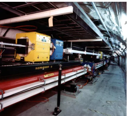
Figure 2-2: The PEP-II storage ring. The upper ring is the low energy positron ring and the lower ring is the high energy electron ring. Courtesy of Stanford Linear Accelerator Center.
million Υ(4S) produced by PEP-II each year.
The two beams in the PEP-II machine collide head on, i.e., there is no crossing angle at the interaction point (IP). And the time between two bunch crossings is 4.2 ns. A picture of the PEP-II storage ring is shown in Figure 2-2.
2.3
The B
AB
ARDetector
The BABARdetector is a modern high energy particle detector designed specifically for
an asymmetric electron positron collider running at the Υ(4S) resonance. Because of the boost along the e− direction, the detector is asymmetric with respect to the
collision point. The forward-backward asymmetry of the detector is designed in such a way that it covers approximately the same solid angle in the forward and backward direction in the CM frame.
a particle produced at the interaction point in the center of the detector to the outermost part of the detector. A schematic overview of the BABARdetector with its
subsystems can be seen in Figure 2-3. The information in these sections is coming mostly from “The BABAR Physics Book” [26] and “The BABAR Detector” [27].
Figure 2-3: The BABARdetector. Courtesy of Stanford Linear Accelerator Center.
2.3.1
The Silicon Vertex Tracker
The silicon vertex tracker (SVT) is the innermost part of the BABAR detector. It
consists of five layers of planar silicon detectors ordered in a cylindrical geometry around the beam axis at the interaction point. The innermost layer is in radial direction only 3.3 cm away from the interaction point and the outermost layer is 14.6 cm away. The SVT provides a spatial resolution in the z-direction of less than 70 µm [27] which is absolutely crucial in order to be able to resolve the separated vertices for the two mesons and thus being able to study CP-violation in the B-meson system. The resolution in the x-y plane is better than 100 µm.
580 mm 350 mrad 520 mrad e e- + Beam Pipe Space Frame Fwd. support cone Bkwd. support cone Front end electronics
Figure 2-4: The BABARSilicon Vertex Tracker [27] (side view).
2.3.2
The Drift Chamber
The BABAR drift chamber (DCH) is a 280 cm long cylinder with an inner radius of
23.6 cm and an outer radius of 80.9 cm (see Figure 2-5). The drift chamber is, like other parts of the detector, asymmetric in the forward-backward design in order to account for the asymmetric beam energies. The wires in the tracking volume are arranged in 10 super-layers of 4 layers of wires each, summing up to a total of 40 layers of wires. The super-layers have a slightly different orientation with respect to each other in order to be able to achieve a three-dimensional track reconstruction. The first super-layer is oriented exactly along the beam axis, the second and third one are tilted with an opposite angle with respect to the beam axis. The fourth layer is again oriented along the beam axis and this pattern is continued until the last super-layer is again oriented along the beam axis. The volume around the wires is filled with a Helium-based drift gas. A schematic overview of the DCH is shown in Figure 2-5.
With this configuration, the drift chamber performance for spatial resolution is better than 140 µm. Charged particles produced at the interaction point need at least a transverse momentum of about 100 MeV in order to reach the DCH. The tracking device (SVT and DCH) is located inside of an axial 1.5 T magnetic field.
From the curvature of a reconstructed track in the tracking systems of the BABAR
IP 1618 469 236 324 1015 1749 68 551 973 17.19 202 35
Figure 2-5: The BABAR drift chamber (side view). All measurements are in units of
millimeter.
The resolution in the transverse momentum is found to be [27]
σpt
pt
= (0.13 ± 0.01) % · pt+ (0.45 ± 0.03) %. (2.1)
The Lorentz force acting on a particle with charge q and velocity ~v propagating in a magnetic field ~B is (without the presence of an electric field)
~ FLorentz = q ³ ~v × ~B ´ . (2.2)
The centripetal force on a particle with mass m moving with momentum ~p on a curvature with radius r can be deduced with Newton’s second law
~ F = d~p
dt (2.3)
and the infinitesimal change in momentum direction d~p by an angle d~θ
d~p = ~p × d~θ , (2.4)
dθ p p+dp p p+dp dθ dp
Figure 2-6: A charged particle moving perpendicular to a magnetic field.
~ Fcentripetal = d~p dt = ~p × d~θ dt = −~p |~v| r . (2.5)
Since both forces have equal magnitude and opposite directions, one can combine these two equations in order to get a relation between the charge q and the momentum
~p of the particle, the magnetic field, the angle between magnetic field and particle
momentum αB−~~ p and the radius of the track curvature
|~p| = rq ¯ ¯ ¯ ~B ¯ ¯ ¯ sin αB−~~ p . (2.6)
2.3.3
The Detector of Internally Reflected Cherenkov Light
The detector of internally reflected Cherenkov light (DIRC) is designed to separate charged kaons from charged pions. If a charged particle travels in a medium faster than the speed of light in that medium, it emits Cherenkov light. The relation between the momentum of the charged particle and the angle between the particle’s flight direction and the Cherenkov light cone emission angle is
cos θCherenkov =
1
βn , (2.7)
where n = 1.473 is the refraction index of the medium and β is the velocity of the charged particle normalized to the vacuum speed of light.
Mirror 4.9 m 4 x 1.225m Bars glued end-to-end Purified ater edge Track Tra ectory 17.25 mm Thickness (35.00 mm idth) Bar Box PMT + Base 10,752 PMT s Light Catcher PMT Surface indow Standoff Box Bar 1.17 m 8-2000 8524A6
Figure 2-7: The BABARDetector of Internally Reflected Cherenkov Light (side view)
[27].
The DIRC is an array of 4.9 m long, 3.5 cm wide and 1.7 cm high bars made of synthetic fused silica, a translucent material in which Cherenkov light can be produced. There are a total of 144 bars arranged in 12 groups of 12 bars each. The Cherenkov light travels inside these bars towards a toroidal water tank at the backward end of the detector. The emission angle is preserved in these internat reflections due to the high accuracy of the parallel quartz-bar surfaces. Finally, an array of photomultiplier tubes detects the Cherenkov light at the backward end of this water tank. From the position and time of the detection in the photomultiplier tubes, an image of the initially produced Cherenkov light cone is inferred. This process is illustrated in Figure 2-7.
The separation between charged pions and kaons relies on their different masses. Particles with the same momentum but with different masses have different velocities and thus produce Cherenkov light at different angles. The separation only works if the charged particles are faster than the speed of light in the bars. A charged pion starts producing Cherenkov light if its momentum is larger than 129 MeV/c and a charged kaon has to have a momentum larger than 457 MeV/c in order to produce Cherenkov light. The number of Cherenkov photons produced increases with the momentum of the charged particle and a sufficient number of photons is needed in order to separate them from the background. Thus, charged pions can be separated
from charged kaons reliably only, if the momentum of these particles is larger than about 600 MeV.
The achieved Cherenkov angle resolution per track is 2.5 mr. The K-π separation at a momentum of 3 GeV/c is 4.2σ and increasing with lower momenta.
2.3.4
The Electromagnetic Calorimeter
The electromagnetic calorimeter (EMC) is an array of 6580 Thallium-doped Cesium-Iodide (CsI(Tl)) crystals. This part of the detector covers a polar angle of −0.775 ≤ cos(θ) ≤ 0.962 in the laboratory frame, corresponding to −0.916 ≤ cos(θ) ≤ 0.895 in the center of momentum frame. If a particle hits the very forward or backward end of the EMC, a part of the energy of this particle will not be deposited in a crystal of the EMC. Some of this particle energy will escape on these edges of the EMC. Thus, for analysis purposes, the solid angle coverage is slightly smaller. Two photodiodes are mounted at the rear end of each crystal. These photodiodes convert scintillation light produced by an electromagnetic shower inside the crystals into a measurable electric pulse. In the radial direction, the calorimeter is placed between the DIRC and the magnet cryostat. A schematic overview of the EMC design is shown in Figure 2-8.
1127 1375 920 1555 2295 2359 1801 558 1979 22.7˚ 26.8˚ 15.8˚ Interaction Point 1-2001 8572A03 38.2˚ External Support
Figure 2-8: The BABAR Electromagnetic Calorimeter (side view) [27].
The EMC is designed to be capable of detecting photons (coming from π0 and η
resolution is of the order of 1-2%. Also a high angular resolution was a design goal. The achieved position resolution of a few mm translates into an angular resolution of a few mrad. The energy-dependent resolutions are for the energy resolution (⊕ means sum in quadrature)
σE E = a 4 p E( GeV) ⊕ b (2.8)
and for the angular resolution
σθ = σφ =
c
p
E( GeV) + d (2.9)
with a = (2.32 ± 0.30) %, b = (1.85 ± 0.12) %, c = (3.87 ± 0.07) mrad and d = (0.00 ± 0.04) mrad [27].
The crystals are arranged in two sections. The first section is a cylindrical arrange-ment of 48 rings with 120 crystals each. This barrel covers in polar angle in the laboratory frame −0.775 ≤ cos(θ) ≤ 0.892. A conical end cap consisting of 8 rings with a total of 820 crystals is mounted in addition in the forward direction. This end cap covers in the forward direction in the laboratory frame 0.893 ≤ cos(θ) ≤ 0.962 in polar angle. The gap between barrel and end cap is of the order of 2 mm.
Most of the support structure and all of the electronics is mounted at the radial outer end of the crystals in order to minimize the material in front of the crystals. This results in less than 0.3 − 0.6 X0(radiation length) in front of the crystals.
2.3.5
The Instrumented Flux Return
The outer part of the BABAR detector has three main purposes:
• Magnetic flux return in the iron yoke, • Muon detection,
• Neutral hadron detection.
The Instrumented Flux Return (IFR) consists of a barrel and two end caps. The iron for the magnetic yoke is separated into 18 plates in the radial direction. In the
Figure 2-9: The BABARInstrumented Flux Return [27].
barrel, the nine innermost plates are 2 cm thick and 3.5 cm apart, the next four plates are 3 cm thick and 3.2 cm apart, followed by three 5 cm thick plates and two 10 cm thick plates, all 3.2 cm apart. The end caps have a similar layout, the two differences are that all plates are 3.2 cm apart and that the outer two plates are 5 cm and 10 cm thick. The barrel is furthermore segmented in azimuthal direction into six sectors forming a uniform hexagon. The two end caps as well as the barrel layout can be seen if Figure 2-9. Aluminum X Strips Insulator 2 mm Graphite Insulator Spacers Y Strips Aluminum H.V. Foam Bakelite Bakelite Gas Foam Graphite 2 mm 2 mm 8-2000 8564A4
Figure 2-10: The BABAR Resistive Plate Counters. These particle detectors are
The IFR was originally instrumented with resistive plate counter (PRCs), but its muon detection performance was found to be degrading faster than expected. Thus, the decision was made to replace some of the RPCs with limited streamer tubes (LST).
Resistive Plate Counters
The gaps between the iron plates are instrumented with resistive plate counters (RPCs) [28] in order to detect muons and neutral hadrons. The basic layout of these RPCs is the following. Two graphite plates are separated by a 6 mm thin gap. One of the plates is electrically grounded and the other is at an 8 kV electric potential. In between these two graphite plates is first a 2 mm thin layer of a bakelite with a high bulk resistivity (1010− 1011Ω cm), followed by a 2 mm thin gap filled with a gas with
high absorption coefficient for ultraviolet light, followed by another 2 mm thin layer of the same bakelite. Aluminum strips are glued on the outside of the graphite plates, separated by an insulator. The signal is read out capacitively from these strips. The design of the RPCs can be seen in Figure 2-10.
A signal is induced when a charged particle traverses the RPC. The charged particle can either be a muon coming from the inside of the detector or a charged particle coming from a hadronic shower due to a hadron interacting in the material of the IFR (or upstream). A discharge is produced at the point where the charged particle traversed the gas, due to the high electric field. When the discharge occurs, the electrons travel to the electrode and ionize more gas molecules on their way. When they arrive at the bakelite, they remain there for a sufficient time due to the high resistivity of the bakelite and locally, there is now only an electric field between the surface of the bakelite facing the gas gap (where the electrons accumulated) and the graphite electrode on the other side of the bakelite. But there is no electric field in the gas any more, thus the discharge is stopped. On the other hand, the high absorption coefficient for ultraviolet light of the gas prevents photons of this discharge to travel in the gas and produce a secondary discharge away from the primary one. Since the spacing between the two charges (the graphite electrode on one side and
the accumulated electrons on the other side) differs from the larger distance between the two graphite plates, the capacitance of this system changes and this signal is read out by the strips on the outside.
Limited Streamer Tubes
(a) Side view on a LST.
(b) View along the LST axis.
(c) Location of the LSTs in the barrel. Figure 2-11: The BABAR Limited Streamer Tubes. These particle detectors are
mounted in the gaps between the iron plates of the barrel IFR. The top left fig-ure shows a side view of a single tube with a schematic working of the signal. The bottom left figure shows a 8 cell layout, looking along the direction of the tube. The figure on the right shows the location of the LSTs in the IFR barrel of the BABAR
detector.
After some period of data taking, it was realized that the efficiency of the RPCs was slowly degrading. After some unsuccessful attempts were made to recover the full efficiency of the RPCs, the decision was made to replace the barrel RPCs with a different and well established technology: limited streamer tubes (LST) [29, 30, 31]. In the summer of 2004, the first two sextants (top and bottom) of the IFR PRCs were replaced with LSTs. The remaining four sextants followed in the summer and fall of 2006. The location of the LSTs is illustrated in Figure 2-11 (c).
A single LST is a rectangular cell 15×17 mm made of graphite-painted PVC (cath-ode) and a silver plated wire at the center of the cell (an(cath-ode) (see Figure 2-11 (b)). Each cell is about 4 m long. A voltage of 5500 V is applied and the LSTs are filled with a gas mixture consisting of CO2 (89%, electronegative quench gas to capture
excess electrons to prevent spurious avalanches), Isobutane (8%, the quench gas to capture UV photons to prevent distant secondary avalanches) and Argon (3%, high gain).
When a charged particle traverses the gas inside an LST, it creates electron-ion pairs. Due to the large electric field, the electron is accelerated to an energy such that it will produce secondary electron-ion pairs. An electromagnetic avalanche is formed. The secondary electron-ion pairs quickly produce an electric field comparable to the applied external field and thus cancel it. Thus, this avalanche saturates. Now, the electric field is between the tip of the avalanche and the anode wire. In this space, new avalanches form from photo-ionized electrons and electric field is now only present between the tips of the new avalanches and the anode wire. The electron-ion pairs from the previous avalanche recombine. This cascade of avalanches, called streamer, propagate to the anode wire and produce a relatively large and detectable signal.
The z position is determined by an array of copper strips (≈35 mm wide) aligned perpendicular to the LSTs ontop of them. The electromagnetic streamer in the gas of the LSTs will induce a signal in these z planes and thus, the z position of the streamer can be determined. This method is illustrated in Figure 2-11 (a).
2.4
Monte Carlo Simulation
It needs to be understood what kind of experimental signatures a theoretical model like the SM or also PBSM would produce. This is the main reason to perform sim-ulations of the theoretical physics processes, to see what experimental signals the detector will produce. These simulations are generically called “Monte Carlo” (MC). The probabilities of production and decay properties of many physics processes are stored in the software and what type of event is actually simulated is chosen randomly
by the computer, base upon these stored probabilities. According to this property of the simulation, the name “Monte Carlo” is used which is the name of a famous gambling and casino city in the Mediterranean principality of Monaco.
The production of particles in the e+e− collision at the IP and the subsequent
decay of these particles is done with an ensemble of several software packages, most notably EvtGen [32] and JETSET 7.4 [33]. EvtGen handles the decays of B-mesons based on decay amplitudes and not decay probabilities. This has the advantage of correctly simulating angular distributions of and correlations between the decay products. It also has the ability to correctly simulate CPV. At BABAR, JETSET 7.4
simulates generically physics processes in the high-energy e+e− collisions,
fragmen-tations of hadrons and decays of particles which are not specifically simulated with EvtGen.
The propagation of simulated particles through the BABARdetector, the interaction
of these particles with the detector material and the electronic response of the BABAR
detector are simulated with GEANT4. The same BABARreconstruction software is used
for MC as well as for real data.
The final output of the simulation are MC files that resemble the real data as close as possible. Over time, adjustments of the MC are performed in order to match the MC better with what is observed in real data. An important property of MC samples is the knowledge of which physics process was simulated for each event. Also, a simulated particle candidate found by the reconstruction software can be matched to a generated particle and thus, ideally, the true identity and the true four-momentum of each reconstructed particle is known. It is said that the simulated particle is “truth–matched”.
Chapter 3
Analysis Overview
3.1
Introduction
This analysis aims to exclusively reconstruct three decays modes:
• B+ → ρ+γ with ρ+ → π+π0 and π0 → γγ;
• B0 → ρ0γ with ρ0 → π+π−;
• B0 → ωγ with ω → π+π−π0 and π0 → γγ.
The branching fractions for these decays are B(ρ0 → π+π−) ≈ 100%, B(ρ+ →
π+π0) ≈ 100%, B(ω → π+π−π0) = (89.1 ± 0.7)%, and B(π0 → γγ) = (98.798 ±
0.032)% [22].
The general strategy for this analysis is to first reconstruct the three signal decay modes individually and form a set of B-meson candidates in each event. A first set of loose cuts is applied to suppress completely uninteresting events in order to have a smaller subset of the data that is easier to handle. This part of the analysis is described in Chapter 4.
Then, a set of specific techniques is developed to suppress background events. These techniques include likelihood based methods, neural networks and multidimen-sional cut-optimizations. They are documented in Chapter 5.
To extract the observables from data, maximum likelihood fits are performed on the final small data set. This stage of the analysis is described in Chapter 7.
The systematic uncertainties of the analysis are evaluated and presented in Chap-ter 8. ChapChap-ter 9 presents the results and ChapChap-ter 10 concludes.
3.2
Event Signatures
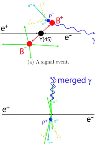
The most striking signature of a B → (ρ/ω) γ decay is the presence of a very high-energy photon in the event. In the system of the B meson decaying into the signal mode, the photon energy is about half the B meson mass. This still holds for the center of momentum (CM) frame of the whole event since the B mesons have only a momentum of 341 MeV/c in the CM frame. In each event, the highest energy photon is selected and required to have an energy between 1.5 GeV and 3.5 GeV in the CM frame. In the reconstruction, a photon is identified as a cluster in the electromagnetic calorimeter with no associated charged track.
Also, the event has to contain at least one well-reconstructed charged track which is identified as a pion. The excellent charged particle identification capabilities of the
BABAR detector is very useful for this purpose. The most important information for
pion identification is provided by the DIRC and supplemented by the measurement of dE/dx from the DCH and SVT.
The last type of particle needed to be able to reconstruct the signal B meson is a
π0, except for the decay mode B0 → ρ0γ. π0 candidates are identified by computing
the invariant mass of all pairs of photons in the event (which have to fulfill some quality requirements) and requiring that the computed invariant mass of this photon pair be close to the nominal π0 mass of (134.9766 ± 0.0006) MeV/c2 [22].
3.3
Major Backgrounds
The major background for this analysis originates from e+e−→ q ¯q events (where q =
can be mimicked in the following ways:
• The process e+e− → q ¯qγ can occur due to initial state radiation (ISR) or final
state radiation. In particular, a photon due to ISR can have very high energy and thus fake a photon from a signal event.
• The high-energy photon can be a decay product of a high-energy π0(η). This
high-energy π0(η) can decay into a photon pair with very asymmetric energies
in the lab frame and the low-energy photon can be lost, e.g. by going along the beam pipe. Or the two photons from the high-energy π0(η) can be in the same
cluster in the calorimeter and thus be identified as only one photon.
Due to the jetlike structure of these so-called continuum events, the high-energy photon is highly correlated with the energy and momentum flow of the rest of the event. This is not the case for an isotropic signal event since the B mesons have only a momentum of about 341 MeV/c in the CM frame.
Potentially dangerous are so-called “peaking backgrounds”. These are real B meson events that decay into a mode very similar to the true signal, e.g., B → K∗γ,
K∗ → Kπ where the kaon was mis-identified as a pion.
3.4
Expected Yields
In the 316 fb−1 of data used for this analysis, one expects about 350, 175, and 175 signal events produced in the channels B+ → ρ+γ, B0 → ρ0γ, and B0 → ωγ,
respectively. The expected number of potentially reconstructed signal events is further reduced due to the branching fraction of the ω → π+π−π0 decay of (89.1 ± 0.7) %
[22], the branching fraction of the π0 → γγ decay of (98.798 ± 0.032) % [22] and the
detector hermeticity of about 90%. Ignoring angular correlations and momentum distributions, one expects about 70% of the initial B+ → ρ+γ candidates to be
found in the detector, 75% of the initial B0 → ρ0γ candidates and about 60% of the
B
-B
+
Y(4S)
e-
γ
e
+
ρ
+ π0 γ γ π+(a) A signal event.
merged γ
e-e
+
ρ
+ π0 γ γ π+ π0(b) A continuum background event with a high energy π0.
γ
e-e
+
ρ
+ π0 γ γ π+(c) A continuum background event with ISR.
Also, w.r.t. the previous BABAR analysis on B → (ρ/ω) γ [24], the continuum
background suppression is expected to be improved due to an intended increase in the high-energy photon purity, a use of more signal-background separating variables in a higher-dimension neural network and a set of newly optimized cuts.
3.5
A Blind Analysis
This analysis is done “blind”, which means that all the analysis optimizations and considerations are based on so called MC simulations The real data is looked at only after the whole analysis procedure is fixed. The continuum MC can be verified with off–resonance data. This data has been collected in a mode where the collision energy
√
s is reduced by 40 MeV. It is sufficiently away from the Υ(4S) resonance so that
no B mesons can be produced.
In MC events the type of a generated particle is known. This MC truth information is used to optimize the analysis with respect to the efficiency of the true signal events, referred to as truth matched MC hereafter.
3.6
Data Samples
3.6.1
Monte Carlo
In this analysis, Monte Carlo simulations have been used to optimize the different selection criteria of the analysis. They are referred to as SP8 Monte Carlo or simply MC in the remainder of this thesis. There are several categories of MC:
• First, there is so-called signal MC which simulates e+e− → Υ(4S) → BB
where one B meson is constrained to decay into only a specific decay mode under consideration, e.g. B0 → ρ0γ, but the other B meson in the event is
allowed to decay generically into all final states. This type of MC is available in rather large amount, in terms of equivalent integrated data luminosity, due to the usually small branching fraction of the considered specific B decay.
Decay Branching Fraction (in 10−6) Generated Events Corresponding Luminosity (fb−1) B+ → ρ±γ 1 280000 266667 B0 → ρ0γ 0.5 328000 312381 B0 → ωγ 0.5 328000 312381 B0 → K∗0γ 39.2 ± 3.1 2155000 52357 B+ → K∗+γ 38.7 ± 3.8 2019000 49682 B0 → X0 sdγ 352 434000 1233 B+ → X+ suγ 352 434000 1233
Table 3.1: Signal Monte Carlo modes used in this analysis. The assumed cross section for the process e+e− → Υ(4S) → BB is 1.05nb [26].
Decay Assumed cross section (nb) [26] Generated Events Corresponding Luminosity (fb−1) e+e−→ Υ(4S) → B0B0 0.525 428558000 816.301 e+e−→ Υ(4S) → B+B− 0.525 416022000 792.423 e+e−→ uu, dd, ss 2.09 535274000 256.112 e+e−→ cc 1.30 497006000 382.311 e+e−→ τ+τ− 0.94 272228000 289.606
Table 3.2: Generic Monte Carlo modes used in this analysis.
• Second, there is so-called generic B MC. Here, the generic process e+e− →
Υ(4S) → BB is simulated and both B mesons in the event are allowed to decay into all possible final states. This type of MC is available in amount of about a few times the equivalent integrated data luminosity.
• Last, but not least, there is the so-called continuum MC. This is the simulation
of non-resonant physics processes under the Υ(4S) peak, i.e. e+e−→ f f , where
f is a either a quark lighter than the b quark (u, d, s, c) or a charged lepton.
Due to the large cross-section of these processes the available MC is usually only about one times the equivalent integrated data luminosity.
The MC samples used in this analysis are listed in Table 3.1 and Table 3.2 for signal MC and the generic B and continuum MC, respectively.

![Figure 2-9: The B A B AR Instrumented Flux Return [27].](https://thumb-eu.123doks.com/thumbv2/123doknet/14140015.470258/37.918.143.775.113.455/figure-b-b-ar-instrumented-flux-return.webp)
![Table 3.1: Signal Monte Carlo modes used in this analysis. The assumed cross section for the process e + e − → Υ(4S) → BB is 1.05nb [26].](https://thumb-eu.123doks.com/thumbv2/123doknet/14140015.470258/47.918.236.686.106.330/table-signal-monte-carlo-analysis-assumed-section-process.webp)