Experimental study of the structure and dynamics of cavitating flows

(1)

HAL Id: tel-03130085

https://pastel.archives-ouvertes.fr/tel-03130085

Submitted on 3 Feb 2021

HAL is a multi-disciplinary open access archive for the deposit and dissemination of sci-entific research documents, whether they are pub-lished or not. The documents may come from teaching and research institutions in France or abroad, or from public or private research centers.

L’archive ouverte pluridisciplinaire HAL, est destinée au dépôt et à la diffusion de documents scientifiques de niveau recherche, publiés ou non, émanant des établissements d’enseignement et de recherche français ou étrangers, des laboratoires publics ou privés.

Experimental study of the structure and dynamics of

cavitating flows

Guangjian Zhang

To cite this version:

Guangjian Zhang. Experimental study of the structure and dynamics of cavitating flows. Electric power. HESAM Université, 2020. English. �NNT : 2020HESAE050�. �tel-03130085�

(2)

[Laboratoire de Mécanique des Fluides de Lille – Campus de Lille]

THÈSE

présentée par :

Guangjian ZHANG

soutenue le : 2 Décembre 2020

pour obtenir le grade de :

Docteur d’HESAM Université

préparée à :

École Nationale Supérieure d’Arts et Métiers

Spécialité : Génie énergétique

Etude expérimentale de la structure et de la

dynamique des écoulements cavitants

THÈSE dirigée par :

[M. COUTIER-DELGOSHA Olivier]

Jury

M. Todd LOWE, Professeur, Virginia Tech Président M. Antoine DUCOIN, Maître de Conférences HDR, Ecole Centrale de Nantes Rapporteur M. Lionel THOMAS, Maître de conférences HDR, Université de Poitiers Rapporteur M. Joseph KATZ, Professeur, Johns Hopkins University Examinateur M. Matevž DULAR, Professeur, University of Ljubljana Examinateur M. Nathanaël MACHICOANE, Maître de conférences, Examinateur Université Grenoble Alpes

M. Olivier COUTIER-DELGOSHA, Professeur, Examinateur Arts et Métiers Sciences et Technologies

T

H

È

S

E

(3)

(4)

Acknowledgements

First of all, I would like to express my deepest gratitude to my supervisor Prof. Olivier Coutier-Delgosha for providing me the opportunity to pursue my PhD in his group. His continuous guidance and critical comments have improved this thesis work substantially. His work enthusiasm inspired me to never give up even though with huge frustrations.

I would also like to thank my committee members including Prof. Todd Lowe (Virginia Tech), Prof. Antoine Ducoin (Ecole Centrale de Nantes), Prof. Lionel Thomas (Université de Poitiers), Prof. Joseph Katz (Johns Hopkins University), Prof. Matevž Dular (University of Ljubljana) and Prof. Nathanaël Machicoane (Université Grenoble Alpes) for reviewing my thesis and providing me valuable suggestions.

Sincere thanks are given to Prof. Antoine Dazin and Prof. Annie-Claude Bayeul-Laine for being in my academic follow-up committee. Their rich experience and knowledge always guide me to work in the right direction.

The X-ray imaging experiment was performed at the Advanced Photon Source, and many thanks to Dr. Kamel Fezzaa for his kind help with our experimental setup. I am grateful to Dr. Ilyass Khlifa for his guidance to develop the image-processing method to separate particles from raw X-ray images. I would like to thank my friend, roommate as well as colleague Dr. Xinlei Zhang for his help both in work and life.

The PIV-LIF measurements of cavitating flows were carried out in the Cavitation, Propulsion & Multiphase Flow Laboratory of Virginia Tech. I would like to thank Mr. Mingming Ge, Mr. Navid Nematikourabbasloo and Dr. Merouane Hamdi for aiding me to complete this experiment.

I had an opportunity of visiting Virginia Tech for a number of months. I am grateful to Dr. Zhongshu Ren, Mr. Ben Zhao, Mr. Yuzhi Li and Mr. Mingming Ge for helping me adapt to the new environment quickly. Because of you guys, we managed to go hiking, have hot-pot and visit a lot of interesting places. You guys make my stay in Virginia Tech exciting and memorable.

(5)

My sincere appreciation extends to all colleagues at the ENSAM for their help in my work and life, especially to Mr.Alberto Baretter, Mr. Lei Shi, Dr. Yuxin Bai, Mr.Kunpeng Long, Mrs. Naly Ratolojanahary and Mr. Mohamed Ghandour.

Finally and most importantly, I would like to thank my parents for their limitless love and support during my life time. I would also like to thank my girlfriend LR to accompany me in the past 12 years.

(6)

I

List of Symbols

Latin

𝑓 Frequency, [Hz]

ℎ_te Height at the test section entrance, [m]

ℎ_th Height at the Venturi throat, [m]

ℎve Height at the Venturi entrance, [m]

𝐼_𝛼 Local image intensity with cavitation

𝐼₀ Local image intensity with vapor

𝐼₁ Local image intensity with water

𝑘 Turbulent kinetic energy, [m2_/s2_]

𝐿cav Mean cavity length, [m]

𝑃_in Static pressure at the inlet, [Pa]

𝑃_out Static pressure at the outlet, [Pa]

𝑃_in′∗ Nondimensional pressure fluctuations at the inlet 𝑃_out′∗ Nondimensional pressure fluctuations at the outlet

𝑃_vap Saturated vapor pressure, [Pa]

𝑄 Volumetric flow rate, [m3/s]

𝑅₁ Source to object distance, [m]

𝑅₂ Object to detector distance, [m]

𝑆𝑡 Strouhal number

𝑡 Time, [s]

𝑇_cav Mean cavity thickness, [m]

𝑢 Longitudinal velocity, [m/s]

𝑢 Mean longitudinal velocity, [m/s]

𝑢′ Longitudinal velocity fluctuation, [m/s]

(10)

V

𝑢_ref Average velocity at the Venturi throat 𝑢_thas a reference, [m/s]

𝑢re Re-entrant jet velocity, [m/s]

𝑢sh Propagation speed of the condensation shock, [m/s]

𝑢_wa Travelling velocity of the pressure wave, [m/s]

𝑣′ _{Transversal velocity fluctuation, [m/s]}

𝑥 First Cartesian coordinate, [m]

𝑦 Second Cartesian coordinate, [m]

𝑧 Third Cartesian coordinate, [m]

Greek

𝜎 Inlet cavitation number

𝜌 Liquid/vapor mixture density, [kg/m3]

𝜌𝑙 Liquid density, [kg/m3]

𝜌𝑣 Vapor density, [kg/m3]

𝛼 Vapor volume fraction, i.e. void fraction

𝛼 Mean void fraction

𝛼′ Standard deviation of void fraction

𝜏 Reynolds shear stress, [m2_/s2_]

Acronyms

APS Advanced Photon Source

CCD Charge Coupled Device

CT Computed Tomography

FFT Fast Fourier Transform

LES Large Eddy Simulation

LIF Laser-Induced Fluorescent

PDF Probability Density Function

PIV Particle Image Velocimetry

(11)

(12)

1

Chapter 1 Introduction

1.1. Introduction to cavitation phenomenon

Cavitation is a unique phase change phenomenon in liquid flows involving processes of the explosive vaporization of liquid in low pressure regions and the subsequent implosions when the pressure increases again. In contrast to boiling where the vaporization of liquid is driven by a temperature change, cavitation could be approximated as an isothermal process starting when the local liquid pressure is reduced below its saturated vapour pressure. Moreover, cavitation inception is also subjected to cavitation nuclei like non-condensable gases or other pollutants in liquid. Their existence weakens cohesion of liquid molecules and thus serves as starting locations for the liquid breakdown with decreasing the ambient pressure. The cavitation nuclei content is also a primary factor determining the difference between the vapour pressure and the actual pressure at cavitation inception (Franc & Michel 2005).

Cavitation can be classified, according to generation mechanisms, into acoustic cavitation, laser-induced cavitation and hydraulic cavitation. The first two types are produced through either ultrasonic waves or lasers depositing high amounts of energy into the liquid locally. The last one is caused by low pressures associated with flow dynamics, such as flow accelerations and strong vortical motions. In the literature and also in the present thesis, cavitation, if there is no specific note, usually refers to hydraulic cavitation since it is the most common and important case encountered in engineering applications.

Hydraulic cavitation can take different forms depending on how the low-pressure regions are generated, and they can be divided into three groups:

⚫ Travelling bubble cavitation. Individual bubbles arise from regions of cavitation inception as a result of rapid growth of cavitation nuclei. They are first transported by the flow and then implode when they reach zones of high pressure.

(13)

2

⚫ Attached cavitation. It appears in a low-pressure separated region close to the solid surface. The typical flow scenarios are cavities forming on the suction side of a hydrofoil or an impeller blade. If the length of the attached cavity exceeds the body upon which it develops, it is called super cavitation, otherwise it is termed as partial cavitation.

⚫ Vortex cavitation. The fluid in the cores of vortices is prone to vaporizing due to low pressures prevailing there. It is commonly observed at the tips of propeller blades or in the free shear layers where Kelvin-Helmholtz vortices can develop.

In most hydraulic applications like turbo-machinery and marine propellers, cavitation is an undesired phenomenon, since the unsteady behavior and violent collapse of cavitation can result in detrimental effects, such as noise, system vibrations, performance decrease, material erosion, etc. However, in some cases, cavitation can have positive consequences. For instance, the torpedoes are enveloped in a stable super-cavity for reducing frictions with water, so that they are able to reach very high speeds (about 400 km/h). The intensive energy released from a collapsing cavity could be utilized to destroy kidney stones for treatment or kill live bacteria for cleaning of waste water.

Although cavitation has been investigated extensively for more than a century, a full understanding of the physical processes underlying the cavitating flows is still far from being realized at the present time.This is mainly due to the lack of quantitative experimental data on two-phase structures and dynamics of cavitation. Therefore, high-fidelity and detailed measurements of cavitating flow fields, especially in the opaque diphasic mixture areas, are extremely desired for a better knowledge of the physical mechanisms governing the cavitation instabilities. This will help to deduce effective means for controlling the negative consequences of cavitation and increasing its positive influence. Furthermore, the quantitative experimental data can be used to validate and improve the numerical simulation models for cavitation. Once reliable predictions are achieved, the costs and time concerning cavitation tests will be reduced substantially.

1.2. Outline of the thesis

Following the previous works in our group (Coutier-Delgosha et al. 2009; Khlifa et al. 2017), partial cavitation developed in small convergent-divergent (Venturi) channels were studied experimentally using an ultra-fast synchrotron X-ray imaging technique aided with

(14)

3

conventional high speed photography as well as particle image velocimetry (PIV). Depending on different operating conditions and geometry dimensions, partial cavitation generally exhibited two regimes with distinct behaviors: quasi-stable sheet cavitation and periodic cloud cavitation with large vapour shedding. The measurement results in the present study provided a detailed description of the two-phase flow structures and dynamics in sheet cavitation. Three mechanisms responsible for the transition of sheet-to-cloud cavitation were revealed and the differences between them were highlighted.

This thesis is composed of the following 7 chapters. Chapter 2 is a literature review on the physical background of sheet/cloud cavitation and the existing experimental techniques applied to cavitating flows. Chapter 3 provides a brief description of the experimental setup and the fast X-ray imaging technique. The emphasis of this chapter is put on the procedures from visualizations to velocity and void fraction field measurements in cavitating flows.In Chapter 4, the complex two-phase flow structures inside the sheet cavity are revealed in detailbased on the data from the X-ray measurements. Chapter 5 deals with a comparative study of sheet cavitation at three stages (the early stage, intermediate stage and developed stage). The comparison shows the effect of re-entrant jet behaviors on sheet cavity structures and dynamics. The influence of cavitation on turbulent fluctuations is also discussed. Chapter 6 analyzes the cavitating flows in a Venturi channel with side gaps. It is found that cloud cavitation can be suppressed by altering the propagation path of the re-entrant jet. In Chapter 7, three mechanisms (i.e. re-entrant jet mechanism, condensation shock mechanism and collapse-induced pressure wave mechanism) to initiate cloud cavitation are described in detail, and the reasons causing the scale effect on Venturi cavitating flows are discussed. The thesis is ended with ageneral conclusion in Chapter 8 summarizing the main contributions of this work and several perspectives for future research are proposed.

1.1. Introduction au phénomène de cavitation

La cavitation est un phénomène de changement de phase unique dans les écoulements de liquide impliquant des processus de vaporisation explosive de liquide dans les régions à basse pression et les implosions ultérieures lorsque la pression augmente à nouveau. Contrairement à l'ébullition où la vaporisation du liquide est entraînée par un changement de température, la cavitation pourrait être approchée comme un processus isotherme commençant lorsque la

(15)

4

pression locale du liquide est réduite en dessous de sa pression de vapeur saturée. De plus, l'amorce de la cavitation est également soumise à des noyaux de cavitation comme des gaz non condensables ou d'autres polluants dans le liquide. Leur existence affaiblit la cohésion des molécules liquides et sert ainsi de points de départ pour la dégradation du liquide avec diminution de la pression ambiante. Le contenu des noyaux de cavitation est également un facteur principal déterminant la différence entre la pression de vapeur et la pression réelle au début de la cavitation (Franc & Michel 2005).

La cavitation peut être classée, selon les mécanismes de génération, en cavitation acoustique, cavitation induite par laser et cavitation hydraulique. Les deux premiers types sont produits soit par des ondes ultrasonores, soit par des lasers déposant localement de grandes quantités d'énergie dans le liquide. Le dernier est causé par les basses pressions associées à la dynamique de l'écoulement, telles que les accélérations de l'écoulement et les forts mouvements tourbillonnaires. Dans la littérature comme dans la présente thèse, la cavitation, s'il n'y a pas de note spécifique, fait généralement référence à la cavitation hydraulique car c'est le cas le plus courant et le plus important rencontré dans les applications d'ingénierie.

La cavitation hydraulique peut prendre différentes formes selon la façon dont les régions à basse pression sont générées, et elles peuvent être divisées en trois groupes:

⚫ Cavitation à bulles itinérantes. Les bulles individuelles proviennent de régions de début de cavitation suite à la croissance rapide des noyaux de cavitation. Ils sont d'abord transportés par le flux puis implosent lorsqu'ils atteignent des zones de haute pression.

⚫ Cavitation attachée. Il apparaît dans une région séparée par basse pression proche de la surface solide. Les scénarios d'écoulement typiques sont des cavités se formant du côté aspiration d'un hydroptère ou d'une aube de turbine. Si la longueur de la cavité attachée dépasse le corps sur lequel elle se développe, on parle de super cavitation, sinon on parle de cavitation partielle.

⚫ Cavitation vortex. Le fluide dans les noyaux des tourbillons a tendance à se vaporiser en raison des basses pressions qui y règnent. Il est couramment observé aux extrémités des pales d'hélices ou dans les couches de cisaillement libre où peuvent se développer des tourbillons de Kelvin-Helmholtz.

Dans la plupart des applications hydrauliques comme les turbomachines et les hélices marines, la cavitation est un phénomène indésirable, car le comportement instable et l'effondrement violent de la cavitation peuvent entraîner des effets néfastes, tels que le bruit,

(16)

5

les vibrations du système, la diminution des performances, l'érosion des matériaux, etc. dans certains cas, la cavitation peut avoir des conséquences positives. Par exemple, les torpilles sont enveloppées dans une super-cavité stable pour réduire les frottements avec l'eau, afin qu'elles puissent atteindre des vitesses très élevées (environ 400 km/h). L'énergie intensive libérée par une cavité qui s'effondre pourrait être utilisée pour détruire les calculs rénaux pour le traitement ou pour tuer les bactéries vivantes pour le nettoyage des eaux usées.

Bien que la cavitation ait été largement étudiée depuis plus d'un siècle, une compréhension complète des processus physiques sous-jacents aux écoulements de cavitation est encore loin d'être réalisée à l'heure actuelle. Ceci est principalement dû au manque de données expérimentales quantitatives sur les structures biphasées et la dynamique de la cavitation. Par conséquent, des mesures haute fidélité et détaillées des champs d'écoulement de cavitation, notamment dans les zones de mélange diphasique opaque, sont extrêmement recherchées pour une meilleure connaissance des mécanismes physiques régissant les instabilités de cavitation. Cela permettra de déduire des moyens efficaces pour contrôler les conséquences négatives de la cavitation et augmenter son influence positive. De plus, les données expérimentales quantitatives peuvent être utilisées pour valider et améliorer les modèles de simulation numérique pour la cavitation. Une fois que des prévisions fiables sont réalisées, les coûts et le temps relatifs aux essais de cavitation seront considérablement réduits.

1.2. Aperçu de la thèse

Suite aux travaux précédents de notre groupe (Coutier-Delgosha et al.2009; Khlifa et al.2017), la cavitation partielle développée dans de petits canaux convergents-divergents (Venturi) a été étudiée expérimentalement à l'aide d'une technique d'imagerie par rayons X synchrotron ultra-rapide assistée. avec la photographie conventionnelle à grande vitesse ainsi que la vélocimétrie d'image de particules (PIV). En fonction des conditions de fonctionnement et des dimensions géométriques différentes, la cavitation partielle présentait généralement deux régimes avec des comportements distincts: la cavitation en nappe quasi-stable et la cavitation nuageuse périodique avec une grande évacuation de vapeur. Les résultats de la mesure dans la présente étude ont fourni une description détaillée des structures et de la dynamique de l'écoulement diphasique dans la cavitation en feuille. Trois mécanismes responsables de la transition de la cavitation feuille à nuage ont été mis en évidence et les différences entre eux ont été mises en évidence.

(17)

6

Cette thèse est composée des 7 chapitres suivants. Le chapitre 2 est une revue de la littérature sur le contexte physique de la cavitation en nappe / nuage et les techniques expérimentales existantes appliquées aux écoulements de cavitation. Le chapitre 3 fournit une brève description de la configuration expérimentale et de la technique d'imagerie rapide par rayons X. L'accent de ce chapitre est mis sur les procédures allant des visualisations aux mesures de vitesse et de champ de fraction de vide dans les écoulements de cavitation. Dans le chapitre 4, les structures d'écoulement diphasiques complexes à l'intérieur de la cavité de la feuille sont révélées en détail sur la base des données des mesures aux rayons X. Le chapitre 5 traite d'une étude comparative de la cavitation des plaques à trois stades (stade précoce, stade intermédiaire et stade développé). La comparaison montre l'effet des comportements des jets rentrants sur les structures et la dynamique des cavités de la feuille. L'influence de la cavitation sur les fluctuations turbulentes est également discutée. Le chapitre 6 analyse les écoulements de cavitation dans un canal Venturi avec des espaces latéraux. On constate que la cavitation des nuages peut être supprimée en modifiant le trajet de propagation du jet rentrant. Dans le chapitre 7, trois mécanismes (à savoir le mécanisme de jet rentrant, le mécanisme de choc de condensation et le mécanisme d'onde de pression induite par l'effondrement) pour initier la cavitation des nuages sont décrits en détail, et les raisons provoquant l'effet d'échelle sur les écoulements de cavitation Venturi sont discutées. La thèse se termine par une conclusion générale au chapitre 8 résumant les principales contributions de ce travail et plusieurs perspectives de recherches futures sont proposées.

(18)

7

Chapter 2 Physical background and measurement techniques

2.1. Sheet and cloud cavitation

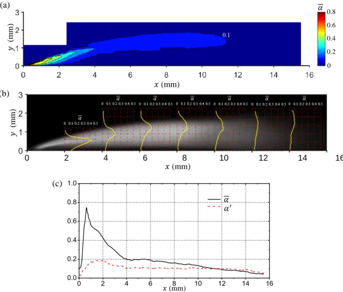
Generally speaking, partial cavities have two forms of appearance as well in case of internal flows (in a Venturi) as in case of external flows (on a hydrofoil).For small incident angles (hydrofoil – angle of attack; Venturi – divergent and convergent angles) and high free-stream cavitation numbers, the attached cavity appears to be stationary at a fixed location, and the observed cavity length is rather constant. This situation is referred to as sheet cavitation. A typical sheet cavitation forming on the suction side of a hydrofoil or on the divergent wall of a Venturi channel is presented in Figure 2.1. When the cavitation number is decreased or/and the incident angle is increased to a certain extent, the stable sheet cavity cannot be sustained. A large portion of the cavity is shed periodically from the main cavity forming a cloud-like structure in the cavity wake, and as a result the cavity length undergoes significant oscillations. This phenomenon is commonly called cloud cavitation. Figure 2.2 shows two examples of cloud shedding.

Although cavitation is inherently unsteady, sheet cavitation is usually stated to be stable or quasi-stable since the shedding of small vapour-filled vortices is confined in the cavity closure region, whose characteristic length scale is much smaller than the whole cavity length. Sheet cavitation is sometimes described to be an open cavity due to its frothy appearance at the closure as classified by Laberteaux & Ceccio (2001a). In contrast, cloud cavitation results in large fluctuations of cavity volume and thus is stated to be unstable. The violent collapse of the shed cloud in the downstream wake region can emit pressure waves of high amplitude, which is considered as the main source of noise and erosion (Reisman et al. 1998; Dular et al. 2015). Therefore, cloud cavitation is much more destructive than a stable sheet cavity.

(19)

8

Figure 2.1. (a) Sheet cavitation on the suction side of a hydrofoil from Foeth (2008b); (b) sheet cavitation on the divergent wall of a Venturi channel from Barre et al. (2009).

Figure 2.2. (a) Cloud cavitation on the suction side of a hydrofoil from Foeth (2008b); (b) cloud cavitation on the divergent wall of a Venturi channel from Stutz &Reboud (1997a).

2.2. Mechanisms for cloud shedding

In a classical point of view, the different behaviors of a partial cavity depend on the existence or absence of re-entrant flow originating from a stagnation point behind the cavity closure.

As for sheet cavitation (open partial cavities), Gopalan & Katz (2000), Callenaere et al. (2001) and Laberteaux & Ceccio (2001a) concluded that no clear re-entrant jet or only the weak reverse flow existed at the trailing edge of the cavity due to weak adverse pressure gradient. Leroux et al. (2004) did not detect a clear sign of a pressure wave traveling from the cavity closure towards the leading edge inside a stable sheet cavity through ten aligned pressure transducers flush-mounted along the suction side of a hydrofoil, and they attributed it to the absence of the re-entrant jet. Barre et al. (2009) measured a clear re-entrant flow in a globally-steady sheet cavitation using a double optical probe technique. However, in their simultaneous numerical simulation, the re-entrant jet was not predicted, and eventually they did not further clarify the role played by the re-entrant jet in stable sheet cavitation. In general, the absence of re-entrant flow was regarded as the main reason for the stable flow regime of sheet cavitation. The periodic shedding of large cloud was observed firstly by Knapp (1955) and he proposed a re-entrant jet model to explain the transition from stable sheet cavitation to periodic

(a) (b)

(20)

9

cloud cavitation.This re-entrant jet mechanism is presented schematically in Figure 2.3. As the attached cavity grows to a certain length, a thin re-entrant jet, mainly composed of liquid, forms near the cavity closure region and moves upstream beneath the cavity. When this jet reaches the cavity leading edge, the whole cavity is pinched off forming a rolling cavitation cloud that is then convected downstream by the main flow until it collapses. Meanwhile a new cavity begins to grow again and the entire process is repeated.

Figure 2.3. Typical unsteady behavior of a partial cavity with the development of a re-entrant jet and the periodic shedding of cavitation clouds from Franc & Michel (2005).

After the establishment of the re-entrant jet model, many studies have been conducted in order to verify the existence, development, the correlation of re-entrant jet with cavitation dynamics. Furness & Hutton (1975) predicted the development of re-entrant jet using a potential flow model. The injection of ink was used by Le et al. (1993) to visualize the re-entrant flow, and the ink was observed near the leading edge, confirming an upstream flow component. Kawanami et al. (1997) placed a small obstacle on the suction side of a hydrofoil to prevent the re-entrant jet from moving upstream, and the large cloud shedding was not observed in the experiment, demonstrating the re-entrant jet was the primary cause of cloud cavitation. Pham et al. (1999) placed a series of six electrical impedance probes spaced equally on the upper flat surface of the hydrofoil to detect the liquid front corresponding to the re-entrant jet. They found that the mean velocity of the re-re-entrant jet attained a maximum value

(21)

10

near the cavity closure region and was of the same order of magnitude as the free stream velocity. Laberteaux & Ceccio (2001b) observed that a geometry with spanwise variation can sustain stable cavities with re-entrant flow since the re-entrant flow was directed away from the cavity. The conditions necessary for the development of the re-entrant jet has been explored by Callenaere et al. (2001). They confirmed the critical role of the adverse pressure gradient at the cavity closure in the onset of the re-entrant jet instability.

In the numerical simulation of cloud cavitation, the RANS models generally overestimate the turbulent viscosity in the rear part of the cavity. The re-entrant jet is consequently stopped too early and it does not result in any cavity break off. Coutier-Delgosha et al. (2003) reproduced the periodic cloud shedding in a Venturi-type section by using a correction initially proposed in Reboud et al. (1998) on turbulent viscosity which actually reduces the friction losses that the re-entrant jet encounters. Pelz et al. (2017) introduced a physical model of transition from sheet to cloud cavitation based on the criterion that the transition occurs when the re-entrant jet reaches the point of origin of the sheet cavity. A good agreement was found between the model-based calculations and the experimental measurements. Their numerical work could also demonstrate the importance of re-entrant jet to initiate cloud cavitation.

Figure 2.4. Instantaneous void fraction fields illustrating the condensation shock mechanism to cause sheet-to-cloud cavitation from Ganesh et al. (2016).

In addition to the classical re-entrant jet, the mechanism of condensation shock waves dictating sheet-to-cloud shedding has been widely acknowledged in recent years. As early as

(22)

11

1964, the occurrence of condensation shocks in cavitating flows was speculated by Jakobsen (1964) based on the fact that the sound speed in a two-phase mixture is significantly lower than that in either component, i.e. water or water vapour (Brennen 1995). However, the direct experimental observation was made only recently by Ganesh et al. (2016). As shown in Figure 2.4, using X-ray densitometry to visualize the instantaneous distribution of vapour volume fraction in the cavitating flow over a wedge, they found that the leading edge cloud shedding at lower cavitation numbers was resulted from an upstream propagating void fraction discontinuity, i.e. a condensation shock front. In order to demonstrate this new finding different from the classical re-entrant jet mechanism, Ganesh et al. (2017) also placed a small obstacle under the sheet cavity just like what Kawanami et al. (1997) did. The results showed that cloud shedding in the case of condensation shocks cannot be prevented since the condensation front spans the entire cavity height rather than near the wall only.

Motivated by the pioneering work of Ganesh et al. (2016), many interesting numerical and experimental studies were performed later towards revealing the condensation shock mechanism in different configurations (e.g. Wu et al. 2017; Jahangir et al. 2018; Budich et al. 2018; Wu et al. 2019; Trummler et al. 2020; Bhatt & Mahesh 2020). In agreement with the original experiment, all these works found that with a sufficient reduction of the cavitation number, condensation shocks overtaking re-entrant jets became the dominant mechanism for large-scale cloud shedding. Nevertheless, they had divergence on the cause for the onset of condensation shock. In the PhD thesis of Ganesh (2015), it was described that a rapid growth in cavity length and vapour content, hence reduced speed of sound and increased compressibility, resulted in the production of shock waves at the rear of the cavity. Wu et al. (2017), Jahangir et al. (2018) and Bhatt & Mahesh (2020) observed that the propagation of condensation shocks was triggered by the impingement of collapse-induced pressure waves from previously shed clouds. This was also found by Budich et al. (2018), but in addition they also captured the initiation of condensation shocks in the absence of cloud collapsing. It implied that both the rapid cavity growth and the collapse-induced pressure wave could contribute to the formation of overpressure behind the cavity which was sufficient to induce a condensation shock front. It should be noted that a pressure wave with high amplitude emanating from a large cloud collapse might crush the growing cavity suddenly as described by Leroux et al. (2005), which was different from the propagation of condensation shock through the cavity.

(23)

12 2.3. Studies on cavitation-turbulence interactions

The cavitation dynamics is also strongly related to the cavitation / turbulence coupling: the effect of cavitation (including formation and collapse of vapour cavities) on turbulence has been investigated numerically and experimentally.

As for the numerical aspect, Dittakavi et al. (2010) used large eddy simulation (LES) to predict cavitating flows in a Venturi nozzle. By comparison of three cases at different cavitation numbers, they concluded that the vapour formation due to cavitation suppressed turbulent velocity fluctuations and the collapse of vapour structures in the downstream region was a major source of vorticity production, resulting in a substantial increase of turbulent kinetic energy. Xing et al. (2005) observed, in their numerical simulation of vortex cavitation in a submerged jet, that cavitation suppressed jet growth and decreased velocity fluctuations within the vaporous regions of the jet. Gnanaskandan & Mahesh (2016) investigated partial cavitating flows over a wedge and found that the streamwise velocity fluctuations dominated the other two components within the cavity, while all three components of fluctuations were equally significantnear the cavity closure and downstream of the cavity,

Regarding the experimental aspect, the acquisition of quantitative velocity fields mainly relied on PIV measurements. Gopalan & Katz (2000) and Laberteaux & Ceccio (2001) observed the largest turbulent fluctuations in the region downstream of the cavity which were regarded as the impact of vapour collapse. Iyer & Ceccio (2002) investigated the effect of developed cavitation on the flow downstream of the cavitating shear layer. They found that the collapse of vapour bubbles led the streamwise velocity fluctuations to be increased but the cross-stream fluctuations and the Reynolds shear stress to be decreased. Aeschlimann et al. (2011b) performed velocity measurements in a 2D cavitating shear layer. They observed that a complex combination of the production of vapour bubbles coupled with their collapse added additional velocity fluctuations, mostly in the main flow direction, while the turbulent shear stresses almost remained constant.

2.4. A review of measurement techniques for cavitating flows

Detailed flow measurements are essential for the understanding of cavitating flows. Due to the existence of non-transparent liquid/vapour mixtures, visual observation by a fast speed camera (high speed photography) is the most straightforward and widely-used method to capture the temporal evolution of cavitation structures, thereby providing insight into the underlying physics (Foeth et al. 2008a; Aeschlimann et al. 2012). Through post-processing of

(24)

13

the high speed video images, it is possible to derive some quantitative data, such as the cloud shedding frequency and the cavity growth rate (Prothin et al. 2016; Jahangir et al. 2018). Synchronized with dynamic pressure measurements, high speed images can also reveal the pressure change associated with the cavity unsteady behaviors (Wang et al. 2017; Wu et al. 2017). On one hand, cavitation visibility helps to obtain its global flow characteristics. On the other hand, cavitation opacity hinders the measurements inside the two-phase region. In order to analyze the internal flow structures of cavitation, other techniques, able to visualize the two-phase morphology as well as measure quantitative data on void fraction and velocity, are required.

2.4.1. Local measurements by intrusive probes

Ceccio & Brennen (1991) detected individual vapour bubbles using a network of silver electrodes mounted on the surface of a hydrofoil, and thus acquired their velocities. Stutz & Reboud (1997a; 1997b; 2000) used a double optical probe to measure the time-averaged void fraction and vapour-phase velocity inside the cavity generated in a two-dimensional Venturi-type section. In this technique, the local velocity was estimated by the time interval of a bubble passing two probe tips successively and the local void fraction was defined as the ratio of the cumulated time of vapour phase at the tip of the probe to a given time of observation. In spite of a relative large measurement uncertainty of about 15%, their work gave a preliminary description of the two-phase flow structure inside a sheet cavity and confirmed the presence of a reverse flow along the solid surface. Coutier-Delgosha et al. (2006) made the first attempt to visualize the two-phase morphology inside the sheet cavity by means of a new endoscopic device. Based on the observation at different stations along the hydrofoil chord, they found that the internal structure close to the leading edge was characterized by large vapour bubbles with a similar critical size and then they were rapidly split into smaller bubbles downstream; most of the bubbles do not have a spherical shape.

2.4.2. Particle Image Velocimetry (PIV)

Different from intrusive and pointwise measurements using probes, PIV enables a whole-field acquisition of instantaneous velocity vectors with little perturbation on the flow. It has thus been applied to a wide range of fluid flows, but in cavitating flows, the strong scattering and reflection from the liquid/vapour mixture will obscure the scattering light from the

(25)

14

surrounding tracer particles. This contaminating effect on the PIV measurements can be avoided by injecting laser-induced fluorescent (LIF) particles which emit light with different wavelength from the laser. The reflected and scattered light, at the wavelength of the laser, is blocked by the optical filter mounted in front of the lens and only the light emitted by the particles is recorded by the camera. However, if there are many vapour bubbles passing between the laser sheet and the camera, the optical paths starting from the fluorescent particles will be deviated severely or blocked completely. As a consequence, most PIV-LIF measurements have focused on the liquid flow regions outside the cavity (Laberteaux & Ceccio 2001; Foeth et al. 2006; Kravtsova et al. 2014) or turbulent cavitating regions with low void fraction (Iyer & Ceccio 2002; Aeschlimann et al. 2011b). Interestingly, the work of Dular et al. (2005) shows that if the positionof the laser sheet was close enough to the observation window (~5 mm), the detected particles would be sufficient to evaluate the velocity field inside the sheet cavity. However, the measured velocity field is not representative since it is strongly subjected to the wall effects.

2.4.3. X-ray densitometry based on absorption contrast

Both X-rays and visible light are, in nature, part of the electromagnetic spectrum. However, due to having a much shorter wavelength than visible light, X-rays can penetrate most optically opaque media with weak interactions. This distinct advantage makes X-ray radiography a powerful method to visualize opaque multiphase flows (Heindel 2011).

For cavitating flows, X-ray radiography can be used to measure local void fraction, i.e. density because of the absorption difference between water and vapour. Stutz & Legoupil (2003) applied firstly the X-ray densitometry to cloud cavitation formed in a Venturi-type test section. They found that the mean void fraction varies regularly from 25% at the upstream end of the mean cavity to 10% in the downstream part. Coutier-Delgosha et al. (2007) performed void fraction measurements of cavitation on a plano-convex hydrofoil using the same X-ray attenuation device. They reported that the local mean vapour volume fraction does not exceed 35 % for small sheet cavities, and 60 % for the large ones. Another application of X-ray attenuation measurements can be found in Aeschlimann et al. (2011a) where the main vortex shedding frequency in a turbulent cavitating shear layer was estimated through spectral analysis of the void fraction signal. In recent works (Ganesh et al. 2016; Wu et al. 2019), time-resolved X-ray densitometry was used to measure the instantaneous distribution of void fraction in the

(26)

15

cavitating flow field. A well-defined void-fraction discontinuity spanning the thickness of the cavity was observed to propagate upstream. According to the authors, this discontinuity represented a bubbly shock front which was responsible for periodic shedding of large-scale vapour clouds.

A standard 2D X-ray densitometry system can only provide a projection of the sample’s density distribution in the direction of the X-ray beam.This means that the 3D flow information is collapsed onto a single 2D plane. As a remedy, the actual 3D spatial distribution can be retrieved using a tomographic reconstruction. The examples of using X-ray computed tomography (CT) to measure the radial distribution of void fraction in circular nozzle cavitating flows can be found in Bauer et al. (2018) and Jahangir et al. (2019).

2.4.4. X-ray velocimetry based on phase contrast

X-ray phase-contrast imaging enables clear visualization of boundaries between phases with different refractive index (Kastengren & Powell 2014).Aside from detailed illustration of two-phase morphology (Karathanassis et al. 2018), X-ray phase-contrast images can also be used to perform velocimetry by tracking either seeded particles or phase interfaces. Early applications of X-ray velocimetry are for solving the so-called optical access issue. For example, Lee & Kim (2003) employed a low-energy synchrotron X-ray beam instead of a laser sheet to illuminate the seeded particles in the flow in an opaque tube. The instantaneous velocity field was extracted by cross-correction similar to the conventional PIV analysis. For opaque flows with a very low speed (a few millimeters per second), they also developed a compact X-ray-based PIV system employing a medical X-ray tube as a light source (Lee et al. 2009).

For high speed fluid flows, a short exposure time is needed to freeze the fluid motion. The third-generation synchrotron radiation sources such as the advanced photon source (APS) at Argonne National Lab can produce a high-energy and coherent X-ray beam which satisfies the requirements of ultra-fast X-ray phase-contrast imaging. Im et al. (2007) used the APS X-ray source to greatly improve the particle image quality making single-particle tracking velocimetry possible in an optically opaque vessel. Wang et al. (2008) revealed for the first time the internal structures of high-speed (order of 60 m/s) optically dense sprays near the nozzle exit using the ultrafast APS X-ray phase-contrast imaging technique. The velocity fields were measured by tracking the movements of the phase enhanced liquid–gas boundaries. A

(27)

16

similar application of synchrotron X-ray phase-contrast imaging in fuel injector nozzles was presented by Moon (2016) for comparing the dynamic structure of biodiesel and conventional fuel sprays.

The first attempt to measure velocity field inside cavitating regions by means of fast X-ray image was described by Coutier-Delgosha et al. (2009). Later Khlifa et al. (2017) also used the similar method to measure high speed cavitating flows in a small size Venturi-type test section. In the experiment, the flows were seeded with silver-coated hollow glass sphere particles which were visualized clearly along with the bubbly structures of cavitation by combined effects of X-ray absorption and phase contrast enhancement. Cross-correlation algorithms were applied on the particles and the bubble structures to evaluate the liquid-phase and the vapor-phase velocities respectively. Furthermore, the distribution of vapour volume fraction was determined from X-ray absorption difference in vapour and liquid. Based on the experimental results, the presence of significant slip velocities between the liquid and vapour phase was demonstrated quantitatively for the first time. Their work laid a foundation for the present study on flow structures and dynamics inside sheet cavities.

(28)

17

Chapter 3 Fast X-ray imaging technique and quantitative data

extraction based on image post-processing

The time-resolved, whole-field measurements inside a partial cavity have always been challenging due to the opaqueness of the liquid/vapour mixture. The lack of experimental data on the internal two-phase flow structures and dynamics has been a major issue for the understanding of the cavitation physics and the validation of the numerical models. Motivated by solving this problem, our group has developed in the last 13 years an ultra-fast X-ray imaging technique applied to situations of cavitating flows in a 2D Venturi-type section. Such a technique enables to obtain by image processing i) the liquid velocity field (tracking the motion of the seeding particles), ii) the vapour velocity field (tracking the motion of the vapour bubbles), and ⅲ) the distribution of the vapor volume fraction (based on the difference of X-ray absorption in vapour and water). In this chapter, a brief description of the fast X-X-ray imaging technique will be given, and the emphasis will be put on the procedures to obtain the velocity and void fraction fields, from the flow visualizations.

3.1. Hydraulic test rig

The studied sheet cavitation is generated in a small size Venturi-type test section installed in a closed hydraulic loop designed by Coutier-Delgosha et al. (2009) as shown in Figure 3.1. During the experiments, the test loop is filled with water driven by a circulating pump. The flow rate measured by a turbine flow meter is regulated by a frequency inverter varying the pump rotation speed. A secondary recirculation loop is added to attain small flow rates while avoiding the pump operating in off-design conditions. Different extent of cavitation could be set properly by adjusting the pressure on the free surface of the tank with the aid of a vacuum

(29)

18

pump or a pressurizer. A heater combined with a cooling system is employed enabling the flow temperature to stabilize at a given value that is measured by a thermocouple located upstream of the test section.

Figure 3.1. Schematic of the cavitation tunnel.

Figure 3.2. (a) Profile of Venturi-type test section; the convergent-divergent channel is formed by the lower insert part (2) with the confinement of the top wall (3); flow direction is from left to right, (b) detailed dimensions of the convergent-divergent section (in mm).

The overall test section 30 cm long is presented in Figure 3.2. The lower part (2) is inserted into the bottom wall (1) forming the convergent-divergent flow channel with the confinement of the top wall (3). The Venturi has a rectangular cross section and is characterized by a convergent angle of 18° and a divergent angle of 8°. The width of the flow passage is 4 mm. The height hve at the Venturi entrance is 17 mm with hth = 15.34 mm at the throat producing a small contraction ratio of 1.1. The height hte of the test section entrance is 31 mm. The thickness of each Plexiglas side wall is reduced as less as 0.5 mm in order to decrease X-ray energy absorbed by non-fluid parts. Three pressure transducers are flush mounted on the bottom wall

(30)

19

of the test section. The upstream one is used to determine the inlet pressure Pin for calculating the cavitation number 𝜎:

𝜎 = 𝑃in− 𝑃vap 1

2 𝜌𝑙𝑢in2

where 𝑃_vap is the vapour pressure at the flow temperature, 𝑢_in is the average velocity at the cross section of upstream pressure sensor and 𝜌_𝑙 is the liquid density. The average velocity is computed according to the volume flow rate measured by a flow meter with a 2% reading uncertainty. The pressure sensors are calibrated in a range of 0–3 bar with a full scale uncertainty of 0.25%. The accuracy of the pressure and velocity measurements leads to an uncertainty of 3.5% in the cavitation number. The two downstream ones are used to detect possible oscillations of the sheet cavity formed at the throat.

3.2. X-ray imaging mechanisms

The X-ray imaging in this work is based on two different mechanisms: absorption contrast and phase contrast. The arrangement of in-line X-ray imaging system is depicted in Figure 3.3(a). The radiograph will be projected onto the x-y plane perpendicular to the optic axis z. R1 and R2 are the source to object distance and object to detector distance, respectively. Considering a sample of a spherical vapour bubble in water, the working principle of absorption-based X-ray imaging is illustrated in Figure 3.3(b). In this method, the detector is placed at the object exit surface z = 0. The contrast in the resulting image comes from the difference in the attenuation of X-ray energy since vapour has a smaller absorption coefficient than water. In phase-contrast X-ray imaging via free-space propagation as shown in Figure 3.3(c), the sharp contrast at the periphery of the recorded image results from Fresnel diffraction and the interference between neighboring points of the wavefront at a certain distance from the sample. To make phase effects detectable an appropriate propagation distance R2 between the object and the detector is required and the X-ray beam must be (at least partially) spatially coherent. Note that absorption contrast still contributes to the intensity image acquired by the propagation-based phase contrast technique.

(31)

20

Figure 3.3. (a) Schematic of in-line X-ray imaging system; R1 and R2 are the source to object distance and object to detector distance, respectively. (b) Simple model for absorption contrast of X-ray imaging; the resulting image recorded at the exit-surface z =0 is a two dimensional distribution of intensity. (c) Simple model for free-space propagation-based phase contrast of X-ray imaging; the resulting image recorded at a certain distance downstream z =R2 is a two dimensional distribution of intensity.

3.3. X-ray imaging technique

The experiments were performed using the third generation synchrotron radiation at the Advanced Photon Source (APS) in USA where a high-energy and spatially coherent X-ray source is available. A complete description of the experimental method can be found in Khlifa (2014). Here a brief description is provided.

As illustrated in Figure 3.4(a), the X-ray source is aligned with the test section on one side and the X-ray detector (a scintillator) on the other side converting X-ray beam into visible light which is then recorded by the high speed CCD camera. The X-ray source emits two types of

(a)

(32)

21

pulses with a cross section of 1.7×1.3 mm2: a primary pulse with a duration of 500 ns and a secondary pulse with a duration of 100 ps. The time interval between two primary or secondary X-ray pulses is 3.68 μs. The source-to-object distance is about 60 m, and the object-to-detector distance is optimized to 50 cm for phase contrast enhancement.

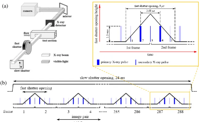
Figure 3.4. (a) Diagram showing light path of X-ray imaging system at the APS (from Khlifa et al. 2017). (b) Synchronization of the shutters, the X-ray pulses and the camera frames to acquire image pairs for PIV analysis.

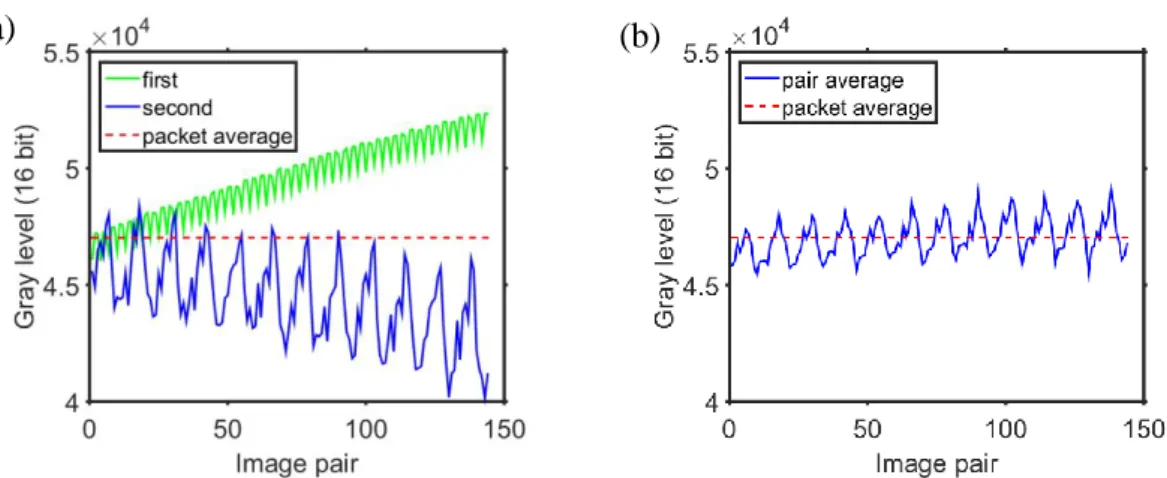
In the beamline, the slow shutter, operating at a frequency of 1 Hz with an opening time of 24 ms, is equipped to protect the test section and the detector by reducing heat load on them. The fast shutter used is a mechanical rotating chopper which operates at a frequency of 6035 Hz with an opening time of 9 μs (Gembicky et al. 2005). Figure 3.4(b) shows the synchronization scheme of the X-ray flashes, the two shutters, and the camera frames, to obtain appropriate pairs of images for PIV analysis. The camera frame transfer is triggered by the secondary pulse 3, so that each image in the same pair could obtain nearly identical illumination. The acquisition frequency of the camera is set to 12 070 fps (twice the fast shutter operating frequency), whichenables a spatial resolution of 704×688 pixels with a pixel size of 2 μm. It should be noted that only a packet of 144 image pairs is recorded during the opening period of the slow shutter (24 ms per second).

(a) 1st frame 2nd frame fa st s h u tt er o p en in g h ei g h t (b)

(33)

22

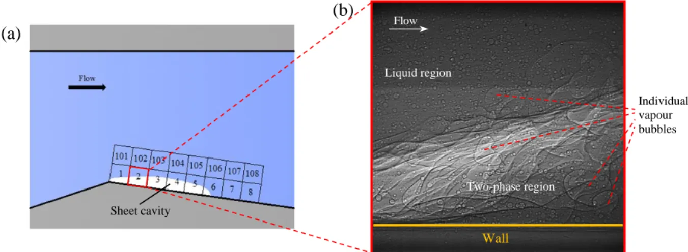
Figure 3.5. (a) Schematic of X-ray beam scanning positions; position 1 corresponds to the beginning of the cavity. The test section was moved to different positions enabling X-ray beam to scan the complete flow field of interest. (b) A representative raw X-ray image of cavitation recorded at the scanning window 2.

Silver-coated hollow glass spheres with nominal mean diameters of 10 and 17µm were injected into the flow as tracers of the liquid phase. Because of the small cross section of the X-ray beam, successive but not simultaneous acquisitions at different positions are necessary to obtain the complete image for the flow field of interest as shown in Figure 3.5(a). To that end, the test section was moved parallel to the divergent floor of Venturi in front of the X-ray beamline by a motorized platform. At each position, 1872 pairs of images are recorded, which are actually divided equally into 13 packets (corresponding to the slow shutter opening 13 times), and thus the time between packets is not continuous.

Figure 3.5(b) presents a typical raw X-ray image of cavitation recorded at the second position. The bright band at the center results from extra partial exposure to a secondary X-ray pulse as indicated in Figure 3.4(b). In addition to absorption contrast, the X-ray phase contrast leads to a fringe pattern with sharp intensity variation along the phase interface, which allows a better visualization of the two-phase flow morphology and the seeded particles. As can be found in the raw radiograph, the vapour structures in the position close to the cavity leading edge are generally coherent except a few individual vapour bubbles identified. The seeded particles both inside and outside the cavity are also visualized clearly. They are much smaller and have relatively regular round shape, compared to individual vapour bubbles.

(a) (b) Sheet cavity Wall Flow Individual vapour bubbles Liquid region Two-phase region

(34)

23 3.4. Data extraction based on image processing

Although the two-phase information is contained simultaneously in the X-ray images, the transition from visualization to quantitative measurement (e.g. velocity and void fraction fields) is not easy. In the conventional PIV images, a high signal-to-noise ratio (hence a distinct cross correlation peak) is achieved by large contrast in gray levels between particles and liquid background as the liquid can rarely scatter laser light. However, due to the relatively bright background associated with X-ray imaging mechanisms, the signal-to-noise ratio would drop greatly if the background is not removed from the X-ray image. In order to analyze the dynamics of each phase, image processing is required to extract the tracer particles from the liquid background and vapour structures so that velocimetry algorithms can be applied to each phase separately.

3.4.1. Separation of the two phases

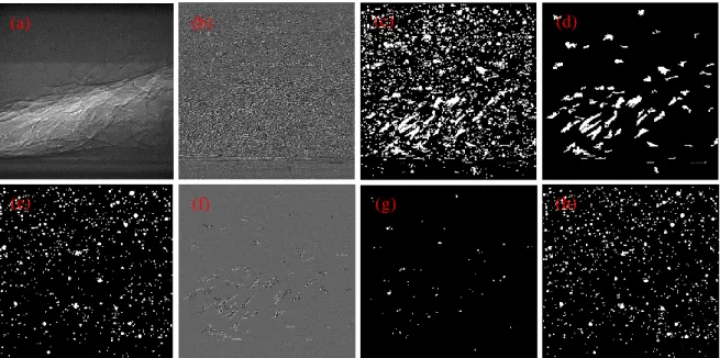
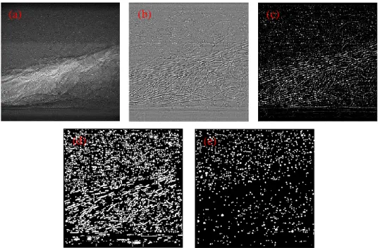
The first attempt to separate the seeding particles and the vapour bubbles could be found in Khlifa et al. (2017) where the liquid background was eliminated based on the vapour volume fraction measurements and large areas of vapour structures were removed using a high-pass filter. This image processing method was greatly dependent on the accuracy of void fraction while the error could be ±15% according to their description if measurements of void fraction were performed using each individual image without pair averaging. In the present work, we employed a new wavelet-decomposition-based image processing method to separate the seeding particles from the non-uniform background of the liquid and the vapour structures. For a smooth narrative, the detailed description of procedures of this new method is provided in Section 3.6. The final result is presented in Figure 3.6. The particle image (Figure 3.6(b)) extracted from the raw X-ray image (Figure 3.6(a)) will be used for the measurements of liquid phase velocities. Figure 3.6(c) shows the remaining vapour structures which will be used for calculating the instantaneous velocity field of vapour phase. It should be pointed out that compared to the first attempt the same raw X-ray images were also used in the present study, nevertheless this new method is not dependent on the void fraction accuracy and is much less time-consuming (approximately 1/3 processing time with the same computing resources).

(35)

24

Figure 3.6. Result of image processing for separation of two phases. (a) Raw X-ray image of cavitation; (b) particle image for measurements of liquid phase velocities; (c) vapour structure image for measurements of gaseous phase velocities.

3.4.2. Void fraction measurement

The local void fraction 𝛼 is defined as the ratio of the vapour volume to the total volume along any given beam path crossing the test section. The value represents the averaged void fraction in the spanwise direction. Since the vapour has a different X-ray attenuation coefficient from the liquid, the local vapour volume fraction 𝛼 could be estimated quantitatively using Equation 3.2, derived from Lambert–Beer’s law,

𝛼 = 1 − ln (_𝐼𝐼0

𝛼) ln (𝐼_𝐼0

1)

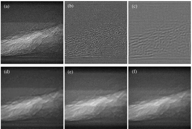
where I0 is the local intensity measured when the test section is completely filled with vapor (for convenience, vapour is replaced here with air as they almost have an identical absorption coefficient), I1 is the local intensity measured when the test section is full of water, and 𝐼_𝛼 is the local intensity measured when cavitation occurs in the test section. For computing 𝛼, it is thus necessary to take the calibration images of air and water under the same acquisition conditions as the cavitation tests. Figure 3.7(a) and (b) show the calibration images for gaseous phase and liquid phase, respectively. They were obtained by averaging a large number of reference images corresponding to each phase. Figure 3.7(c) presents a processed image for the computation of void fraction. The aim of processing the raw image is to reduce the effect of imperfect synchronization and fringes due to X-ray phase contrast mechanism on void fraction measurements. The detailed processing procedures are provided in Section 3.7. The final result of instantaneous vapour volume fraction field is illustrated in Figure 3.7(d).

(a) (b) (c)

(36)

25

Figure 3.7. Measurements of vapour volume fractions, (a) calibration image of air; (b) calibration image of water; (c) processed image for computation of void fraction; (d) vapour volume fraction field.

3.4.3. Particle image velocimetry

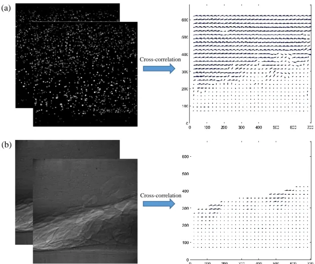
Based on the MatPIV.1.6.1 open source toolbox, cross-correlation algorithm was applied on each pair of consecutive particle images obtained by the aforementioned image processing procedures to determine the corresponding liquid phase displacements. The time delay between the two pictures was 3.68 μs. Four interrogation passes with window offset were carried out and the interrogation window size was progressively decreased in order to increase the spatial resolution.

In the first pass the interrogation window size was set to comply with the one quarter rule to limit in-plane loss of particle pairs. For instance, in the present case where the largest displacement estimated from the flow rate is 20 pixels, a window dimension of 80×70 pixels was chosen with a larger size in the streamwise direction. It should be noted that the correlation coefficient is computed directly in the spatial domain rather than using an FFT-based approach.

(a) _(b)

(37)

26

In spite of its low efficiency, this direct computation allows to eliminate the constraint of equal window size with the power of 2 (32×32 pixels, 64×64 pixels, etc.) required by FFT implementation, and it can be useful to reduce the velocity gradient effect in the direction perpendicular to the flow.

Figure 3.8. Instantaneous velocity vector field evaluated from an image pair, (a) liquid phase; (b) vapour phase.

In the next pass, the refined interrogation windows were shifted locally according to the integer displacement field evaluated from the first pass such that the proportion of matched particle pairs is increased. The final interrogation window size should be made sufficiently small to reduce velocity differences within the interrogation area, meanwhile it is also limited by the particle concentration. To ensure a good signal-to-noise ratio, at least 4 matched particle pairs are required in the last interrogation window. Thanks to the method we use to extract particles from vapour structures, it is easy to know the mean number of particles

(a)

(b)

Cross-correlation

(38)

27

(approximately 1200) in an X-ray image. Therefore, the minimum window size is estimated to be 40×40 pixels. Considering that the particle distribution is not strictly homogeneous, the last window size was enlarged slightly in the main flow direction into 50×40 pixels. This final window size determines the actual spatial resolution in the PIV data which implies that the turbulent structures with scales smaller than this size cannot be resolved.

In the studied cavitating flows, the local velocity field exhibits a strong shear even within the smallest interrogation window. It would make the signal-to-noise ratio decrease drastically and cause a large uncertainty in velocity measurements. In order to solve this problem in regions with high velocity gradient, an image deformation scheme (Raffel et al. 2007) was utilized in the last pass. The correlation peak was estimated with a sub-pixel accuracy by using the three-point Gaussian fitting scheme in two directions.

Figure 3.8(a) shows an instantaneous velocity vector field of the liquid phase evaluated through the above cross-correlation algorithm, in which the aberrant vectors detected by median test were rejected and then replaced by bilinear interpolation from their valid neighboring vectors. The two ends where illumination is not sufficient were excluded. Each pair of processed particle images produced 26×31 local velocity vectors spaced equally by 22 pixels (44 μm).

The same cross-correlation algorithms used for the liquid phase were also applied to each pair of vapour images. Since there are no seeding particles to trace the vapour phase, the cross-correlation is based on the variations of gray levels related to the presence of vapour bubble interfaces and the void ratio difference. Thanks to the calculated vapour volume fraction field, the liquid region was masked out. In practice the measurements of vapour velocities were activated only when the spatially-averaged void fraction within the final interrogation window is greater than 7%. Figure 3.8(b) presents the computed velocity field of the vapour phase.

The uncertainty of the velocity measurements for both phases were discussed in Khlifa et al. (2017). The cross-correlation accuracy of tracer particles was estimated by generating synthetic images of a cavitating flow with imposed particle displacements. The comparison between imposed and measured values shows that the mean error of the liquid phase velocity measurements is around ± 0.24 m/s (approximately 3% of the reference velocity of the studied flow). The uncertainty in vapour phase velocity measurements was also estimated by imposing known displacements on vapour structures of a cavitating flow. The results indicated an error of around ±0.46 m/s (approximately 5% of the reference velocity) for the vapour phase.

(39)

28

3.5. Comparison between conventional laser PIV and X-ray PIV

Unlike the standard PIV measurements where only the particles in a given plane are illuminated with a thin laser sheet, all particles and bubbles along the beam path are projected into the X-ray image due to the line-of-sight nature associated with the X-ray imaging method. Therefore, the standard PIV result represents the 2D velocity field in the illuminated plane while the X-ray PIV result is the span-averaged velocity field containing amassed flow information in the spanwise direction. Lee & Kim (2003) reports the velocity profile in an opaque circular pipe measured by the X-ray PIV method, where the measured velocity at the pipe center is only two-thirds of the theoretical value. This discrepancy is attributed to the three-dimensionality of the laminar flow boundary layer given a mean velocity of 0.5 mm/s in an opaque Teflon tube with an inner diameter of 750 μm.

4 8 12 16 0 1 2 3 Laser PIV X-ray PIV 04 8 12 16 1 2 3 Laser PIV X-ray PIV

Figure 3.9. Comparison of mean streamwise velocity (𝑢) profiles at two locations measured by the standard PIV and the X-ray PIV in the non-cavitating condition, (a) x=8 mm; (b) x=14 mm.

The standard PIV measurements under the non-cavitating condition was also carried out in the Venturi-type test section in order to examine the two-dimensionality of the flow. The central plane of the Venturi channel was illuminated by a thin laser sheet of 1 mm thickness, thus allowing 2D velocity measurements less affected by the two side walls. As shown in Figure 3.9, the mean streamwise velocity profiles measured by the standard PIV and the X-ray PIV are compared quantitatively with each other at two different distances from the Venturi throat (x=8 mm and x=14 mm). Note that the x-axis is along the Venturi divergent floor and the origin is located at the apex of the Venturi throat (indicated in the inset of Figure 3.9). As

𝑢 (m/s) 𝑢 (m/s) 𝑦 (m m ) 𝑦 (m m ) x = 8 mm x = 14 mm (b) (a) Flow