HAL Id: hal-02587704
https://hal.archives-ouvertes.fr/hal-02587704v2
Submitted on 4 Jun 2020HAL is a multi-disciplinary open access
archive for the deposit and dissemination of sci-entific research documents, whether they are pub-lished or not. The documents may come from teaching and research institutions in France or abroad, or from public or private research centers.
L’archive ouverte pluridisciplinaire HAL, est destinée au dépôt et à la diffusion de documents scientifiques de niveau recherche, publiés ou non, émanant des établissements d’enseignement et de recherche français ou étrangers, des laboratoires publics ou privés.
Experimental and Numerical Investigation of the
Fluid-Structure Interaction on a Flexible Composite
Hydrofoil under Viscous Flows
Laetitia Pernod, Antoine Ducoin, Herve Le Sourne, Jacques-André Astolfi,
Pascal Casari
To cite this version:
Laetitia Pernod, Antoine Ducoin, Herve Le Sourne, Jacques-André Astolfi, Pascal Casari. Ex-perimental and Numerical Investigation of the Fluid-Structure Interaction on a Flexible Com-posite Hydrofoil under Viscous Flows. Ocean Engineering, Elsevier, 2019, 194, pp.106647. �10.1016/j.oceaneng.2019.106647�. �hal-02587704v2�
Ocean Engineering, 2019 1 Ocean Engineering, 2019, Editor version: https://doi.org/10.1016/j.oceaneng.2019.106647
Experimental and Numerical Investigation of the Fluid-Structure
Interaction on a Flexible Composite Hydrofoil under Viscous Flows
Laetitia Pernoda,b,*, Antoine Ducoina, Hervé Le Sournec, Jacques-André Astolfid, Pascal Casarie
1
a. Laboratoire d’Hydrodynamique, d’Energétique et d’Environnement Atmosphérique (LHEEA), CNRS UMR 6598, Ecole Centrale de Nantes, Nantes, France
b. Naval Group, Technocampus Océan, Bouguenais, France
10 2
c. Institut de recherche en Génie civil et Mécanique (GeM), CNRS UMR 6183, ICAM Ouest - site de Nantes, Carquefou, France
d. Institut de Recherche de l’Ecole Navale (IRENav), EA 3634, Ecole Navale, 29 240 Brest, France e. Institut de Génie des Matériaux (GeM), CNRS UMR 6183, IUT de Saint-Nazaire, Saint-Nazaire, France * Corresponding author: [email protected], 135 Rue du Faubourg de Roubaix, Parc du Château Blanc, 59 800 Lille
ABSTRACT
This research investigates the fluid-structure interaction and hydroelastic response of a composite hydrofoil using an innovative joint experimental and numerical method. The main novelties are, first, the use of a state-of-the-art strain measurement technique, via a fully-distributed-optical fiber sensor directly embedded within the composite
20
plies. This method allows for a finer representation of the structural deformations under hydrodynamic loading. Second, a tightly-coupled high-fidelity fluid-structure interaction numerical model taking into account the turbulent effects in the flow and the ply-by-ply modelling of the composite, is compared to the experimental results. A composite profile is specifically designed as a trapezoidal hydrofoil and is tested for moderate Reynolds number and pre-stall and post-stall incidences. High-speed imaging of the hydrofoil tip and vibrometer measurements are carried out to determine the experimental tip displacements and hydrofoil’s vibrations. The numerical and experimental results show a very strong hydroeleastic response, with a structural resonance even for low Reynolds numbers due to the high flexibility of the structure. Strong coupling of the fluid and the structure, with lock-in of the von Kármán vortex-shedding to the structure for small incidences, and an excitation of the structure by leading-edge vortex-shedding for higher incidences, are also observed.
30
Keywords
Composite hydrofoil; Fluid-Structure Interaction; tight CFD-FEM coupling; optical fiber sensors; flow-induced vibrations
NOMENCLATURE
V Flow velocity field u Structure displacement field n External normal to the structure fv Volumic forces acting on the structure 𝐷𝐷� Deformation field in the fluid
𝐼𝐼̿ Identity tensor
𝜎𝜎� Stress field
𝜀𝜀̿ Deformation field in the structure
𝜏𝜏�𝑓𝑓 Reynolds stress tensor
Eij Elastic modulus
Gij Shear modulus
Ocean Engineering, 2019 2 ρs Solid density
ρf Fluid density
µ Dynamic viscosity of the fluid
P Pressure field in the fluid
P0 Atmospheric pressure
U0 Incident flow velocity
CL Lift coefficient
CD Drag coefficient
CM Moment coefficient
cmean Hydrofoil mean chord
e Hydrofoil trailing edge thickness
L Span of the hydrofoil
α Angle of attack
α0 Zero-lift angle induced by the hydrofoil
camber
θ Hydrofoil twist angle
δLE Leading edge tip displacement of the hydrofoil
δTE Trailing edge tip displacement of the hydrofoil
Re Reynolds number
fvk Vortex shedding frequency due to von Kármán
h Height of the tunnel squared-test section
y+ Dimensionless wall distance
St Strouhal number
LIST OF ABBREVIATIONS 40
CFD Computational Fluid Dynamics CFL Courant-Friedrichs-Lewy CPU Central Processing Unit CSD Computational Solid Dynamics CSE Co-Simulation Engine DES Detached Eddy Simulation DIC Digital-Image Correlation DNS Direct Numerical Simulation FE Finite Elements
FIV Flow-Induced Vibrations FSI Fluid-Structure Interaction
IRENav Institut de Recherche de l’Ecole Navale LE Leading Edge
LES Large Eddy Simulation LSB Laminar Separation Bubble MAB Manganese-Aluminium-Bronze
MNET Mixed Numerical Experimental Technique NAB Nickel-Aluminium-Bronze
RTM Resin Transfer Moulding TE Trailing Edge
URANS Unsteady-Reynolds-Averaged-Navier-Stokes 1 INTRODUCTION
Marine propellers have been traditionally made from metallic alloys, such as Nickel-Aluminium-Bronze (NAB) and Manganese-Aluminium-Bronze (MAB), which greatly simplify the design and analysis process, as they can
Ocean Engineering, 2019 3
be modelled under the assumption that they are effectively rigid, allowing the hydrodynamic and structural analysis to be decoupled (Phillips et al., 2017). Moreover, the material response of such metallic alloys can be confined to the linear elastic regime, and the associated material failure mechanisms are well quantified (Young et al., 2018). However, metallic alloys now approach their performance limits, as they suffer from poor acoustic damping that can lead to noise, poor electro-magnetic signature, low fuel-efficiency, and are subject to corrosion
50
and cavitation damage, as well as fatigue-induced cracking (Mouritz et al., 2001).
In the last decades, a considerable amount of research has been completed on the potential benefits of composite materials as new technologies to further improve the performances of marine propellers. Indeed, composite materials offer great advantages such as higher strength-to-weight ratios leading to a better fuel-efficiency, improved vibration damping properties, reduced magnetic/electric signatures, higher fatigue life, improved flexibility and potentially lower costs of ownership compared to propellers made from traditional metallic alloys (Motley et al., 2009; Young, 2008). Furthermore, due to their anisotropic properties and improved flexibility, composite materials may exhibit bend-twist and extension-twist coupling behaviours that enable them to passively change shape and adjust to the incoming flow. This passive morphing capability of composite materials is now commonly used in aerospace industry and for wind engineering applications (Murray et al., 2015), and is
60
progressively introduced in maritime applications. Several studies showed that marine composite propellers can be tailored to (i) deliver improved hydrodynamic performances and lower fuel consumption compared to their rigid counterparts in off-design operating conditions and in spatially and/or temporally varying flows (Lee and Lin, 2004; Motley et al., 2009; Young, 2008), (ii) delay cavitation inception (Lee et al., 2015; Motley and Young, 2011; Mouritz et al., 2001) and (iii) reduce the levels of noise and vibrations (He et al., 2012).
Nonetheless, designers of marine composite propellers have to overcome new challenges, as the density of water is three orders of magnitude higher than air, the kinematic viscosity of water is an order of magnitude lower than air, and composite materials are lighter than their metallic counterparts. Consequently, composite propellers are much more prone to fluid-structure interaction (FSI) and development of unwanted hydrodynamic instabilities, such as flow-induced vibrations (FIV) (Young et al., 2018). This makes composite propellers more difficult to
70
model since it is no longer possible to decouple hydrodynamic and structural analyses. As a consequence, it is of primary importance to understand the load-dependent fluid-structure interactions of lightweight flexible composite structures, to characterize the hydroelastic response of such structures, and to identify the influence of the structural properties of composite materials on the hydroelastic response (ply orientation and ply layup). Several methods have been proposed in the literature to study marine composite propellers and composite hydrofoils, both experimental and numerical.
In particular, a number of numerical fluid-structure coupled methods have been developed, namely the
loosely-coupled method and the tightly-loosely-coupled method. The fluid and the structure are modelled as a loosely-coupled system in
which the two media mutually influence each other: the structural motion of the propeller causes a change in the hydrodynamic forces acting on the wetted surface of the structure, which in turn results in a change in the motion
80
of the structure. In the loosely-coupled approach, only one data transfer is realized between the solvers for each time step; on the contrary, the tightly-coupled approach involves several data transfer, referred as coupled
iterations, between the solvers within each time step. The advantages of each class of method have been widely
discussed in the literature, and several improvements to the loosely-coupled approach were proposed (Farhat and Lesoinne, 2000; Felippa and Park, 1980; Kassiotis, 2009; Piperno et al., 1995). Nonetheless, the tightly-coupled method is still recommended for the study of flexible lightweight marine composite structures, as the loosely-coupled methods suffer from a lack of convergence when important added mass is involved. The fluid numerical methods that have been employed for the numerical analysis of the fluid-structure interaction of marine composite structures include inviscid potential flow methods, such as the momentum or blade element method, lifting line method, lifting surface method, panel method and, more recently, viscous flow methods (Computational Fluid
90
Dynamics, CFD). A review of these different fluid methods and their utilisation in the field of numerical fluid-structure interaction is available in the article of Young et al, (Young et al., 2016). Among the viscous flow methods, URANS (Unsteady-Reynolds-Averaged-Navier-Stokes) methods are the most commonly used, as the prohibitive computation times of LES (Large-Eddy-Simulation), DES (Detached-Eddy-Simulation) and DNS (Direct Numerical Simulation) methods make them suitable only for low Reynolds numbers. Moreover, even though URANS methods yields better hydrodynamic performance prediction and more accurate modelling of the turbulent flow surrounding a marine propeller, the computational efficiency of panel methods makes them highly
Ocean Engineering, 2019 4
competitive, and they are thus still widely in use, with new improvements (Li et al., 2018, 2017). Concerning the structure numerical methods employed for the study of FSI on marine composite structures, Finite Element (FE) modelling involving both conventional solid elements for modelling of the homogenized structure, and
100
conventional (thin) shell elements and continuum (thick) shell elements for a ply-by-ply modelling have been used. Indeed, as discussed in (Maljaars et al., 2017), the actual fiber orientation and distribution are difficult to accurately model, but the use of a ply-by-ply modelling allows the subsequent optimization of the composite layup. Optimization schemes considering both the geometry and ply layup of the propeller could indeed also be used in the design loop of these novel marine propellers ((Young et al., 2016) and references therein). Moreover, structural resistance of the composite, cavitation and potential hydrodynamic instabilities can still be assessed with these methods using classical staggered procedures between the solvers. However, (Ducoin et al., 2012b) and (Zarruk et al., 2014) underline the lack of experimental data on the fluid-structure interaction and hydroelastic response of marine composite propellers available in the literature, which leads to few experimental validation of the numerical coupling methods proposed in the research mentioned above.
110
Due to the difficulties of conducting underwater experiments, most experiments were carried out at model scale on simplified geometries of hydrofoils, both under subcavitating and cavitating flows. In 1998, Gowing et al. (Gowing et al., 1998) were among the first to experimentally study composite marine hydrofoils under cavitating flows, and they observed delayed cavitation inception and tip deloading. In 2006, Chen et al. (Chen et al., 2006) studied a small-scale composite propeller and observed improved hydrodynamic performances and cavitation inception. Several subsequent experimental researches were carried out on rigid and flexible hydrofoils vibrations under hydrodynamic loading, such as flow-induced vibrations (Akcabay et al., 2014) and laminar to turbulent boundary layer transition induced vibrations (Ducoin et al., 2012b, 2012a). The influence of hydrofoil trailing edge shapes and structural properties on the vibrations characteristics of the hydrofoils were also investigated (Phillips et al., 2017; Zobeiri, 2012). Experimental investigations were also carried out on the steady-state fluid-structure
120
interaction of flexible composite hydrofoils (Young et al., 2018; Zarruk et al., 2014). (Banks et al., 2015; Marimon Giovannetti et al., 2017) developed an experimental technique using Digital-Image Correlation (DIC) to measure foil deflections under fluid loads. Last, Hoerner et al. (Hoerner et al., 2018) studied the fluid-structure interaction of a flexible composite hydrofoil in forced rotational oscillation motion.
The purpose of this work is to provide some insights into the fluid-structure interaction, hydroelastic response and flow-induced vibrations of flexible composite propellers, thanks to a combined experimental and numerical investigation of a new composite hydrofoil. The numerical approach is based on an implicit Block Gauss-Seidel coupling between a commercial Computational Fluid Dynamics (CFD) solver, Starccm+, and a commercial Computational Solid Dynamics (CSD) solver, Abaqus, that simulates the dynamic behaviour of cantilevered, trapezoidal flexible hydrofoils. Finally, the results are discussed, where hydrofoil deformations, tip displacement
130
and vibrations are analysed by both simulation and measurements.
2 MATHEMATICAL MODEL 2.1 Fluid Governing Equations
In this study the flow is assumed to be Newtonian, incompressible and is modelled using the Unsteady-Reynolds-Averaged-Navier-Stokes (URANS) equations of mass conservation (1) and momentum conservation (2), where ρf is the density, μ is the fluid dynamic viscosity, P the pressure field, V the velocity field, 𝐼𝐼̿ the identity tensor, 𝐷𝐷� the deformations tensor and 𝜏𝜏� is the Reynolds stress tensor. 𝑓𝑓
140
∇ ∙ 𝑽𝑽 = 0 (1)
𝜕𝜕
𝜕𝜕𝜕𝜕 (𝜌𝜌𝑓𝑓𝑽𝑽) + ∇ ∙ �𝜌𝜌𝑓𝑓𝑽𝑽⨂𝑽𝑽� = − ∇ ∙ �𝑃𝑃𝐼𝐼̿� + ∇ ∙ �𝜇𝜇𝐷𝐷� + 𝜏𝜏� � 𝑓𝑓 (2)
Ocean Engineering, 2019 5
The structure is fully submerged and subjected to volumic forces fv. It is characterized by its elastic modulus Eij,
shear modulus Gij, Poisson's coefficients νij and density ρs. Here the variables i and j represent the directions 1 to
3 relative to the ply orientation-angle ϕ, as defined on Figure 1a. The solid problem is solved for the displacements field u via the stress and deformation fields (respectively noted 𝜎𝜎� and 𝜀𝜀̿), and answers to the three following equations: its state law of elasticity expressed by the relation (3), usually known as Hooke's Law, the displacements-deformations relation written for small perturbations (4) and the fundamental law of physics (5).
150 𝜀𝜀̿ = 𝐶𝐶𝜎𝜎� (3) 𝜀𝜀̿ = 12 (∇�𝒖𝒖 + ∇�T𝒖𝒖) (4) ∇𝜎𝜎� + 𝜌𝜌𝑠𝑠𝒇𝒇𝑣𝑣= 𝜌𝜌𝑠𝑠𝜕𝜕𝒖𝒖 2 𝜕𝜕𝜕𝜕2 (5) 2.3 Coupled Equations
The two physics are coupled with a kinematic condition (6) and a dynamic condition (7) written at the interface. The first equation enforces the continuity of velocities at the interface Γ, while the second one is relative to the balance of forces the two media mutually apply one on the other. Note that the vector n represents the external normal to the structure.
∂𝒖𝒖 𝜕𝜕𝜕𝜕 = 𝑽𝑽
(6) 𝜎𝜎� ∙ 𝒏𝒏 = − ∇ ∙ �𝑝𝑝𝐼𝐼̿� + ∇ ∙ �𝜇𝜇𝐷𝐷� + 𝜏𝜏� � 𝑓𝑓 (7)
160
3 EXPERIMENTAL SETUP AND TECHNIQUES 3.1 Experimental Setup and Sensors
3.1.1 Experimental Facility
Experiments were carried out in the hydrodynamic tunnel at the Institut de Recherche de l’Ecole Navale (IRENav) of the French Naval Academy, Brest, France. The tunnel test section is 1 m long with a 192 mm square section for a volume of 60 m3. Available operational velocities in the test section range from 0 m/s to 12 m/s and are set up
using a regulation system Elvovert XD 37kW 400V connected to a pump and an electrical motor. The pump has a
170
precision of 0.1% on the rotational velocity, leading to uncertainties on the free-stream velocity of ΔU0 = ±0.02 m/s. The pressure within the test section can also be set up to specific values between 100 mbars to 3 bars to control cavitation inception, using a regulation system Yokogawa® with a precision of 2.5 mbars. The pressure is monitored using two piezoelectric resistive transducers Paroscientific®: The first one averages the pressure over three pressure sensors (Keller AG 2 MI PAA100-075-010) located upstream of the test section inlet while the second one is connected to one pressure sensor downstream of the test section inlet. Moreover, the effective velocity within the test section is induced from the pressure difference upstream and downstream of the inlet. Finally, a honeycomb grid upstream of the test section allows for a 2% free stream turbulent intensity at the mid-section. For more information about the hydrodynamic tunnel, please refer to (Leroux et al., 2005).
180
3.1.2 Test Setup
The hydrofoil is mounted horizontally in the tunnel test section, clamped at its root and free at its tip. The clamping system allowed variations of the angle of incidence of the hydrofoil, using a step-by-step DC motor with a
Ocean Engineering, 2019 6 precision of ±1/60º. In comparison with the test section dimensions, the hydrofoil dimensions are 90 mm for the mean chord (cmean) and 180 mm for the span (L). Hence the aspect ratio is relatively low (aspect ratio of 2) and the confinement parameter h/cmean=2.13 (where h is the height of the squared-test section) is high enough to consider the confinement effect as small on the hydrodynamic performances. Moreover, since a 1.2 cm gap exists between the hydrofoil and the wall, a tip vortex occurs at the tip of the hydrofoil. Even though these 3D effects are not negligible, the focus of the experiment is to measure the natural frequencies, vibrations and strains experienced by the structure, as well as the tip displacements. Hence it is considered to be an acceptable trade-off to observe
190
increased FSI coupling effects compared to a smaller structure. The velocities considered in this study ranged between 1 m/s and 6 m/s, corresponding to moderate mean-chord Reynolds numbers from 90,000 to 540,000, and the pressure was set at subcavitating flows. A range of angles of attacks from -10deg to +10deg have been tested.
3.1.3 Sensors
The vertical velocities of the vibrations of the hydrofoil are measured using a Doppler laser vibrometer located above the hydrofoil. The laser vibrometer is a PSV-400 developed by Polytec, equipped with a He-Ne laser of visible beam 633 nm (visible infra-red light) whose power is inferior to 1 mW (Class 2 laser). It provides velocity measurements either on a grid of points of up to 512 x 512 points, or at a specific point of the structure. It can
200
measure up to frequencies of 40 kHz and velocities of 10 m/s. High-speed imaging of the tip displacements is realised using a Fastcam SA3 120K (developed by Photron) high-speed camera with an accuracy of ±0.1 mm. The camera is setup with a sampling frequency of 1000 images/seconds and a resolution of 1024 x 512. Additional details relative to the mounting of the hydrofoil in the test section and the measurements methods may be found in (Lelong et al., 2017). Finally, the strains are measured using a distributed-optical fiber directly embedded within the composite plies (additional details are given in paragraph 3.3). The interrogator is a LUNA Rayleigh ODISI-B, provided by LUNA, operating at a frequency of 1 Hz over a 1.23 m length fiber. The fiber provides strain measurements up to ±10,000 micro-strain with an accuracy of ±25 micro-strain at 1,900 points over its length. Figure 1 shows the experimental test setup featuring the hydrofoil within the tunnel test section as well as the laser vibrometer and the high-speed camera.
210
Figure 1: Experimental test setup
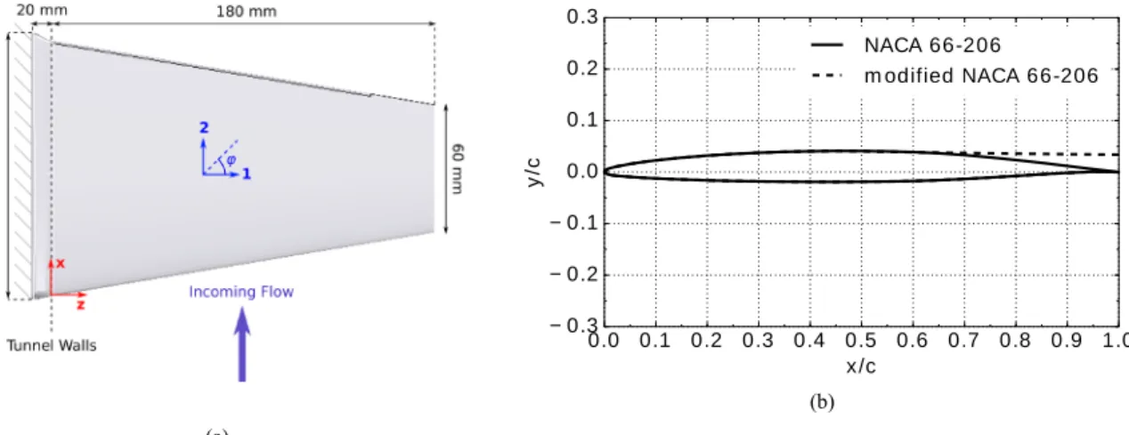
3.2 Hydrofoil Geometry
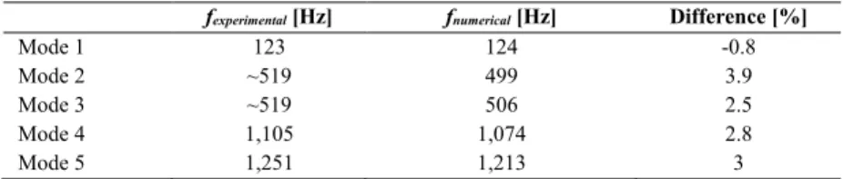
The composite hydrofoil investigated in the present paper is specifically designed to behave similarly to propeller blades operating in a ship wake, when considering both static and dynamic conditions. Based on the work of (Zarruk et al., 2014), the hydrofoil consists of a trapezoidal planform with a base chord of 120 mm and a tip chord of 60 mm for a span of 180 mm, as illustrated on Figure 2a. A cambered NACA 66-206 section is used, which is conventional for propeller blades and well documented at IRENav, where the testing is carried out. The camber is set to 7.6% at 45% of the chord. Moreover, the suction side is thickened to 4 mm at the root and 2 mm at the tip
220
for improved manufacture of the composite materials. The modified section is presented along the initial section on Figure 2b. A thicker section and trailing edge also offer the benefits of potential von Kármán vortex-shedding and flow-induced vibrations (Zobeiri, 2012), of particular interest when investigating fluid-structure interaction
Ocean Engineering, 2019 7
phenomena. The clamping principle is designed to insure the proper sealing of the setup: The 180 mm span is extended by 20 mm at its root (Figure 2a) and inserted within a disk previously imprinted with the shape of the section. This disk is then clamped to a motor in order to vary the incidence of the structure in the hydrodynamic tunnel. Thus, the effective span for the CFD-model corresponds to the wetted surface, that is 180 mm, while the span for the CSD-model is 200 mm in order to account for the added weight and stiffness.
(a)
(b)
Figure 2: (a) Geometry of the hydrofoil viewed from above, (b) Comparison of initial and modified NACA 66-206 sections 3.3 Hydrofoil Materials and Composite Layup
230
The hydrofoil is designed as a sandwich composite structure, that is, a structure made of two thin skins attached on both sides of a lightweight core, as illustrated on Figure 3a. In the present case, the core consists of plies of glass mat fabric made of short unidirectional fibres disposed in such a way that the resulting mat material is quasi-isotropic. Its main function is to help the resin distribution during the manufacture process by RTM (Resin Transfer Moulding Process), thus insuring homogeneous material properties within the structure. Then, two thin skins containing unidirectional glass-epoxy fibers each are stacked on both sides of the mat. The fibres run continuously in the 20 mm extended part of the root. Since the thickness is not constant along the span, some plies need to be progressively reduced and dropped relative to the initial stacking sequence. This is done similarly to the layers of an onion: the central mat fabric is kept along the span, as well as the outer surface ply (to keep a constant surface
240
quality), and the internal plies the closest to the centre are dropped. With this method, four zones containing each a different number of plies are defined on the hydrofoil along the span: the first zone (the closest to the root of the hydrofoil) contains four unidirectional glass-epoxy fibers on each side of the mat, while the fourth zone (the closest to the tip of the hydrofoil) contains only one unidirectional glass-epoxy fiber on each side of the mat. Figure 3b shows the four different zones viewed from above, and Table 1 gives the layup details of each of the zone. Note that the number of plies within the mat material is adjusted to complement the thickness of the geometry. Within this stacking sequence, the plies are laid-up in the following: the outer ply is oriented at 0º (that is along the 1-direction defined on Figure 2a) to insure structural integrityof the hydrofoilwhen subjected to bending, while all the internal plies are oriented at -45º on the pressure side, and at +45º on the suction side. The ply-orientation is defined by the ϕ angle relatively to the 1 and 2 directions on Figure 2a (in the particular configuration shown on
250
Figure 2a ϕ = +45º). The orientation at ±45º is indeed in favour of greater overall flexibility of the structure. Moreover, the non-symmetrical arrangement between the pressure and suction sides leads to an extension-twist coupling effect that opposes the twist of the hydrofoil induced by the incoming flow. As a consequence, the extension-twist coupling effect induces a “de-twisting” of the hydrofoil, which has a stabilizing effect on the flow.
Ocean Engineering, 2019 8
(a)
(b)
Figure 3: (a) Schematic of a composite sandwich section, (b) Plies layup in the hydrofoil featuring the reduction in number of plies along the span, due to the varying thickness
Table 1: Details of the composite plies’ layup
Material Ply orientation Ply thickness Zone 1 Zone 2 Zone 3 Zone 4
UD glass-epoxy fiber 0º 0.15 mm UD glass-epoxy fiber -45º 0.15 mm UD glass-epoxy fiber -45º 0.15 mm UD glass-epoxy fiber -45º 0.15 mm MAT 0º complement UD glass-epoxy fiber 45º 0.15 mm UD glass-epoxy fiber 45º 0.15 mm UD glass-epoxy fiber 45º 0.15 mm UD glass-epoxy fiber 0º 0.15 mm
A very specific and innovator characteristic of the present layup is the direct integration of a fully-distributed-optical fiber within the composite plies. Indeed, a fully-distributed sensing fiber of 1.23 m providing strain measurements at 1,900 points is weaved in the first and second plies of the hydrofoil, in order to measure the deformations for the bending modes (segment [AB] featured in red on Figure 4) and the torsion modes (segments
260
[CD] and [EF] featured in red on Figure 4). This state-of-the-art technique consists of weaving the optical fiber
inside the raw glass-epoxy fibers before their treatment through RTM. This method offers the following benefits compared to traditional strain sensors (e.g. strain gauges and extensometers), as well as traditional use of the optical fiber (i.e. directly tipped to the surface):
• It is possible to define over a thousand sensing areas per meter of fiber, and to weave or curb the said fiber along a path or grid in the structure, which is much more convenient than installing several hundreds of strain gauges
• In the case of fully-distributed sensing fibers, it is possible to dynamically adjust the position of the sensing areas in a couple of minutes, allowing several grids to be tested, while it would take hours to
270
reposition the conventional sensors (in the present study, only one such grid is considered)
• Embedding the optical fiber directly within the composite plies avoids creating local roughness on the structure, which can cause added turbulence and in some cases flow detachment if the roughness size is in the order of the boundary layer thickness
• The use of embedded fiber allows the detection of plies delamination. This aspect is however not considered in the present study.
Ocean Engineering, 2019 9
Figure 4: Direct integration of a 1.23 m fully-distributed optical fiber within the composite plies 3.4 Material and Structural Properties of the Hydrofoil
3.4.1 Material Properties of the Hydrofoil
280
The material and structural properties of the constituents of the hydrofoil are summed up in Table 2. A mixed-numerical-experimental technique (MNET) is first used to check the material properties to use as inputs to the structure solver. Indeed, correct input numerical material properties are a key factor for the accurate Finite Element (FE) modelling of composites; however, their determination most of the time involves destructive measurements. In their recent paper, Maljaars et al in 2017 (Maljaars et al., 2017) tackle this issue of destructive measurements thanks to the introduction of an MNET based on static experiments and a deterministic approach to determine the stiffness properties of small scale composite propeller blades. They also show that the average sensitivities of the in-planes stiffness properties for contact analyses are larger than for the eigenfrequency analyses, advocating the use of static data in the MNET to determine the input numerical material properties.Based on the work of (Maljaars
290
et al., 2017), the composite hydrofoil is tested in air in a cantilevered configuration. The profile is clamped to a table thanks to the vice identified as (2) on Figure 5a, and a 3D-printed part identified as (3) on Figure 5a is mounted on the tip of the hydrofoil. This 3D-printed part is used to load the hydrofoil with masses of 1 kg and 2 kg, as shown for example on Figure 5b. Full-field 3D measurements of the vertical displacement are obtained using two digital stereo-mounted camera and a Vic-3D product for Digital Image Correlation. Figure 6 shows a very good agreement between the experimental measurements (solid lines) and the numerical results (point data) for loads of (a) 1 kg and (b) 2 kg, with a maximum experimental/numerical difference on the vertical displacement less than 6%.
Ocean Engineering, 2019 10
(a)
(b)
Figure 5: (a) Top view of the experimental setup used to check the material properties of the hydrofoil , (b) Front view of the experimental setup with a load of 1 kg.
300
Table 2: Material properties of the hydrofoil
Unidirectional glass-epoxy Mat
Weight [g/m2] 170 100 Density [kg/m3] 1,779 1,578 Volume of fibres [%] 45 30 Ply thickness [mm] 0.148 0.131 E11 [MPa] 34,122 10,783 E22 [MPa] 7,370 10,783 G12 [MPa] 2,168 4,029 G13 [MPa] 2,168 1,656 G23 [MPa] 2,627 1,656 ν12 [-] 0.295 0.338
Tensile strength along 1 [MPa] 930.2 93.9 Compression strength along 1
[MPa] 585.1 95.6
Tensile strength along 2 [MPa] 36.2 93.9 Compression strength along 2
[MPa] 61.6 95.6
Shear strength along 12 [MPa] 20.9 54.2 Shear strength along 13 [MPa] 20.9 25.5 Shear strength along 23 [MPa] 20.9 25.5
(a) (b)
Figure 6: Comparison of experimental measurements (solid lines) and numerical results (point data) on the vertical displacement field for (a) a load of 1 kg and (b) a load of 2 kg.
Ocean Engineering, 2019 11
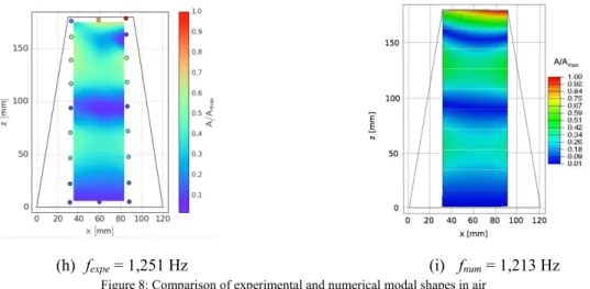
The natural frequencies of the hydrofoil are first determined in air within the empty hydrodynamic tunnel at IRENav. This way the natural frequencies are determined in air and in water under the same clamping conditions. A shaker located below the hydrofoil provides the excitation in air by hitting the hydrofoil at its middle, thus emulating an automated impact hammer. The resulting vibrations of the hydrofoil are measured using a Doppler laser vibrometer located above the profile that maps the surface on a grid of 27 points arranged as a 9 x 3 points. Mapping the complete grid requires 20 min to 30 min.
310
Results of the vibration measurements are presented on Figure 7, with the corresponding mode shapes presented on the left part of Figure 8. The first five natural frequencies are visible: natural frequencies corresponding to modes 1, 4 and 5 are clearly identifiable as, respectively, the first mode of bending, the second mode of torsion and the second mode of bending, while natural frequencies corresponding to modes 2 and 3 are confounded. This is interpreted as the coalescence of modes at the experimental level. Indeed, it is difficult to experimentally discern two modes of very close frequencies, leading the vibrometer to measure at the same time the contribution of modes 2 and 3. Moreover, a numerical modal analysis is performed on the same configuration using the FE commercial code Abaqus/Standard (R.U. Dassault Systèmes, Providence, 2014. Abaqus Documentation - Abaqus Theory Guide), and the numerical natural frequencies in air are compared to the experimental ones in Table 3 (details
320
regarding the numerical models are given in the following sections, in particular section 4.2 for the structural Finite Element model). Mode shapes are compared on Figure 8. Results present a very good agreement, with a difference on the natural frequencies less than 4%, and overall good agreement on the mode shapes, even though some differences are observed close to the tip of the hydrofoil, probably due to the interpolation of the experimental data. It is also very clear from the numerical results that there are indeed two bend-twist coupled modes of close frequency not detected experimentally.
Figure 7: Vibration measurements in air
330
Table 3: Comparison of experimental natural frequencies and numerical natural frequencies in air fexperimental [Hz] fnumerical [Hz] Difference [%]
Mode 1 123 124 -0.8
Mode 2 ~519 499 3.9
Mode 3 ~519 506 2.5
Mode 4 1,105 1,074 2.8
Ocean Engineering, 2019 12
(a) fexpe = 123 Hz (b) fnum = 124 Hz
(c) fexpe = 519 Hz (d) fnum = 499 Hz
(e) fnum = 506 Hz
Ocean Engineering, 2019 13
(h) fexpe = 1,251 Hz (i) fnum = 1,213 Hz
Figure 8: Comparison of experimental and numerical modal shapes in air
The experimental natural frequencies of the hydrofoil are then measured in water at an incidence of 6º, and the excitation is induced by the turbulence from a quasi-steady incoming flow with a Reynolds number of 450,000. In order to reduce the measurement time, the vibrations are measured at a single point. Results of the vibration measurements are presented on Figure 9, where the first nine natural frequencies are visible. Furthermore, the mode shapes in water obtained using a FE code for the first five modes are very similar to the in-air mode shapes (refer again to section 4.2 for details concerning the numerical model). Table 4presents the comparison between the experimental and numerical natural frequencies in water. Comparison of the first five natural frequencies in air and in water shows very significant added mass effects, with a reduction of the in-air natural frequencies
340
between 54.7% up to 66.7%. Indeed, the fluid to solid mass ratio (ρf /ρs) is close to the unity (0.625), meaning that
the inertial effects of the fluid on the structure are dominant.
Figure 9: Vibration measurements at 6º under hydrodynamic flow of Re=450,000
Table 4: Comparison of experimental natural frequencies and numerical natural frequencies in water fexperimental [Hz] fnumerical [Hz] Difference [%]
Mode 1 41 44.6 -8.8 Mode 2 180 200.9 -11.6 Mode 3 220 228.6 -3.9 Mode 4 500 505 -1 Mode 5 540 545.5 -1 4 NUMERICAL METHODS 4.1 Fluid Numerical Model 350
Ocean Engineering, 2019 14
The commercial CFD code Starccm+, based on the Finite Volume method, is used to solve the fluid governing equations introduced in section 2.1. The URANS equations are closed for the Reynolds stress tensor 𝜏𝜏� using the 𝑓𝑓
transport equations from the k-ω-SST turbulence model (Menter et al., 2003). Laminar to turbulent transition could be induced at the hydrofoil surface, as the Reynolds numbers considered are moderate (180,000 < Re < 540,000). As a consequence, the γ - Reθ transition model was used in this study (Menter et al., 2006). The fluid domain and
hydrofoil geometry represent the configuration described in the experimental setup: Figure 10 shows the fluid domain and the mesh used for the simulations, representing the hydrofoil in the tunnel test section with the number of chords upstream of the structure, in the wake and downstream of the structure. An inlet velocity boundary condition is defined at the entrance of the domain, with a steady uniform flow U0 perpendicular to the tunnel
cross-360
section. A turbulent intensity of 2% and a turbulent length scale of 6x10⁻⁴ m are also set at the inlet, which are the
parameters recommended to reproduce the experimental conditions. A pressure outlet boundary condition is set-up at the exit, stating that the pressure field at the boundary matches the atmospheric pressure. The walls of the tunnel are considered as symmetry planes, thus considering the confinement effects without side wall boundary layer modeling. Indeed, because the boundary layer developing on the walls of the test section during the experiments is unknown, it is considered best not to model it. A no-slip condition is enforced at the hydrofoil’s surface for non-coupled simulations and the displacement computed by Abaqus is prescribed for coupled calculations, leading to an imposed velocity boundary condition that satisfies equation (6).
Figure 10: Mesh and fluid domain used in the CFD computations (figure not scaled)
370
The domain is meshed using an unstructured polyhedral mesh with refinement at the leading and trailing edges. The wake is also refined tangent to the trailing edge for about half a chord to accurately capture the von Kármán wake flow. Furthermore, a structured prismatic mesh is used in the vicinity of the wall (at the hydrofoil) to accurately capture the boundary layer developing around the profile. A low y+ approach (y+ < 1) involving a full
resolution of the boundary layer is used, and the transition model γ - Reθ is activated to predict laminar to turbulent
transition. We used this approach in order to accurately predict the boundary layer regimes as well as the wall friction. As a consequence, the associated detachments around the hydrofoil were predicted, and we could capture the unsteady performances mainly seen at low angles of attack (due to von Kármán Wake) and at high angles of attack (due to stall), see section 5.2. An appropriate mesh size was selected thanks to a convergence study on the number of elements in stationary flow, first on the hydrodynamic coefficients, then on the wake of the hydrofoil.
380
Indeed, mesh convergence is reached for 800,000 cells when considering only the hydrodynamic coefficients (see Figure 11), while 6,000,000 cells are required to converge the wake (see Figure 12). As a consequence, a mesh grid of 6,000,000 cells was used for the calculations to be confident that the 3D turbulent effects are well represented.
Ocean Engineering, 2019 15
Figure 11: Mesh convergence on the hydrodynamic coefficients
(a)
(b)
Figure 12: Wake of the hydrofoil for (a) 800,000 cells and (b) 6,000,000 cells.
Unsteady simulations are performed using a second-order backward Euler scheme, with a time step satisfying the condition CFL=U0∆t /∆x < 1. Furthermore, convergence studies are performed on the time step to select the best 390
trade-off between physical accuracy and computation time. It will be shown in the results section 5.2 that the hydrofoil undergoes three different flow regimes with the angle of attacks. Moreover, the physics associated with each of those flow regimes are governed by different time scales. As a consequence, different time steps will be required in the numerical model to reach proper convergence for the different flow regimes. Thus, a convergence study is carried out on angles of attack representative of each of the flow regimes: 0º (unsteady regime due to von Kármán vortex-shedding), 4º (quasi-steady regime) and 9.6º (unsteady regime with nonlinear pre-stall effects and leading-edge vortex shedding). Results are presented on Figure 13. At 0º (Figure 13a), temporal resolutions of 10 -3s and 5x10⁻⁴s are too coarse to accurately discretize the harmonic fluctuations of the lift coefficient, leading to a
triangular representation of the signal. A finer time step of 2x10⁻⁴s captures the correct sinusoidal shape of the
temporal signal, but still presents a significant difference on the amplitude of the signal (16%) as well as a
400
frequency shift relative to the solution obtained for a time step of 10-4s (0.8%), meaning convergence is not reached.
The amplitude difference and frequency shift are respectively reduced to 2% and 0.6% between time steps of 10 -4s and 5x10⁻⁵s; however, computation time increases greatly. Consequently, a time step of 10-4s is used at 0º.
Similar considerations on Figure 13b and Figure 13c lead to respective time steps of 5x10⁻⁴s for 0º < α < 9.6º and
2x10⁻⁴s for α > 9.6º. Indeed, Figure 13c shows that both the amplitude and period of oscillations are not converged
for the configuration dt = 5x10⁻⁴s, contrary to the configuration dt = 2x10⁻⁴s (the amplitude and period are a lot
less different between dt = 2x10⁻⁴s and dt = 1x10⁻⁵s than between dt = 5x10⁻⁴s and dt = 2x10⁻⁴s). Moreover, a time
Ocean Engineering, 2019 16
a proper shape, contrary to the configuration dt = 2x10⁻⁴s. Finally, the difference in results and improved accuracy
between time steps of dt = 2x10⁻⁴s and dt = 1x10⁻⁴s is not much, but the computation time increases greatly. As a 410
consequence, the best trade-off between computation time and accuracy is considered to be dt = 2x10⁻⁴s.
(a) α = 0º (b) α = 4º
(c) α = 9.6º
Figure 13: Convergence study on the time step for (a) α = 0º, (b) α = 4º and (c) α = 9.6º
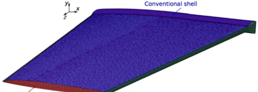
4.2 Structure Numerical Model
The hydrofoil is modeled using the FE commercial code Abaqus/Standard. As stated in the presentation of the experimental setup, the effective span of the hydrofoil for the structure model includes both the wetted surface and the extended root needed to clamp the structure in the water tunnel to account for the added mass and stiffness of this extra material. The methodology used in this study to model the hydrofoil meets the two following objectives: i) accurate ply-by-ply modelling of the composite structure and ii) accurate modelling of the geometric interface
420
between the fluid and solid mediums. Indeed, ply-by-ply modelling of a composite structure makes it easier to study the influence of different ply properties, such as the thickness and the orientation of the plies within the stacking sequence and allows the investigation of different ply configurations for future work. Moreover, coupled computations are carried out via field transfers between the two mediums involved. Therefore, it is of prime importance to accurately model the geometric interface for a correct interpolation of the fields between the solvers. The first objective is usually achieved using conventional shell elements; however, they are surface elements representing only the mid-plane of the composite structure, and consequently do not accurately model the geometric interface. The trade-off used in this study consists of modeling the whole geometry with continuum shell elements (i.e volumic elements associated to shell kinematic properties) filled with mat, and defining a skin of conventional shell elements on both sides of the structure, containing the plies layup (see Figure 14). Using
430
continuum shell elements instead of conventional solid elements is interesting because of their improved representation of strains when the structure is subjected to bending. Moreover, because the thickness is not constant across the composite profiles, the plies are progressively reduced and dropped-off. This particular feature is represented thanks to a division of the hydrofoils in different zones, each with a specific number of plies. Mesh convergence is then realized on the natural frequencies and the maximum tip displacement. For instance, Figure
Ocean Engineering, 2019 17
15 presents mesh convergence on the first two natural frequencies: a total number of 60,141 elements is used for the subsequent computations. Structural computations are first realized under the hypothesis of no geometric nonlinearities, that is small deformations and small displacements. This Finite Element model was used for the modal analysis both in air and in water (the results were presented in section 3.4.2) but with an additional cylindrical acoustic fluid medium surrounding the structure for the modal analysis in water. In this case, the fluid
440
was governed by the Helmholtz equation and sound hard boundaries on all the external faces of the fluid (i.e 𝛁𝛁𝑝𝑝 ∙ 𝒏𝒏 = 0).
Figure 14: Mesh used for the CSD computations
Figure 15: Mesh convergence on the first two natural frequencies of the hydrofoil
4.3 Coupling Algorithm
The coupling is controlled via the Co-Simulation Engine (CSE) developed by Dassault Systems and implemented in Abaqus, and consists of a Block Gauss-Seidel algorithm, that is a tight implicit staggered approach with data transfer at the interface between the fluid and structure solvers. The principle of this algorithm is presented on Figure 16. It consists of iterating over a base cycle within each time step n: (i) The predicted value of the structure
450
displacement field uP,kn+1 is transferred to the fluid solver, (ii) the fluid governing equations are solved for the
pressure pkn+1 and resultant hydrodynamic forces ΦS,kn+1, (iii) the latter are transferred from the fluid to the solid,
so that (iv) the displacement field may now be solved. The use of staggered iterations k between the solvers within one coupling time step helps for the energy conservation at the interface. Moreover, each solver also uses an implicit scheme with internal iterations. To advance in time, the fields transferred must either reach a state of convergence between two coupling exchanges k and k+1 or be forced to move forward after a specified number of iterations Nmax. Here the convergence criterion is set on the displacement thanks to the equation (8).
Ocean Engineering, 2019 18
Figure 16: Tight implicit coupling algorithm 460
4.4 High Performance Computing
The calculations were performed on a BULL/Atos DLC270 cluster at ICI, Centrale Nantes, France. On the one hand, the fluid computations were carried out using the MPI protocol for their parallelization, with an optimal ratio efficiency over number of CPUs around 16 cores Intel Xeon E5v3 (Haswell) distributed on a node Dual x86 at 2.5 GHz. On the other hand, the structure computations were carried out using only one core, due to the licensing options available. However, the latter was not a limiting factor, as the fluid computations and the data transfer between the solvers accounted for more than 64% of the total CPU time. Tightly coupled computations required about 3,400 hours of CPU time to converge, as compared to 15 minutes for the loosely coupled computations.
470
5 RESULTS
5.1 Validation of numerical models against experimental data from the literature (Zarruk et al., 2014)
First, the numerical models are validated against experimental data presented in the literature in (Zarruk et al., 2014) on an aluminum NACA 009 trapezoidal hydrofoil tested in water in a cantilevered configuration. A standalone CFD simulation is first performed, in which the hydrofoil is considered as an infinitely rigid body (i.e. there is no CSD calculation and hence no coupling). Validation of the hydrodynamic coefficients against the experiments is presented on Figure 17, for angles of attack in the range 0º to 14º and an intermediate Reynolds number of 600,000. Results match well when the flow is attached, for 0º < α < 8º, whereas there is an
480
underestimation of lift and of the drag jump after stall occurs. However, those results are classical for URANS computations and may still serve well our purpose of validating the coupling procedure, if we consider an angle of attack before stall. The angle of incidence also needs to be high enough to highlight possible fluid-structure interaction effects, so the loosely coupled and tightly coupled computations are carried out for 6º.
Figure 17: Validation of the hydrodynamic coefficients of lift, drag and moment against experiments from the literature. The accuracy of the absolute position of the indexing system is 0.1º on the angle of attack, and the estimated precision of the force balance on all components is less than 0.5%, (Zarruk et al., 2014)
Loosely coupled computations are then carried out in order to validate the fields transfer between the solvers. It consists of transferring the static pressure field computed during the previous fluid standalone simulation at 6º to the structure solver, and then performing a standalone static finite element simulation on the structure subjected to
Ocean Engineering, 2019 19
this hydrodynamic load (note that the shear stresses are not transferred for loosely coupled computations, but are taken into account for tightly coupled computations). As a consequence, the retroactive loop of the structure on
490
the fluid is not taken into account, and the hydrodynamic coefficients are not updated. Figure 18a shows a comparison of the mesh topology for the fluid and structure models while Figure 18b shows the pressure field computed by the fluid model on the one hand, and the pressure field as transferred and interpolated by a Least Squares scheme to the structure model on the other hand: one can then see that the pressure gradient is correctly interpolated in the CSD code, even though the fluid and structure mesh topologies are quite different.
(a) (b)
Figure 18: (a) Mesh configurations for the fluid and structure models and (b) Validation of the pressure transfer from the fluid solver to the structure solver, suction side
The tip displacements obtained at the leading and trailing edges, and the resulting twist obtained for the loosely and tightly coupled computations, are compared against the experimental data from the literature in Table 5. The results present an overall good agreement with the experiments, as well as some coupling effects on the tip
500
displacements, even if relatively small in the present case. This validation study shows that the numerical coupling method may be applied to the composite hydrofoil developed in this work.
Table 5: Hydrodynamics coefficients, tip displacements and resulting twist compared for the experiments, loosely and tightly coupled computations
CL CD CM δTE [mm] δLE [mm] θ [º]
Experiments 0.53 0.023 0.13 2 2 0
Loosely coupled 0.5 0.03 0.13 1.99 1.96 0.029
Tightly coupled 0.5 0.03 0.14 2.03 2 0.029
5.2 Numerical Study of the Flow Around the Hydrofoil
Figure 19 shows the performances of the hydrofoil for a moderate Reynolds number of 450,000 and angles of attack ranging from -10º to 10º. The corresponding time averaged lift CL, drag CD and moment CM coefficients are
510
reported as square markers and lines, while the fluctuations are represented using red error bars. The lift coefficient shows a quasi-steady behavior for angles of attacks from -7.5º up to +7.5º. The numerical lift coefficients are compared with linear potential theory on a flat plate, expressed by the relation CL=2π(α-α0), where α0 is the
zero-lift angle induced by the hydrofoil camber; in our case, α0 =+0.8º as the trailing edge is modified, which slightly
reverses the camber. Even though this configuration is not optimal in terms of hydrodynamic performances, we consider it to be acceptable, as the main focus is on the investigation of fluid structure interaction. The comparison shows a good agreement between the linear potential theory on a flat plate and the lift coefficients for small incidences, and a greater difference between the two as the angle of attack increases. This highlights the rapid development of viscous effects at the hydrofoil’s surface as the angle of attack increases, as well as the development of a tip vortex.
Ocean Engineering, 2019 20
Figure 19: Hydrodynamic performances of the hydrofoil for a Reynolds of 450,000
Furthermore, the temporal fluctuations of the lift coefficients for incidences of (a) 0º, 2º and (b) 8º, 9.6º and 10º are presented on Figure 20. Two distinct unsteady regimes are identified thanks to the analysis of the time evolution of the lift coefficients and the error bars in Figure 19:
• For -2º < α < 2º, the lift presents a small amplitude, high frequency fluctuations (see Figure 20a), which are maximum at 0º, and progressively vanish for higher and lower angles of attacks. These fluctuations are due to von Kármán wake that develop because of the thick trailing edge
• For α < -7.5º and α > 7.5º, the lift coefficient starts to show non-linearities characterized by the inflection
530
of the lift coefficient curve associated to pre-stall. Moreover, the development of leading-edge vortex shedding induces a multiple low frequency signal, with moderate amplitudes fluctuations that increase with the angle of attack, as shown on Figure 20b and are maximum at 10º.
(a) (b)
Figure 20: Temporal fluctuations of the lift coefficients computed for a Reynolds number of 450,000 and incidences of (a) 0º and 2º and (b) 8º, 9.6º and 10º
Examples of the flow patterns predicted using Starccm+ may be observed on Figure 21 which shows the flow streamlines, the friction coefficient at the hydrofoil surface for Re = 450,000 and incidences ranging from 0º to 10º. A zero-friction coefficient (in white and light brown) represents the separation of the flow, while a negative friction (in blue) coefficient is associated with a recirculation of the flow (vortex). At 0º, the flow is quasi-laminar over the hydrofoil’s surface, with a laminar to turbulent transition occurring close to the trailing edge, and fully
540
turbulent von Kármán alleyways. At 2º, the transition starts roughly around the mid-chord, the flow is fully turbulent at the trailing edge and in the von Kármán wake. The flow at 4º is highly transitional over the whole hydrofoil’s surface, with clear alternate laminar and turbulent zones and a transition triggered by two different mechanisms: a natural transition takes place mostly on the hydrofoil surface (light brown to dark brown color on Figure 21c) while a Laminar Separation Bubble (LSB) is present on part of the leading edge (blue zone circled by red dash), because of high adverse pressure gradient. At high angles of attack, leading-edge vortex occurs (light blue zone on Figure 21d, e and f). It is quasi-stable for 8º and 9.6º. One can also clearly see that the tip vortex induces high friction at the hydrofoil’s tip, which in turn reduces the leading-edge vortex. The symmetry condition
Ocean Engineering, 2019 21 550 (a) α = 0º (b) α = 2º (c) α = 4º (d) α = 6º (e) α = 8º (f) α = 9.6º (g) α = 10º
Figure 21: Flow patterns and skin friction coefficient predicted using Starccm+ for a Reynolds number of 450,000 and different incidences from 0º to 10º
5.3 Numerical and Experimental Static Strains
Static strains were measured using the fully-distributed-optical fiber that was embedded within the composite plies during manufacture. Measurements were carried out on three segments of interest (segment [AB] for bending strains ε11 and segments [CD] and [EF] for torsional strains ε12) for different Reynolds numbers and angles of
attack of -4º, -6º and -9º. Strain dependence to the Reynolds number is first investigated for an angle of attack of -4º, then the influence of the angle of attack on the strains is studied for a Reynolds number of 450,000. Finally, a numerical – experimental comparison is performed.
560
5.3.1 Influence of the Reynolds number
Figure 22 presents the experimental strains of the hydrofoil for different Reynolds numbers and an angle of attack of -4º for (a) bending strains along segment [AB], (b) torsional strains along segment [CD] and (c) torsional strains along segment [EF]. Figure 22a shows a quadratic dependence of the amplitude of the bending strains to the Reynolds number. Moreover, as expected, maximum strains are located near the root of the hydrofoil (z/L = 0mm) and then decrease linearly as we move toward the hydrofoil’s tip. Furthermore, the strains exhibit localized jumps or discontinuities corresponding to the ply drop-offs defined in the composite layup to account for the variable thickness along the span, as discussed in 3.3 and illustrated on Figure 3b: at z0 = 40 mm (z/L = 0.22), z1 = 65 mm
(z/L = 0.36) and z2 = 140 mm (z/L = 0.78). Concerning in-plane shear strains, the strains the closest to the
Ocean Engineering, 2019 22
hydrofoil’s root (segment [EF], Figure 22c) are greater than the strains closest to the tip (segment [CD], Figure 22b). These results demonstrate the ability of the present technique to measure the strain field using embedded fully-distributed-optical fiber.
(a) Segment [AB], α = -4º (b) Segment [CD], α = -4º
(c) Segment [EF], α = -4º
Figure 22: Experimental strains for an incidence of -4º and different Reynolds numbers
5.3.2 Influence of the angle of attack
Dependence of the strains to the angle of attack is presented on Figure 23 for a Reynolds number of 450,000. Similar observations can be done concerning the localized jumps at the ply drop-offs and the increase of the strains with the angle of attack, as expected. In addition, Figure 23b and Figure 23c particularly highlight the greater
580
dispersion and poorer quality of the measurements for the incidence of -9º due to the development of a dynamic flow regime where static measurements are no longer adequate (as presented in section 3.1.3, the acquisition frequency of the strain measures is 1 Hz) . Indeed, as discussed in 5.2, leading-edge vortex shedding associated to pre-stall occurs for α < -7.5º.
Ocean Engineering, 2019 23
(c) Segment [EF], Re = 450,000
Figure 23: Experimental bending strains and torsional strains as a function of the angle of attack for a Reynolds number of 450,000
5.3.3 Numerical – experimental comparison
Figure 24: Map of numerical bending strains for an incidence α = -4º and a Reynolds number Re = 450,000
Figure 24 shows a map of numerical bending strains for an incidence of -4º and a Reynolds number of 450,000.
590
The localized discontinuities corresponding to the ply drop-offs are also well captured by the numerical model. Specific comparisons of the experimental measurements with numerical results from the loosely and tightly coupled computations are presented on Figure 25 for the three segments of interest. The results show that the bending leads to more accurate measurements than the torsion, which can be explained because, as the load increases on the hydrofoil, there is larger relative strains in bending as compared to torsion, and the latter is then subjected to higher relative uncertainties. As an example, segment [CD] in Figure 25b has a mean experimental value of about 120 micro-strain for an uncertainty of ±25 micro-strain. On the other hand, the level of vibrations significantly increases on the whole surface of the hydrofoil, which increases the fluctuations in the strain measurements. Nonetheless, numerical results show a good agreement with the experimental measurements in bending, whereas the measurements in torsion will need further investigations in order to characterize the
600
Ocean Engineering, 2019 24
(a) Segment [AB], Re = 450,000 (b) Segment [CD], Re = 450,000
Segment [EF], Re = 450,000
Figure 25: Comparison between experimental and numerical deformations for loosely-coupled and tightly-coupled computations, for an incidence α = -4º and a Reynolds number Re = 450,000
5.4 Numerical and Experimental Static Tip Displacements
Quasi-static tip displacements are measured from high-speed imaging of the hydrofoil tip under different loading conditions (Reynolds numbers and incidences) at the leading (LE) and trailing (TE) edges (see Figure 26). The displacement is time-averaged over 1000 snapshots during ∆T = 1s. Results are presented on Figure 27a: static displacements share a quadratic dependence to the Reynolds number. Moreover, it shows a linear dependence to
610
the incidence, until around 10º, where the effect of pre-stall is observed. The tip displacement continues to increase, which is expected at it is mainly linked to lift, which is still increasing because the leading-edge vortex is quasi-stable (see section 5.2). Figure 27b presents the twist whenever measurable, derived from the leading and trailing edges displacements thanks to relation (9). Due to the flexibility of the composite materials, tip displacements up to 1 cm may be observed, as well as a twist of 0.8º. The former means that for certain flow regimes, the tip displacements is greater than the maximum thickness of the hydrofoil’s tip (3.6 mm): in such cases, the hypothesis of no geometric nonlinearities made for the numerical modelling is no longer valid (α > 5º). This is a limitation of the current numerical model that should be addressed in further work. The twist also shows a linear dependence to the incidence; however, it clearly decreases when pre-stall starts to occur for an angle of attack of 8º (respectively around -5º). This is due to the large development of the leading-edge vortex that shifts the center of pressure
620
towards the mid-chord of the hydrofoil, which decreases the pitching moment and hence the torsion.
𝜃𝜃 = 𝜕𝜕𝑡𝑡𝑡𝑡−1𝛿𝛿𝐿𝐿𝐿𝐿− 𝛿𝛿𝑇𝑇𝐿𝐿
𝑐𝑐𝑡𝑡𝑡𝑡𝑡𝑡
Ocean Engineering, 2019 25
Figure 26: Quasi-static tip displacement at the leading (LE) and trailing (TE) edges
(a) Experimental static tip displacements (b) Experimental twist at the tip of the hydrofoil Figure 27: Experimental (a) tip displacements and (b) twist at the tip of the hydrofoil for different Reynolds numbers and incidences
Figure 28 presents a comparison of the experimental measurements with the numerical results from the loosely-coupled and tightly-loosely-coupled computations on the static tip displacement for a Reynolds number of 450,000. Results for both the leading edge (LE) and trailing edge (TE) are included. We observe a good correlation of the numerical
630
results with the experimental measurements, with both the trends and orders of magnitude of static displacements correctly predicted by the numerical simulations (bearing in mind that for α > 5º the numerical model probably underestimate the tip displacements because of the geometric nonlinearities). It seems that the difference between the loosely-coupled calculations and the experimental measurements increases with the angle of incidence, that is to say when the deformations of the hydrofoil increases, corresponding to a greater extension-twist coupling effect. However, results as they are do not allow for the moment to conclude on the ability of the tightly-coupled computations to better predict the static displacements.
Ocean Engineering, 2019 26
Figure 28: Comparison of experimental and numerical displacements for loosely-coupled and tightly-coupled computations, for a Reynolds number of 450,000
5.5 Experimental Study of the Hydrofoil’s Vibrations 640
Figure 29 and Figure 30 show the structural vibrations under hydrodynamic flows for incidences of 0º and 9º: the amplitude of the vibrations generally increases with the Reynolds number and the incidence, from amplitudes ranging from -140 dB to -40 dB at an incidence of 0º to amplitudes ranging from -120 dB to -10 dB at an incidence of 9º.
Figure 29a shows the vibration spectra at an incidence of 0º. The natural frequencies are clearly observed (f1 to
f6). It also exhibits additional components, organized by groups of frequencies and identified as fvk. Such groups
of frequencies are related to the vortex shedding process associated with von Kármán alleyways at the hydrofoil’s trailing edge, as we may observe their dependence to the Reynolds number. They are shifted towards the low
650
frequencies when decreasing the Reynolds number. This is confirmed by considering the Strouhal numbers associated to these frequencies, defined by the relation (10), where e is the trailing edge thickness and U0 the flow
velocity, yielding Strouhal numbers in the range 0.2 to 0.3, characteristic of vortex shedding processes. Figure 29b shows the Reynolds-Frequency diagram corresponding to the spectra at 0º, where the linear relationship between the shedding frequency fvk and the Reynolds number may also clearly be seen (the black arrow represents the
frequency shift of the shedding frequency and its interaction with the structure natural frequencies with increasing Reynolds number). In addition, the fact that we observe groups of shedding frequencies, and not only one frequency, is explained by the variable thickness of the trailing edge (from 4 mm at the base of the hydrofoil to 2 mm at the hydrofoil tip). The shedding frequencies act as a source of excitation of the structural vibrations as they interact with the different modes of the hydrofoil. At a Reynolds number of 360,000, the von Kármán process
660
amplifies the amplitude of the third mode by 20 dB, and the damping is significantly reduced. At a Reynolds number of 180,000, the von Kármán frequency matches with the second natural frequency, and resonance is observed, with its two peaks amplified by 40 dB and 60 dB respectively. Because of resonance, harmonics are also clearly observed.
(a) Spectra at 0º (b) Reynolds-Frequency diagram at 0º Figure 29: Vibration measurements at 0º
Ocean Engineering, 2019 27 𝑆𝑆𝑡𝑡=𝑓𝑓𝑣𝑣𝑘𝑘𝑈𝑈𝑒𝑒
0
(10)
For incidences of 9º and higher, the hydrofoil undergoes pre-stall, characterized by leading-edge vortex shedding. The associated leading-edge shedding frequencies fvk are rather difficult to identify in the spectrum (see Figure
30a) because they are located in the low frequencies range, and probably induce multiple frequencies, due to the
670
3D trapezoidal shape of the hydrofoil, as seen numerically in section 5.2. Nonetheless, one can observe the clear resonance of the first mode which is excited by the vortex shedding. This resonance is also clearly visible on the Reynolds-Frequency diagram corresponding to the spectra at 9º on Figure 30b (white peak on the left hand side of the figure).
(a) Spectra at 9º (b) Reynolds-Frequency diagram at 9º Figure 30: Vibration measurements at 9º
6 CONCLUSION AND FURTHER WORK
This study realised a joint numerical and experimental investigation of a composite hydrofoil under hydrodynamic flows. The hydrofoil was specifically designed to behave similarly to a propeller blade thanks to a varying chord
680
along the span, as well as to exhibit an extension-twist coupling behaviour that decreases the twist of the hydrofoil when the hydrodynamic loading increases. This is achieved using a sandwich structure made of unidirectional glass-epoxy fibers with an anti-symmetric stacking sequence over the suction side and the pressure side. Moreover, the trailing edge was made thicker to help with the manufacture of the composite plies. Last, the design of the hydrofoil was also innovative since it included fully-distributed optical fibers directly embedded within the composite plies during manufacture, which is a state-of-the-art strain measurement method.
Loosely and tightly-coupled computations were carried out using an HPC procedure between a CFD commercial code (Starccm+) and a CSD commercial code (Abaqus). The tightly-coupled computations were performed thanks to an implicit partitioned approach (Block Gauss-Seidel) between the fluid solver and the structure solver. Furthermore, the computations involved high-fidelity fluid modelling, capable of capturing the 3D viscous effects
690
in the wake, as well as an accurate ply-by-ply modelling of the composite material. The material properties were checked with a non-destructive mixed-numerical-experimental technique. In addition, a complete set of experiments were conducted in a hydrodynamic tunnel for incidences from -10º to 10º and moderate Reynolds numbers ranging from 90,000 to 560,000. Tip vibrations were measured using a Doppler laser vibrometer, and tip displacements were monitored thanks to a high-speed imaging camera. Last, the deformations of the hydrofoil were also measured using the optical fiber.
Results clearly showed the existence of three different flow regimes: (i) an unsteady flow regime at 0º characterized by von Kármán vortex shedding, (ii) a quasi-steady flow regime for moderate angle of incidences (2º < α < 7.5º) and (iii) an unsteady flow regime characterized by a recirculation zone for pre-stall incidences (7.5º < α < 10º) and leading-edge vortex shedding for post-stall incidences (α > 10º). The two unsteady flow regimes both show
700
very strong fluid-structure coupling due to the high flexibility of the hydrofoil. In particular, it is remarkable that a structural resonance may be observed on the first torsional mode, even for low Reynolds numbers. Lock-in with von Kármán alleyways and structural excitation due to leading-edge vortex shedding are also occurring. Concerning the quasi-steady flow regime, the experimental and numerical static deformations both exhibit some jumps corresponding to the ply drop-offs in the composite layup. The experimental and numerical results also