HAL Id: hal-03047359
https://hal.archives-ouvertes.fr/hal-03047359
Submitted on 8 Dec 2020
HAL is a multi-disciplinary open access
archive for the deposit and dissemination of sci-entific research documents, whether they are pub-lished or not. The documents may come from teaching and research institutions in France or abroad, or from public or private research centers.
L’archive ouverte pluridisciplinaire HAL, est destinée au dépôt et à la diffusion de documents scientifiques de niveau recherche, publiés ou non, émanant des établissements d’enseignement et de recherche français ou étrangers, des laboratoires publics ou privés.
regional climate modelling
Shan Li, Laurent Li, Hervé Le Treut
To cite this version:
Shan Li, Laurent Li, Hervé Le Treut. An idealized protocol to assess the nesting procedure in re-gional climate modelling. International Journal of Climatology, Wiley, 2020, �10.1002/joc.6801�. �hal-03047359�
An idealized protocol to assess the nesting procedure in
regional climate modelling
Shan Li*1,3, Laurent Li*1, Hervé Le Treut2
1Laboratoire de Météorologie Dynamique (LMD), Sorbonne Université, CNRS, École Normale Supérieure, École Polytechnique, Paris, France
2Institut Pierre-Simon Laplace, Sorbonne Université, Paris, France 3IMT-Lille, Douai, France
*Correspondence to:
Dr. Laurent Li
LMD, casier 99, Sorbonne Université 4 Place Jussieu
75252 Paris cedex 05, France Email : [email protected] ORCID : 0000-0002-3855-3976 Publons ResearcherID : X-3278-2019
Or
Dr. Shan Li IMT Lille Douai
CERI Energie et Environnement Site Bourseul, Bâtiment Curie
941 Rue Charles Bourseul, 59500 Douai Email : [email protected]
Short title: An idealized protocol to assess the nesting procedure in RCM
Short abstract in plain text: Nesting an RCM (regional climate model) into a GCM (global
climate model) is generally realized through a relaxation applied at boundaries of the RCM. This procedure of using GCM as a driver to nudge RCM may produce climate deteriorations and biases. The present work elaborates an idealized protocol to assess the uncertainty and performance of the nesting procedure for both long-term mean climate (illustrated here for seasonal-mean T2m drifts) and concomitance of synoptic sequences between the RCM and GCM.
Accepted for International Journal of Climatology August 2020
Abstract. Newtonian relaxation applied at boundaries of RCM (regional climate model) is a
widely-used technique for climate downscaling and regional weather forecasting. It allows RCM to be nested into GCM (global climate model) and to follow the evolution of the latter. An idealized framework to mimic this general practice is constructed with the LMDZ (Laboratoire de Météorologie Dynamique, Zoom) modelling platform and used to assess effects of the relaxation procedure. The assessment is on both synoptic variability and long-term mean. LMDZ is a global atmospheric general circulation model that can be configured as a regional model when the outside domain is relaxed to a driver. It thus plays the role of both GCM and RCM. Same physical parameterization and identical dynamical configuration are used to ensure a rigorous comparison between the two models. The experimental set-up that can be referred to as “Master (GCM) versus Slave (RCM)” considers GCM as the reference to assess the behavior of RCM. In terms of mean climate, there are noticeable differences, not only in the border areas, but also within the domain. In terms of synoptic variability, there is a general spatial resemblance and temporal concomitance between the two models. But there is a dependence on variables, seasons, spatiotemporal scales and spatial modes of atmospheric circulation. Winter/Summer has the most/least resemblance between RCM and GCM. A better similarity occurs when atmospheric circulation manifests at large scales. Weak-correlation cases are generally remarked when the dominant circulation of the region is at smaller scales. A further experiment with identical framework but RCM in a higher resolution allows isolating the effect of relaxation from that of mesh refinement.
Keywords. Regional climate model, Nesting procedure, Climate downscaling, Synoptic
1 Introduction
Global Climate Models (GCMs) are the most advanced tools available to study climate variation at global scale. But they generally have a too-coarse spatial resolution (about hundreds of kilometers) to appropriately investigate regional climate. Climate downscaling, either dynamical or statistical, is thus a necessary step for all issues on regional impacts of global climate change. Climate downscaling in the so-called dynamical approach is generally carried out with a physically-based regional climate model (RCM).
RCM plays an essential role in understanding climate variability and climate change at regional and local scales (Laprise et al., 2008; Rummukanien, 2010; Giorgi and Mearns, 1991). Due to the fact that an RCM is formulated, in majority of the cases, over a limited area, one can go to high spatial resolution with limited computing resources. RCM can be driven by various driving models or datasets such as meteorological reanalyzes, GCMs and other RCMs. RCM generally provides improved climate simulations, especially with respect to statistical properties of extremes, such as cyclones, intense precipitation and strong winds (Giorgi and Mearns, 1991). Improvements can also come from regionally specific empirical adjustments of the model parameterizations.
Meanwhile, RCM is far from being a perfect solution for all needs of climate downscaling. RCM brings added-values with respect to GCM or reanalysis, but it can also present drawbacks. Many challenges still require attention and efforts. First of all, RCM is under constraints, with nudging applied at the lateral boundaries, inconsistent behaviors can occur. Nudging is a simple operation that can be realized by adding a “Newtonian relaxation” in the dynamical equations governing the evolution of wind, temperature and humidity, noted as 𝑋.
𝜕𝑋
𝜕𝑡 = 𝑀(𝑋) + 𝑋𝑜−𝑋
𝜏 (1)
where 𝑀(𝑋) represents the physical laws resolved in the dynamical model, 𝑋𝑜 is the target variable for the nudging, and 𝜏 is the relaxation time scale. The Newtonian relaxation added into the prognostic equations of the model is therefore not a physical term, it can introduce concerns of boundary inconsistency in the model (Giorgi and Mearns, 1991; Denis et al. 2002; Omrani et al. 2012, 2013, 2015; Leps et al., 2019), but it remains a simple and efficient way to drive RCM. It allows us to use outputs of GCM of coarse resolution as lateral boundary conditions (LBC) to run high-resolution regional simulations that evolve over time with GCM. A second caveat in using RCM is the lack of interactive exchanges between RCM and its
driving GCM, since the one-way nesting with a unidirectional nudging is the standard methodology to drive RCM through the outputs of GCM.
In order to understand the behaviors of RCM, it is necessary to separate the various influencing factors for the downscaling ability of the nested RCM. They are at least of three different natures: mesh refinement, downscaling methodology and interaction among spatiotemporal scales. The present work is devoted to dealing with the issue of Newtonian relaxation, the core operation of the downscaling methodology. To isolate its effect, and to understand its role in regional climate simulation, it is necessary to design an idealized framework excluding differences in space resolution and in model physics. We can then focus on methodological issues in relation to the relaxation technique.
The paper is organized as follows. In Section 2, we present the experimental design. Assessment methodology is introduced in Section 3. Section 4 evaluates the effect of Newtonian relaxation by comparing RCM against GCM in six subparts. Subsection 4.1 compares the seasonal mean between RCM and GCM. The spatial resemblance of the atmospheric circulation within the domain is shown in Subsection 4.2. EOF analysis and weather regimes analysis are used in Subsection 4.3 to investigate how the duality RCM/GCM behaves in function of different atmospheric modes or circulation regimes. Subsection 4.4 is devoted to investigating the relationship between external forcing from GCM and the reproducibility of GCM’s synoptic variability by RCM. Subsection 4.5 investigates the sensitivity to the relaxation time and to the update frequency of boundary conditions. Subsection 4.6 shows the effect of RCM mesh refinement. And a variant of our nudging technique with progressive nudging strength is presented in Subsection 4.7 before the presentation of Conclusion.
2 Model configuration and Experimental design
The LMDZ4 model (Laboratoire de Météorologie Dynamique, Zoom version 4) (Hourdin et al., 2006; Li, 1999) is the atmospheric component of the coupled model IPSL-CM4 (Marti et al., 2010) developed and explored at the Pierre Simon Laplace Institute (IPSL). Different versions and configurations of the IPSL model were largely used in climate simulations contributing to the IPCC reports (IPCC, 2007, 2013). LMDZ4 can be operated as a GCM and also as an RCM according to its configurations. In this study, although GCM and RCM are identical, their geographical coverage differs: GCM covers the entire globe, while RCM is effective only in the regional domain considered. Our protocol of simulations can be qualified
as “Master versus Slave”, since both GCM and RCM are identical, but they are operated in a different way: GCM is entirely autonomous (Master) but RCM is driven (Slave) at boundaries (rest of the whole globe beyond its effective domain) by outputs from GCM.
RCM in this study is configured in a large domain extending from the Equator to Greenland (latitude: between 2.4°S and 82.4°N) and from the middle of the North Atlantic Ocean to the Caucasus (longitude: between 40.4°W and 42.4°E). This domain covers regions with varied and complex characteristics, such as the North Atlantic Ocean, Europe, the Mediterranean Sea and North Africa. It therefore includes several sub-regions commonly used in CORDEX studies (Europe, Mediterranean, and Africa) (Giorgi et al., 2009). Jones et al., (1995) showed that the domain size of RCM should be large enough to allow the full development of circulations at fine scales but small enough to maintain suitable control from the driving lateral boundary conditions (LBC). The choice of the domain size is still an open question, but beyond the scope of our study. Our domain includes strong internal variabilities which are believed to be stronger in summer than in winter (Lucas-Picher et al., 2008; Caya and Biner, 2004; Giorgi and Bi, 2000).
The protocol “Master versus Slave” used for this study has a certain resemblance to that of “Big brother versus Little brother” (BBE) proposed by Denis et al., (2002), de Elia et al. (2002) and Antic et al. (2004). BBE protocol consists of performing firstly a GCM simulation with a very high resolution, the same as that of RCM. Horizontal resolution of the output is then degraded to that of a normal GCM. Degraded information is ultimately used to drive RCM. Thus, the climate simulated by GCM with enhanced spatial resolution (called “Big Brother”) plays the role of reference to assess the climate simulated by RCM (called “Little Brother”). Difference between “Big Brother” and “Little Brother” obviously reveals the upmost theoretical performance of RCM. This protocol is particularly interesting for cases where there is no reliable high-resolution dataset to evaluate the performance of RCM. The original geographic domain of interest in Denis et al. (2002) is on the east coastal area of North America, and their model used is CRCM (Canadian Regional Climate Model) (Caya and Laprise, 1999). Although their simulations cover only a month (February 1993), they were able to conclude that the one-way nesting as designed in Davies and Turner (1977) for application to RCM did a good job in climate downscaling from large scales to regional scales. The common point of BBE with our “Master versus Slave” protocol is the concept of perfect model which makes it possible to assess the downscaling approach and the operational
procedure by getting rid of physical imperfections of the climate model used. GCM is actually considered as a “perfect model” and served as the reference for RCM.
Our hypothesis in designing “Master versus Slave” simulations is that there are conceptually two factors affecting the climate downscaling: the general driving methodology of RCM by GCM and the mesh refinement in RCM. To eliminate the effect of RCM resolution, our “Master versus Slave” protocol keeps purposely the two models identical and with the same resolution, about 300 km, a regular grid of 3.75° in longitude and 2.5° in latitude. In the vertical, there are also 19 identical levels for the two models. The particular design of our simulation allows us to have a rigorous comparison between RCM and GCM, since they are actually identical in terms of physics and spatial resolution. This configuration will be hereafter noted as “DS-300-to-300”, standing for “downscaling from 300 km to 300 km”. A comparison between the two models reveals purely the impact of Newtonian relaxation procedure used in driving RCM.
To evaluate the effect of RCM grid refinement, we actually performed a second simulation, just as “DS-300-to-300” in our protocol “Master versus Slave”, but RCM (Slave) has a higher spatial mesh size (100 km, against 300 km in the initial configuration). This additional experiment will be noted hereafter as “DS-300-to-100”, standing for “downscaling from a model of 300 km as spatial mesh size to another model of 100 km”. A relevant comparison between the two experiments can reveal the effect of mesh refinement in RCM, the effect of Newtonian relaxation being eliminated. All simulations of the two experiments have a 360-day calendar (30 360-days for every month). To ensure a good statistical significance, they all have a long duration of simulation exceeding 80 years.
The relaxation time scale ( in Eq. 1) represents the nudging strength. In this study, all variables (winds, humidity, temperature) are strongly nudged since is set at 90 minutes. Boundary conditions from GCM are renewed every two hours. These two parameters are tunable options that may impact the performance of RCM. Two more sets of sensitivity simulations are presented in Subsection 4.5 to see how the simulated climate is sensitive to them.
We remind that our RCM actually covers the whole globe and the buffer zone where relaxation is effective is the rest of the globe outside the RCM domain. There is a sharp transition for the relaxation time scale between the inside (τ=∞) and outside (τ=90 minutes) of the RCM effective domain. In fact, our configuration inherited from a two-way nesting
methodology (as in Chen et al., 2011; Junquas et al., 2015) in which the two models (LMDZ-global and LMDZ-regional) need to be spatially complementary from each other. To mimic more closely the general practice of the research community running RCM, we also include a smooth transition zone in a specific simulation presented in Subsection 4.7.
Both GCM and RCM share the same low boundary conditions with climatological sea-surface temperature and sea ice concentration obtained from 1971 to 2000. They also share the same climatological values for greenhouse gases and aerosols over the period 1971 to 2000.
For the sake of completeness, and to preserve the traceability of our work, in Supporting Information, a document (also available at http://www.lmd.jussieu.fr/~li/LMDZ4_compilation.docx) (or in Li et al., 2020) provides detailed information and guidance to compile the code and to run simulations presented in this work. An archived and compressed file (available at http://www.lmd.jussieu.fr/~li/LMDZ4_code.tar.gz, or in Li et al., 2020) contains the computing source code, and a second archived and compressed file (available at http://www.lmd.jussieu.fr/~li/LMDZ4_data.tar.gz, or in Li et al., 2020) provides configuration files, boundary conditions and job-launching shell scripts.
3 Assessment methodology
Numerical climate model simulations are affected by various uncertainties due to internal variability, and sensitivity to initial conditions and to boundary conditions (Giorgi and Mearns, 1991; Murphy et al., 2004). The evaluation of RCM is often based on mean climatological state of relevant variables such as surface air temperature and precipitation. A few studies also check the synoptic variability. One needs even to assess the synoptic sequences if RCM is destined for regional weather forecasting. Intuitively, we can imagine that the reproduction of regional climate depends on two factors, the external forcing from GCM (reproducible component depending on boundary forcing of GCM) and the internal dynamics (non-reproducible) that develops independently in GCM and RCM. Even in a very restrictive framework, the internal dynamics developing within the region can be quite spontaneous (Separovic et al., 2015, 2008, Christensen et al., 2001). Whatever is the climate downscaling protocol, the internal dynamics can occur and makes RCM to drift significantly from GCM. Generally speaking, the internal dynamics can come from a better resolution, an advanced physics and the climate downscaling protocol itself. In the past, the protocol issue has never been properly evaluated, since it could not be easily isolated. This is just the focus of our
current study. Our basic working hypothesis is that large-scale information of regional climate in RCM should be consistent with that of the GCM because the RCM is under the constraints of GCM. At the same time, we recognize that, within the domain, regional climate dynamics can also be generated by internal processes. We thus expect, when GCM exerts a dominant constraint on the regional climate, to obtain a good resemblance between RCM and GCM. On the other hand, when the large-scale circulation is weak and the internal dynamics is strong, RCM is expected to diverge substantially from GCM.
Daily geopotential height at 500 hPa (Z500) and surface air temperature at 2 meters (T2M) are used to assess the reproduction of the large-scale atmospheric circulation. Separovic et al. (2008, 2015) have shown that the relaxation procedure impacts firstly synoptic (intra-seasonal) scale, an essential element of the atmospheric general circulation (Christensen et al. 2001; Separovic et al., 2015, 2008). Furthermore, synoptic (intra-seasonal) variability is a very important window for internal variability of a model to manifest and to operate (Separovic et al., 2008, 2015; Alexandru et al., 2007; Christensen et al., 2001; Jones et al., 1995). These arguments motivate us to focus on synoptic variation scales to describe the resemblance between RCM and GCM, with the objective to reveal effects of Newtonian relaxation in regional climate modelling. In order to isolate the synoptic or intra-seasonal variability, daily outputs of both RCM and GCM are linearly decomposed into four components, namely the mean state, the inter-annual variation, the seasonal cycle, and finally the intra-seasonal or synoptic variation.
To assess the resemblance between RCM and GCM, we perform spatial correlation on daily variables from RCM and GCM for their synoptic variation (including intra-seasonal scale). The distribution of these spatial correlation coefficients is then examined with box-whisker plots to show their statistical properties. Intuitively we can expect that the resemblance between RCM and GCM is dependent on atmospheric general circulation structures at different scales. We thus perform EOF analysis and weather regimes analysis to illustrate this dependence.
4 Results
4.1 Deviation of mean climate
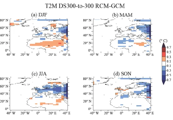
As expected, RCM shows deviation in its mean climate compared to the reference from GCM. Figure 1 displays the difference maps, in the form of seasonal average, of surface air
temperature at 2 meters between RCM and GCM. RCM can reproduce main features of the mean climate simulated by GCM. This is generally true over all the four seasons (DJF, MAM, JJA, and SON). However, there is a significant cooling of more than 1 °C at the eastern border for all seasons. Furthermore, differences are also observed inside the domain. The differences are quite pronounced during DJF and JJA, with a warming of about 0.3 °C in sub-Saharan Africa and over the Atlantic Ocean, and a cooling of about 0.6 °C for the summer (JJA) in Eastern Europe. The fact that RCM deviation is dependent on seasons is certainly a revelation that the basic climate matters for RCM to reproduce the mean climate of GCM. Nevertheless, we should point out that the magnitude of climate deviation in RCM is an acceptable one compared to our general skill in simulating regional climate with the most advanced dynamical modelling tools. Furthermore, we also performed an identical experiment, but with future global warming as the background climate (results not shown here). A very similar deviation was obtained there, showing that the general approach practiced by the regional climate modelling community is a reliable one in terms of future climate projection.
4.2 How close is RCM to GCM in terms of synoptic variability
The protocol “Master versus Slave” provides an idealized (but ideal) framework to evaluate effects of the downscaling procedure. Recall that in this study, RCM and GCM have the same physical and dynamical configurations, apart from the relaxation procedure applied in RCM. In the previous section, the comparison of mean climate between RCM and GCM shows significant differences not only at borders but also within the domain. It is clear that certain autonomy of RCM can manifest in our Master/Slave configuration, even RCM and GCM are identical.
Beyond issues on mean climate, RCM can also show deviations from GCM for day-to-day variations. This is a crucial issue if RCM is destined for weather forecasting or any other operational services (e.g. exploitation of renewal energy), since the synoptic sequence matters. For each day, we can now compare physical fields between RCM and GCM only for their synoptic variability. We investigate how close RCM is to GCM for their simulated synoptic variability. The resemblance between RCM and GCM can be measured by the spatial correlation coefficient of the fields between the two simulations. The physical variables of our investigation are the geopotential height at 500 hPa and surface air temperature at 2 meters. They are examined for the whole year and for the four seasons separately. The surface air temperature at 2 meters is an emblematic climate variable with large implication to societal
issues, and the geopotential height at 500 hPa is an appropriate variable to describe the atmospheric general circulation at middle level.
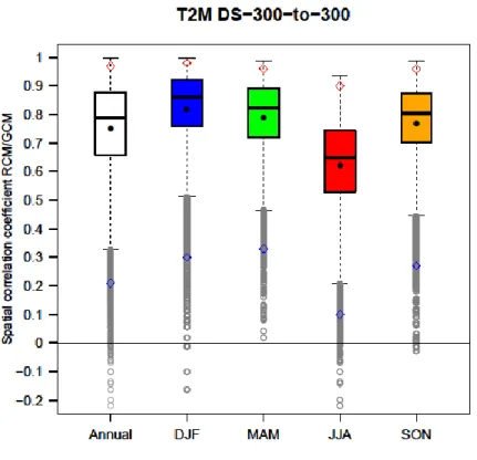
The ensemble of spatial correlation coefficients forms a complex distribution that can be represented in a box plot graph. Results are shown either for the whole year or for the four seasons separately. The averages in the form of a small dot in the box plots are all below the medians (Fig. 2). This relationship between the mean and the median reveals a biased distribution and the presence of a small number of very small values. Weak correlation means big disagreement of spatial structures in the two models. That is, RCM shows its maximum autonomy and losses driving signal from GCM. At the same time, the spatial correlation coefficients have also a tendency toward higher correlation. In fact, a Fisher z-transformation would give approximately a normal distribution for correlation coefficients, since fields from RCM and GCM can be considered as identically distributed and independent.
The box plots for T2M (Fig. 2) and Z500 (Fig. 3) show all an obvious seasonal dependence. A higher spatial correlation with a smaller dispersion (interquartile gap) is found in winter. That is, winter represents a better spatial resemblance between RCM and GCM. Summer shows the lowest spatial resemblance between the two models for both T2M and Z500. The largest correlation coefficient from T2M is 0.98 (maximum) in winter, 0.90 in summer and 0.96 in spring and autumn. The box size (interquartile gap) and the gap of outliers are two parameters to measure the dispersion of spatial correlation coefficients between RCM and GCM. Seasonal characteristics are clearly shown on the box plot. There is a larger dispersion in summer than in winter (Fig. 2).
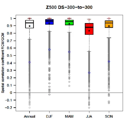
Figure 3 summarizes the statistics of correlation coefficients for the 500 hPa geopotential height. For the whole year and the four seasons, a good correlation is noticed with an average exceeding 0.80 and a median exceeding 0.90. The spatial correlation coefficients for Z500 show the same seasonal variation as for T2M. RCM has the best skill in reproducing the synoptic variability of GCM in winter and the worst in summer. However, the spatial correlation coefficients for Z500 (Fig. 3) are generally higher than for T2M (Fig. 2), with furthermore a smaller dispersion. It is clear that there is a better reproduction at altitudes than near the surface. GCM exerts stronger control at altitudes than at the surface, the RCM autonomy being certainly amplified by surface processes and feedbacks.
4.3 Main modes of regional variability and relationship to RCM skill
The spatial correlation coefficient analysis in the previous section shows there is a better resemblance between RCM and GCM in winter. We have all our intuitive arguments to think that the skill of RCM in reproducing synoptic variability of GCM is dependent on regional circulation modes. Different modes should make RCM to behave differently although the relaxation operation is identically added at the boundaries of RCM without any differentiation of scales or modes. Our study domain is dominated by the North Atlantic Oscillation (NAO), with intermittent appearance of other modes of regional variability. We perform EOF analysis (Fig. 4, 5) and weather regime analysis to identify the main modes dominating the regional variability. Such modes or regimes are then used to stratify the correlation coefficients.
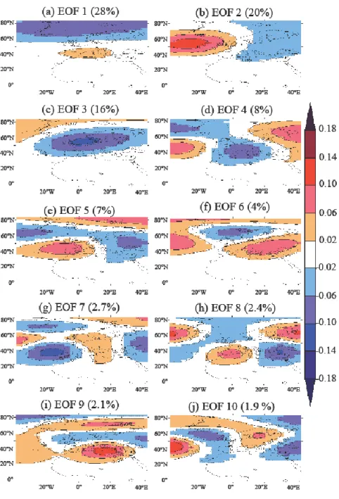
The analysis is again applied to daily data of geopotential height at 500 hPa retaining the only synoptic variability of the atmospheric circulation, after eliminating the mean seasonal cycle. The EOF analysis gives, in descending order of explained variance, the dominant spatio-temporal patterns, and leaves the noise in the EOF structures of higher order. In order to compare the time series (PC: principal component) characterizing the synoptic sequence, it is necessary to have a series of common spatial structures for RCM and GCM. To do so, we just joined the two datasets together to perform the analysis in a combined way. We obtained very close results (not shown) if we perform the analysis to one dataset and project the spatial structures to another. The first ten structures representing a variance contribution over 92% are shown in Fig. 4. The analysis was done separately for the four seasons. Only winter is shown for the sake of conciseness. Winter reveals the strongest resemblance between the two models. Similar results are noticed in other seasons.
The explained variance and spatial structure scale both decrease for higher-order EOFs in Fig. 4. The first three EOFs show large-scale structures, which have a contribution of 65% to the total variance. The first EOF shows essentially a north-south bipolar structure between the Greenland Sea and the Mediterranean Sea. It represents the North Atlantic Oscillation, the most important mode of variability in this region. The second EOF also represents a bipolar structure, but with contrasts between the East (Central Europe) and the West (Middle North Atlantic). The third EOF shows a remarkable oval structure, centered in the North Sea with an extension from the middle of the Atlantic to the Caucasus. At the same time, there is a weak expression with opposite sign towards Greenland and the Red Sea. It seems that this structure is in very weak relation with the outside, because it has practically no loading in border zones. The fourth and fifth EOFs both represent a structure like horse-saddle (Fig. 4). Their
contribution in variance also remains very close, and around 7.5% for both. They represent a structure that propagates: a movement in counterclockwise rotation is visible between these two structures. The sixth EOF is an oval structure stretched from Greenland to the Barents Sea with a center on the Norwegian Sea. This structure is encompassed by opposed values, with a strengthened loading in the middle of the North Atlantic, the Balkan and the Arctic Ocean. Higher order EOFs (from 7 to 10) show smaller scales with a wave number around 2.0.
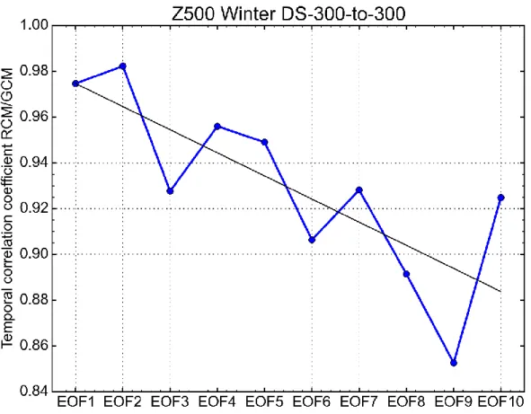
With common spatial structures, it is now useful to compare the corresponding time series between RCM and GCM. Our purpose is to check if some modes promote (or induce) a good (or bad) temporal concomitance between RCM and GCM. Remember that RCM is a constrained model with control from GCM at the outside of its effective domain, through a relaxation operation. It is expected that different structures have their own behaviors in response to constraints from the boundaries. In other words, the influence of external forcing from outside of the domain might be different for different spatial structures. We perform then a correlation calculation between the two corresponding temporal series for each EOF structure to show how their similarity varies for different dominant modes. The reproduction in RCM of the temporal variation of GCM is represented by a correlation coefficient, as shown in Fig. 5. A low temporal correlation coefficient reflects non-concomitant variations of synoptic sequences between the two models. In other words, a low temporal correlation coefficient means that the two models do not vary at the same time in the same mode.
We can see that the two models are generally close to each other for all the shown EOFs, with correlation coefficients all greater than 0.84. A very strong resemblance (correlation coefficient greater than 0.95) is found for the first five EOFs. EOF3 has the lowest correlation coefficient (0.93) among them, but it is still greater than those for smaller scale modes (from EOF6 to EOF10) which have a correlation coefficient around 0.90. For the first two EOFs which contribute nearly half of the total variance to the physical field, RCM and GCM are very close to each other with a correlation coefficient larger than 0.97. The trend line in Figure 5 clearly shows that the concomitance of synoptic sequences between the two models decreases from large scales to small scales. It is clear that the effect of the relaxation operation is dependent on spatial scales. It creates a favorable situation for RCM to behave with greater freedom at small scales than at large scales.
Figures 4 and 5 reveal that the control from GCM to RCM depends not only on spatial scales, but also on spatial modes. Some modes show a weaker concomitance between the two models such as EOF3, EOF6 and EOF9. They all have an oval structure around 60° N (Fig. 4) and
poorly connected to the boundaries. This is especially true for EOF3 in which the isolated oval structure presents a large geographical extension covering Europe and the North Atlantic. The oval structure noticed in these three EOFs makes RCM easier to have larger freedom to manifest its own behaviors, and the temporal evolution between the two models is less concomitant.
It is now clear that the downscaling procedure with the relaxation operation diverts the spatiotemporal variability of RCM from GCM, although their divergence remains weak. Especially, it ensures a good simultaneity between the two models at large scales. RCM shows however more freedom at small spatial scales.
The EOF analysis is a powerful tool in decomposing atmospheric variability. But it remains a mathematical manipulation and the obtained structures can be devoid of any meteorological significance. We need thus to find a complementary way to check the robustness of results. The concept of weather regimes might be a very appropriate one to do so. In mid and high latitudes, quasi-stationary states of atmospheric circulation are recurrent and can be easily recognized at synoptic scale. They are often referred to as weather regimes or circulation regimes (Michelangeli et al., 1995). In the geographic sector Europe / North Atlantic, four weather regimes are generally recognized (Vautard, 1990). They are: NAO+ (zonal), NAO-, blocking and Atlantic Ridge. Different circulation regimes are discriminable for the regional atmospheric circulation and for the regional weather. For example, the zonal regime is linked to winter storms and the blocking regime is associated to cold weather. We can imagine that the resemblance between RCM and GCM may be very dependent on the regional weather regimes. For the sake of conciseness, detailed results are not shown, but as expected, the resemblance between RCM and GCM varies after the stratification of synoptic variability into weather regimes. A low resemblance between the two models is noticed for the blocking regime. This means that RCM has more freedom to not follow GCM under the blocking regime. The dependence of RCM behaviors on regional dominant circulation regimes was also demonstrated in Becker et al. (2015) who used an RCM configured over Western Europe and forced by 6-hourly outputs of a GCM for 41 years. They showed that the cluster with a strong northwesterly flow crossing the full length of the Alpine mountain range provokes the most remarkable RCM-own circulation.
4.4 Dependence of RCM skill on the forcing strength from GCM
Conceptually, the skill of RCM to reproduce the synoptic variability of GCM can be considered as dependent on the driving strength that GCM exerts on RCM, and on the autonomous capacity of both models to develop independent variabilities. The former should enhance the resemblance of models and is reported in this paper; the latter should diminish the skill of RCM and will be reported in future. The intensity of the external forcing is diagnosed by the spatial variance of geopotential height at 500 hPa at the outside of the RCM effective domain. The meridional variance from GCM, at the meridian 45° W close to the effective domain of RCM, can be a good choice for our purpose. Our tests (not shown here) with different locations reveal that results are not very sensitive to the precise geographic positions.
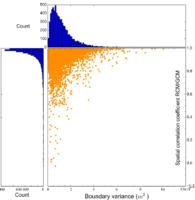
Figure 6 displays the scatter plot (a dot per day, with only synoptic variability) with the spatial correlation coefficients between RCM and GCM for the 500-hPa geopotential height anomalies, plotted from -0.1 to 1.0 in y-axis, in function of the spatial variances of the 500-hPa geopotential height at 45°W in GCM in x-axis (between 0 and 12x104 m2). The scatter plot is completed by two histograms revealing the marginal distributions following the two axes. We can see that the resemblance between the two models increases with the intensification of external forcing. This means that a strong GCM control favors having a good similarity between RCM and GCM. Figure 6 also reveals that low correlation coefficients (less than 0.5) are associated with a very small variance of GCM. However, a weak external forcing does not always imply a bad resemblance between the two models, since the internal dynamics from both GCM and RCM also matters.
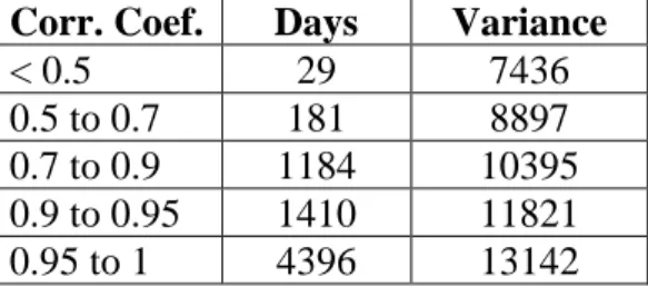
Table 1 presents a numerical summary of what shown in Figure 6. First, we can see that the two models are generally very close to each other with a spatial correlation coefficient greater than 0.95 in 4396 days out of 7200 (61.1%). On the other hand, there are only 29 days out of 7200 (0.4%) with a low resemblance characterized by the correlation coefficient smaller than 0.5. Second, the average of the GCM variance at the boundary of RCM has an obvious relation with the correlation coefficient. When the correlation coefficient is low, the GCM variance at the boundary is also small, and a high correlation corresponds to a high variance.
In summary, the interior of the RCM domain is more or less controlled by large-scale circulation coming from GCM beyond the RCM effective domain. The strong external forcing manifested by a high value of variance at the boundary, favors a good reproduction of
RCM towards GCM. On the other hand, a weak external forcing makes the effect of the internal dynamics more important, which causes a divergence to the two models.
4.5 Sensitivity to relaxation time and to update frequency of boundary conditions
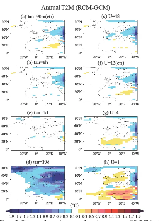
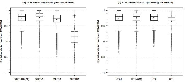
In our experimental protocol, there are two free parameters that may change the behavior of our RCM. The first one is the relaxation time scale τ determining the strength of the nudging. The second parameter is the temporal update frequency (noted as U) of the boundary conditions. Both parameters have implications beyond our framework, since they can raise issues for all RCMs. Due to historical reasons, the two parameters in our control simulation were set at 1.5 hours for τ, and 12 times per day for U (i.e., boundary conditions updated every two hours). In parallel to the control simulation, six other simulations were also performed, under the same conditions, but τ set at 6 hours, 1 day and 10 days, U set at 48, 4 and 1 times per day, respectively. As the control simulation, these six simulations were all run for 80 years. The case of U=48 corresponds to updating boundary conditions every half an hour, the time step for calling physical parameterizations. The case of U=4 is to update boundary conditions every six hours, a common practice for running an RCM with outputs of GCM. We use the same metrics as previously used to evaluate these additional simulations, i.e., deviation maps of RCM from GCM for long-term mean climatology (shown in Fig. 7), and boxplots showing the statistical properties of all spatial correlation coefficients between RCM and GCM for their synoptic variability (shown in Fig. 8).
Let us now examine the sensitivity to variation of τ. In terms of deviation maps, the first three cases are very close to each other. The boundary effect even diminishes from τ=1.5 hours to τ=6 hours, then to τ= 1 day. It is clear that a too-strong nudging deteriorates the consistency at borders. For the agreement of synoptic variability between RCM and GCM, however, the first two cases are very close, but the case of τ= 1 day shows a deterioration. The last case of τ= 10 days shows a very bad situation in both Fig. 7 and Fig. 8. Obviously, a too-weak nudging would loss the control of GCM on RCM. As a whole, we can conclude that the optimal choice of τ would be a few hours. Our control simulation using 1.5 hours for τ seems a case of too-strong nudging with more visible problems at borders.
For the sensitivity simulations with four different values of U (update frequency), the first three cases, with U=48, 12 and 4, show very close results in both Fig. 7 and Fig. 8. The last case of U=1 obviously shows significant deterioration. We can see that updating boundary conditions at interval of a few hours can guarantee a good consistency
between GCM and RCM. The critical point seems situated between 6 hours and 1 day. Our idealized experimental design can thus confirm that the general practice of the regional climate modelling community by putting the update frequency at 4 times per day is a quite reasonable choice. Our results here are consistent with Leps et al. (2019) who used the COSMO-CLM model (COnsortium for SMall scale Modeling, CLimate Mode, German regional climate research community model) under idealized synoptic situations and within the framework of Big-Brother experimental protocol.
4.6 Effect of mesh refinement
In previous sections, all analyzes are based on idealized experiment without a finer mesh size for RCM. The application of mesh refinement at the regional scale is necessary because the coarse mesh of GCM is not sufficient to correctly simulate the regional climate (Giorgi and Mearns, 1991; Jacob et al., 2007; Laprise et al., 2008; Rummukainen, 2010). Furthermore, the horizontal resolution is an important issue for regional climate modelling. Our framework is therefore completed by a second simulation (“DS-300-to-100”) in which the RCM has an increased spatial mesh size (100 km), with all other aspects unchanged. The comparison between the two configurations helps to reveal the impact of mesh refinement in RCM whose effect is added to that of the nesting procedure.
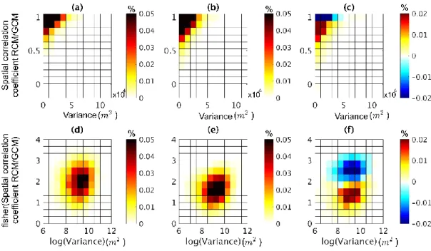
The bi-histograms in Figure 9 show the same relationship between the external forcing and the correlation coefficient characterizing the spatial resemblance of the two models, Fig. 9a being directly deduced from the scatter plot shown in Fig. 6. With mesh refinement (Fig. 9b), a strong external forcing is always associated with a high value of spatial correlation coefficient and a very low correlation value is always in situations of weak external forcing. In both protocols, there are a large number of very strong correlation coefficients with moderate variances (Fig. 9a and 9b). A visual comparison between Figure 9a and Figure 9b shows a shift of the point cloud to the end of low spatial correlation coefficients between RCM and GCM. That means from “DS-300-to-300” to “DS-300-to-100”, there is a trend toward lower consistency and bad resemblance between RCM and GCM. The decrease of correlation (resemblance) following the mesh refinement is obviously noticed on the subtraction of the two protocols (Fig. 9c).
The most significant difference between “DS-300-to-100” and “DS-300-to-300” is found in the range with the external variance less than 20000 m2 and a spatial correlation coefficient exceeding 0.70 (Fig. 9c). Compared to “DS-300-to-300”, “DS-300-to-100” presents a
decrease about 40% (-0.08/0.2, relative changes of probability density function) for high spatial correlation coefficients which exceeds 0.93. At the same time, there is an increase in probability density function for the range of correlation coefficients between 0.70 and 0.93. An obvious increase about 60% (0.03/0.05) is found for the correlation coefficient range between 0.80 and 0.93, and a smaller increase of 30% when the correlation coefficient is between 0.70 and 0.80.
To make the bi-histogram more symmetrical, a Fisher z-transformation, 𝑧 =
1
2ln (1 + 𝑟) (1 − 𝑟)⁄ , is applied for the spatial correlation coefficient and a natural logarithm
is used for the variance. A shift to the left of the center of high probability (Fig. 9d,e) is noticed with a decrease in the upper 50 percentiles and an increase in the lower 50 percentiles (Fig. 9f). The decrease amplitude is larger than the increase. The comparison between “DS-300-to-100” and “DS-300-to-300” clearly shows that the mesh refinement in RCM decreases the spatial resemblance between RCM and GCM.
4.7 Hard versus soft boundaries
The way of introducing boundary conditions into limited-area modelling was always a crucial issue for regional weather/climate simulations. We used in this paper a Newtonian relaxation procedure with a very short time scale (90 minutes). There is no smooth transition zone in our protocol since the relaxation time scale jumps from 90 minutes to infinity within a single model grid. This choice is justified by the fact that our grid mesh size is coarse (around 300 km). Furthermore, our configuration was initially designed for performing two-way nesting between LMDZ-global and LMDZ-regional, which imposes the geographic complementarity on the globe to avoid numerical resonance between the two models. This choice corresponds to what WRF (Weather Research and Forecasting modeling system) does for its two-way nesting configuration (Skamarock et al. 2005, sections 6.4 and 7.3). Our procedure, without a smooth transition zone in the relaxation operation, can be called as a configuration with hard boundaries, in contrast to soft boundaries using a predefined smooth transition zone. In this section we present an additional simulation to show how our models behave similarly or differently between the configuration with hard boundaries and that with soft boundaries.
As explicitly mentioned in Davies (1976) for the first time, it is necessary to use an appropriate way to take into account time-varying boundaries for regional atmospheric modelling. A theoretical consideration was deduced in the framework of a vorticity equation that was used in first-generation numerical weather forecasting models. The work of Davies
(1976) was furthered by other researchers (Robert and Yakimiw, 1984) and also extended to models with shallow-water equation (Davies 1983; Yakimiw and Robert, 1990; Marbaix et al. 2003) and with advection equation (Lhemann 1993). But it seems that such an analytical consideration was never successfully applied to modern regional weather/climate models based on primitive equations, certainly due to their complexity and the presence of nonlinear sub-grid physical processes.
Those models widely used in the regional climate modelling community employs pragmatically a transition zone at their boundaries by varying progressively the nudging strength (Warner et al. 1997). Both WRF (Skamarock et al., 2005, section 6.4) and MM4 (Anthes et al. 1987, section 5.5) use the methodology proposed by Davies and Turner (1977) with a Newtonian term and a diffusion term implemented into the predefined transition zone. RegCM (Regional Climate Model system, Giorgi et al. 1993) uses a very similar approach, but with a larger transition zone and an exponential variation for the nudging strength. Furthermore, it seems that an introduction of water vapor inflow and outflow treatment reduces spurious precipitations at the downstream boundaries. REMO (REgional climate MOdel, Jacob and Podzun, 1997) employs 8 grids as the transition zone. CRCM (Canadian Regional Climate Model, Laprise et al. 1998) uses, at the lateral boundary of the domain, a buffer zone of nine grid-points where model variables are relaxed towards driving data, with a strength varying as a cosine square of the distance from the boundary. When the regional model in UK Met Office is nested into the Unified Model (targeting both weather and climate uses), a transition of 4 grids is used, as described in Jones et al. (1995). Davies (2014) tested an improved nesting scheme in Met Office Unified Model with a blending zone at the boundary of the regional model. It was shown that if the two models have the same space and time resolution, the numerical configuration can keep a precise solution in the blending zone.
To investigate potential differences between the hard boundaries used in this paper and soft boundaries with a sponge zone (a configuration more commonly used in current RCMs as described previously), we transformed our hard-boundary configuration into a soft-boundary one by adding a smooth transition zone at the boundaries of LMDZ-regional with varying nudging strength. The transition zone now covers 4 grid-points with relaxation times of 90, 540, 3240, 19440 minutes respectively (a factor of six, each grid). This new simulation was run for 30 years. A comparison with the same 30 years from DS-300-to-300 (hard-boundary configuration) is presented. Figure 10 displays the surface air temperature changes (RCM minus GCM) for the two configurations. The upper panel is the same as shown in Figure 1,
but for annual mean (instead of seasonal means) and for only 30 years (instead of 80). The lower panel is from the new configuration, showing a much-reduced boundary effect, as expected and in full agreement with what reported in the literature. It is also consistent with our sensitivity experiment, reported in Section 4.5, with longer times for the relaxation time scale τ. Although using a sponge zone reduces boundary effects, there are still significant effects inside the domain, less well organized compared to the hard-boundary configuration.
Let us now examine how the synoptic variability of GCM is reproduced in RCM in terms of surface air temperature. For each day of the 30-year simulations, we can calculate the spatial correlation coefficients and the root-mean square errors for the synoptic variability. Figure 11 displays the statistical properties of these two datasets in the form of box-and-whisker plots. It is easy to see that the soft-boundary configuration diminishes the resemblance between RCM and GCM, since there is a robust decrease of the spatial correlation coefficients (with median value from 0.79 to 0.69, mean value from 0.75 to 0.65) and an increase of the RMS errors (with median value from 0.95 to 1.18°C, mean value from 1.00 to 1.26°C). Such a situation is a little surprising for us, since we intuitively thought that the soft-boundary configuration would increase the control from GCM to RCM. In fact, it reduces only spurious effects near boundaries, but deteriorates the synoptic-scale control of GCM exerting on RCM. By considering the results of sensitivity experiments of τ and U in Section 4.5, we can feel that there is a delicate balance between the control of GCM on RCM and the boundary effect.
It is to be noted that we used here an arbitrary relaxation profile in the transition zone and Marbaix et al. (2003) showed clearly that the transition size and the transition profile can both impact the performance of RCM (MAR in their case). We also note that our soft-boundary configuration enlarged a little the RCM domain, since the transition zone is applied to the external side of the effective domain. This may also contribute to the diminution of control in RCM.
5 Conclusion
This paper was devoted to the investigation of effects of a largely-used climate downscaling procedure which uses a Newtonian relaxation in order to drive RCM with outputs from GCM. We designed an idealized framework, called “Master versus Slave” in which GCM and RCM are identical, but GCM is operated autonomously and RCM is relaxed to GCM at boundaries. The fidelity of RCM to an identical GCM is firstly analyzed (experiment “DS-300-to-300”). The GCM was used as the reference to evaluate the RCM. We thoroughly examined the
spatial-temporal resemblance between RCM and GCM. We also performed the analysis with a stratification of regional atmospheric circulation into different modes or regimes which are believed to play a discriminant role in the relation RCM/GCM. Finally, the intensity of external forcing is also revealed to be a determinant factor for the resemblance between the two models.
In terms of mean climate, RCM can reproduce main spatial patterns of 2-m surface air temperature and 500-hPa geopotential height as in GCM. But significant differences do manifest, especially at borders of RCM effective domain, due to the inevitable conflict between imposed external forcing from GCM and internal dynamics in RCM. Beyond the difference found near the boundaries, we also found significant differences for the whole domain. If the former can be simply treated by an exclusion of the boundaries from analysis, the later may raise issues for climate downscaling.
Beyond the mean climate simulated in RCM, we also examined the synoptic sequences reproduced by RCM and their resemblance to those in GCM. We found that there is a certain dependency on seasons and regional atmospheric circulation modes or regimes. The resemblance between the two models is shown to be stronger in winter than in summer, in larger scales than in smaller ones. Furthermore, the blocking regime in the region seems to have a larger autonomy in RCM. The results are generally in agreement with our expectation, since the reproduction of synoptic sequences is a compromise between the external forcing from GCM and the internal dynamics generated in RCM. The external forcing was thoroughly examined. Strong external forcing promotes a good spatial resemblance and a good temporal reproduction of RCM towards GCM. However, the external forcing does not always guarantee to have a good coherence of regional climate simulation between the two models, because of the impact of relaxation procedure. The relaxation procedure is characterized by the e-folding time scale. It is to be noted that RCM variables under relaxation at borders can never attain the target from the driving GCM, before the target itself is updated when GCM progresses in time. In fact, the initial difference between RCM and GCM diminishes by a factor of 1 − 1 𝑒⁄ (0.63) for each time interval of e-folding time.
This work is a first step to investigate the commonly-used methodology of driving RCM through lateral boundary conditions. We also investigated the impact of GCM updating frequency (every two hours in our work) and that of the relaxation time scale (set to 90 minutes here), which reveals a delicate balance between the need to minimize the spurious border effect and that to keep a tight control of GCM on RCM. Our results confirm that the
6-hourly updating frequency, generally practiced by the regional climate modelling community, is a good choice which does not significantly alter the performance of RCM. For the relaxation time scale, the interval of 90 minutes seems too short, since it enhances the border effect. The choice of a few hours would be recommended for future works.
The internal atmospheric dynamics come from two sources of variability. On the one hand, there is a relation with the continuity of the movement coming from the outside of the domain and the physical-dynamical law governing the continuity of the atmospheric general circulation. On the other hand, regional climate dynamics are also generated by local processes within the study domain, independently of what happens outside the region. The internal dynamics has more freedom in refined RCM which is impacted by more detailed surface process. The mesh refinement increases RCM’s autonomy, with less dependence on GCM. In other words, there is more development of the internal dynamics when the spatial resolution of RCM is increased. Further results on internal variability and its influences on the reproduction of climate and synoptic sequences in RCM will be reported in a future work.
Finally, we believe that our “Master versus Slave” protocol and the main results obtained with this protocol are relevant for other RCMs, although we recognize that our choice of hard boundaries with the platform LMDZ is not the general practice of the regional climate modelling community, due to the absence of a smooth transition zone with progressively variable nudging strength. In fact, the sensitivity experiment specially designed with a smooth transition zone (soft boundaries) shows close behaviors compared to the case of hard boundaries, despite an increase of the deviation between RCM and GCM. This degradation of statistical properties seems due to changes of the domain size and the relaxation time scale, but not related to the relaxation procedure itself. We also want to remind that our RCM used in this work is of very low resolution, compared to more recent practices. A higher-resolution RCM would increase its autonomy and show more deviations from the driving GCM.
Supplementary materials. The online version of this paper contains Supplementary materials
describing how to compile LMDZ and how to run simulations. It is also available with the link http://www.lmd.jussieu.fr/~li/ LMDZ4_compilation.docx.
Code and data availability. The general description of this model can be found at
https://cmc.ipsl.fr/ipsl-climate-models/ipsl-cm4/. The code used in this study is provided with the link http://www.lmd.jussieu.fr/~li/LMDZ4_code.tar.gz (Li et al., 2020). Configuration files, boundary conditions and job-launching scripts are provided with the link http://www.lmd.jussieu.fr/~li/LMDZ4_data.tar.gz (Li et al., 2020).
Competing interests. The authors declare no competing interests
Author contribution. All authors contributed to the design of the experiment and to the
manuscript writing. Shan LI analyzed the simulations and prepared the draft manuscript. Laurent LI developed the model coupling code and performed the simulations.
Acknowledgements. This paper is about a part of Shan Li’s thesis prepared in Sorbonne
Université and LMD (Laboratoire de Météorologie Dynamique) in Paris. Thanks to Sorbonne Université, LMD and Institute Pierre Simon Laplace (IPSL). The Institute for Development and Resources in Intensive Scientific Computing (IDRIS) and the Mesocentre of IPSL provided computing resources for simulations and data processing. Shan Li would also like to thank Patricia Cadule for her comments on the manuscript, for her suggestions, discussions and encouragements during the thesis preparation.
References
Alexandru, A., de Elía, R., and Laprise, R. (2007) Internal variability in regional climate downscaling at the seasonal scale. Monthly Weather Review, September: 3221-3238. doi: https://doi.org/10.1175/MWR3456.1.
Anthes, R. A., Hsie, E. Y., and Kuo, Y. H. (1987) Description of the Penn State/NCAR Mesoscale Model: Version 4 (MM4). NCAR Technical Note NCAR/TN-282+STR, doi:10.5065/D64B2Z90.
Antic, S., Laprise, R., Denis, B., and de Elia, R. (2004) Testing the downscaling ability of a one-way nested regional climate model in regions of complex topography. Clim Dyn 23: 473-493. doi: https://doi.org/10.1007/s00382-004-0438-5.
Becker, N., Ulbrich, U., and Klein R. (2015), Systematic large-scale secondary circulations in a regional climate model. Geophys. Res. Lett., 42, 4142–4149. doi:10.1002/2015GL063955.
Caya, D., and Biner, S. (2004) Internal variability of RCM simulations over an annual cycle. Clim Dyn 22: 33-46. doi: https://doi.org/10.1007/s00382-003-0360-2.
Caya, D., and Laprise, R. (1999) A semi-implicit semi-lagrangian regional climate model: The Canadian RCM. Mon Weather Rev 127: 341-362. doi: https://doi.org/10.1175/1520-0493(1999)127<0341:ASISLR>2.0.CO;2.
Chen, W., Jiang, Z., Li, L., and Yiou, P. (2011) Simulation of regional climate change under the IPCC A2 scenario in southeast China. Climate Dynamics, volume 36, Issue 3-4, pp 491-507. doi: https://doi.org/10.1007/s00382-010-0910-3.
Christensen, O. B., Gaertner, M. A., Prego, J. A., and Polcher, J. (2001) Internal variability of regional climate models. Clim Dyn 17: 875-887. doi: https://doi.org/10.1007/s003820100154.
Davies, H. C. (1976) A lateral boundary formulation for multi-level prediction models. Quart. J. Roy. Meteor. Soc., 102, 405–418.
Davies, H. C. (1983) Limitations of some common lateral boundary schemes used in regional NWP models. Mon. Wea. Rev., 111, 1002–1012.
Davies, H. C., and Turner, R. E. (1977) Updating prediction models by dynamical relaxation: an examination of the technique. Quarterly Journal of the Royal Meteorological Society 103: 225-245. doi: https://doi.org/10.1002/qj.49710343602.
Davies, T. (2014) Lateral boundary conditions for limited area models. Quarterly Journal of the Royal Meteorological Society, 140 (678), 185–196.
de Elía, R., Laprise, R. and Denis, B. (2002) Forecasting skill limits of nested, limited-area models: a perfect-model approach. Monthly Weather Review 130: 2006-2023. https://doi.org/10.1175/1520-0493(2002)130<2006:FSLONL>2.0.CO;2.
Denis, B., Laprise, R., Caya, D., and Côté, J. (2002) Downscaling ability of one-way nested regional climate models: The Big-Brother Experiment. Clim Dyn 18: 627-646. doi: https://doi.org/10.1007/s00382-001-0201-0.
Giorgi, F. and Bi, X. Q. (2000) A study of internal variability of a regional climate model. Journal of Geophysical Research: Atmospheres 105: 29503-29521. doi: https://doi.org/10.1029/2000JD900269.
Giorgi, F. and Mearns, O. (1991) Approaches to the simulation of regional climate change: A review. Review of Geophysics 29: 191-216. doi: https://doi.org/10.1029/90RG02636.
Giorgi, F., Jones, C. and Asrar, G. R. (2009) Addressing climate information needs at the regional level: The CORDEX framework. WMO Bull., 58, 175–183.
Giorgi, F., Marinucci M. R., de Canio G., and Bates, G. T. (1993) Development of a second-generation Regional Climate Model (RegCM2). Part II: Convective processes and assimilation of lateral boundary conditions. Mon. Wea. Rev., 121, 2814–2832.
Hourdin, F., Musat, I., Bony, S., Braconnot, P., Codron, F., Dufresne, J. L., Fairhead, L., Friedlingstein, P., Grandpeix, J. Y., Krinner, G., LeVan, P., Li, Z. X., and Lott, F. (2006) The LMDZ4 general circulation model: climate performance and sensitivity to parametrized physics with emphasis on tropical convection. Clim Dyn 27: 787-813. doi: https://doi.org/10.1007/s00382-006-0158-0.
IPCC (2013) Climate Change: The Physical Science Basis. Contribution of Working Group I to the Fifth Assessment Report of the Intergovernmental Panel on Climate Change [Stocker TF, Qin D, Plattner GK, Tignor M, Allen SK, Boschung J, Nauels A, Xia Y, Bex V and Midgley PM (eds.)]. Cambridge University Press, Cambridge, United Kingdom and New York, NY, USA, 1535 pp.
IPCC (2007) Climate Change: Synthesis Report. Contribution of working Groups I, II and III to the Fourth Assessment Report of the Intergovernmental Panel on Climate Change [Core Writing Team, Pachauri RM and Reisinger A (eds)]. Geneva, Switzerland, 104pp.
Jacob, D., and Podzun R. (1997) Sensitivity studies with the regional climate model REMO. Meteorology and Atmospheric Physics 63: 119– 129.
Jacob, D., Barring, L., Christensen, O. B., Christensen, J. H., de Castro, M., Déqué, M., Giorgi, F., Hagemann, S., Hirschi, M., Jones, R., Kjellstrom, E., Lenderink, G., Rockel, B., Sanchez, E., Schar, C., Seneviratne, S. I., Somot, S., van Ulden, A., and van den Hurk, B. (2007) An inter-comparison of regional climate models for Europe: model performance in present-day climate. Climate Change 81: 31-52. doi: https://doi.org/10.1007/s10584-006-9213-4.
Jones, R. G., Murphy, J. M., and Noguer, M. (1995) Simulation of climate change over Europe using a nested regional-climate model. I: Assessment of control climate, including sensitivity to location of lateral boundaries. Quarterly Journal of the Royal Meteorological Society 121: 1413-1449. doi: https://doi.org/10.1002/qj.49712152610.
Junquas, C., Li, L., Vera, C.S., Le Treut, H., and Takahashi, K. (2015) Influence of South America orography on summertime precipitation in Southeastern South America. Climate Dynamics, volume 46, Issue 11-12, pp 3941-3963. doi: https://doi.org/10.1007/s00382-015-2814-8.
Laprise, R., Caya, D., Giguère, M., Bergeron, G., Côté, H., Blanchet, J.-P., Boer, G. J., and McFarlane, N. (1998) Climate and climate change in western Canada as simulated by the Canadian Regional Climate Model. Atmos.–Ocean, 36, 119–167.
Laprise, R., de Elía, R., Caya, D., Binner, S., Lucas-Picher, P., Diaconescu, E., Leduc, M., Alexandru, A., and Separovic, L. (2008) Challenging some tenets of Regional Climate Modelling. Meteorology and Atmospheric Physics, 100: 3-22. doi : https://doi.org/10.1007/s00703-008-0292-9.
Lehmann, R. (1993) On the choice of relaxation coefficients for Davies lateral boundary scheme for regional weather prediction models. Meteor. Atmos. Phys., 52, 1–14.
Leps, N., Brauch, J., & Ahrens, B. (2019) Sensitivity of limited area atmospheric simulations to lateral boundary conditions in idealized experiments. Journal of Advances in Modeling Earth Systems, 11, 2694–2707. https://doi.org/10.1029/2019MS001625.
Li, S., Li, L. & Le Treut, H. (2020) An idealized protocol to assess the nesting procedure in regional climate modelling. International Journal of Climatology. Zenodo, http://doi.org/10.5281/zenodo.3998323.
Li, Z. X. ( 1999 ) Ensemble Atmospheric GCM Simulation of Climate Interannual Variability from 1979 to 1994. Journal of Climate 12: 986-1001. doi : https://doi.org/10.1175/1520-0442(1999)012%3C0986:EAGSOC%3E2.0.CO;2.
Lucas-Picher, P., Caya, D., Biner, S., and Laprise, R. (2008) Quantification of the lateral boundary forcing of a regional climate model using an aging tracer. Monthly Weather Review 136: 4980-4996. doi : https://doi.org/10.1175/2008MWR2448.1.
Marbaix, P., Gallée, H., Brasseur, O., and van Ypersele, J.-P. (2003) Lateral boundary conditions in regional climate models: A detailed study of the relaxation procedure. Mon. Wea. Rev., 131, 461–479.
Marti, O., Braconnot, P., Dufresne, J.-L., Bellier, J., Benshila, R., Bony, S., Brockmann, P., Cadule, P., Caubel, A., Codron, F., de Noblet, N., Denvil, S., Fairhead, L., Fichefet, T., Foujols, M.-A., Friedlingstein, P., Goosse, H., Grandpeix, J.-Y., Guilyardi, E., Hourdin, F., Idelkadi, A., Kageyama, M., Krinner, G., Lévy, C., Madec, G., Mignot, J., Musat, I., Swingedouw, D., and Talandier, C. (2010) Key features of the IPSL ocean atmosphere model and its sensitivity to atmospheric resolution. Climate Dynamics, Volume 34, Issue 1, pp1-26. doi: https://doi.org/10.1007/s00382-009-0640-6.
Michelangeli, P.-A., Vautard, R., and Legras, B. (1995) Weather Regimes: Recurrence and Quasi Stationarity. Journal of the Atmospheric Sciences Vol. 52, No. 8, pp1237-1256. doi: https://doi.org/10.1175/1520-0469(1995)052<1237:WRRAQS>2.0.CO;2.
Murphy, J., Sexton, D., Barnett, D., Jones, G., Webb, M., Collins, M., and Stainforth, D. (2004) Quantification of modelling uncertainties in a large ensemble of climate change simulations. Nature 430, 768–772. https://doi.org/10.1038/nature02771.
Omrani, H., Drobinski, P., and Dubos, T. (2012) Investigation of indiscriminate nudging and predictability in a nested quasi-geostrophic model. Quarterly Journal of the Royal Meteorological Society 138: 158-169. doi: https://doi.org/10.1002/qj.907.
Omrani, H., Drobinski, P., and Dubos, T. (2013) Optimal nudging strategies in regional climate modelling: investigation in a Big Brother experiment over the European and Mediterranean regions. Clim Dyn 41: 2151-2470. doi : https://doi.org/10.1007/s00382-012-1615-6.
Omrani, H., Drobinski, P., and Dubos, T. ( 2015) Using nudging to improve global-regional dynamic consistency in limited-area climate modeling: What should we nudge? Clim Dyn 44: 1627-1644. doi : https://doi.org/10.1007/s00382-014-2453-5.
Robert, A., and Yakimiw, E. (1986) Identification and elimination of an inflow boundary computational solution in limited area model integrations. Atmos.–Ocean, 24, 369–385.
Rummukainen, M. (2010) State-of-the-art with regional climate models. WIREs Climate Change 1: 82-96. doi: https://doi.org/10.1002/wcc.8.
Skamarock, W. C., Klemp, J. B., Dudhia, J., Gill, D. O., Barker, D. M., Wang, W., and Powers, J. G. (2005) A Description of the Advanced Research WRF Version 2. NCAR Technical Note NCAR/TN-468+STR, doi:10.5065/D6DZ069T.
Separovic, L., Husain, S. Z., and Yu, W. ( 2015 ) Internal variability of fine-scale components of meteorological fields in extended-range limited-area model simulations with atmospheric and surface nudging. Journal of Geophysical Research: Atmospheres, 120: 8621-8641. doi: https://doi.org/10.1002/2015JD023350.
Separovic, L., de Elía, R., and Laprise, R. ( 2008 ) Reproducible and Irreproducible components in Ensemble Simulations with a Regional Climate model. Monthly Weather Review, 136: 4942-4961. doi: https://doi.org/10.1175/2008MWR2393.1.
Vautard, R. ( 1990 ) Multiple Weather Regimes over the North Atlantic: Analysis of Precursors and Successors. Monthly Weather Review, 118: 2056-2081. doi: https://doi.org/10.1175/1520-0493(1990)118<2056:MWROTN>2.0.CO;2.
Warner, T. T., Peterson, R. A., and Treadon, R. E. (1997) A tutorial on lateral boundary conditions as a basic and potentially serious limitation to regional numerical weather prediction. Bull. Amer. Meteor. Soc., 78, 2599–2617.
Yakimiw, E., and Robert, A. ( 1990 ) Validation experiments for a nested grid-point regional forecast model. Atmos.–Ocean, 28, 466–472.
Table 1. Number of occurrence days stratified into different ranges of correlation coefficients between RCM and GCM for synoptic variability. Last column shows the GCM spatial variance (m2) of Z500 at 45° W, close to the effective domain of RCM.
Corr. Coef. Days Variance
< 0.5 29 7436 0.5 to 0.7 181 8897 0.7 to 0.9 1184 10395 0.9 to 0.95 1410 11821 0.95 to 1 4396 13142
Figure 1. Changes of surface air temperature (°C) from GCM (served as the reference) to RCM for different seasons. Simulations are from the configuration “DS-300-to-300” where RCM and GCM are identical including the same spatial mesh size of 300 km.