Test Systems for Voltage Stability Studies

Test Systems for Voltage Stability Studies

T. Van Cutsem (Chair), M. Glavic (Secretary), W. Rosehart (Past chair), C. Canizares, M. Kanatas, L. Lima,

F. Milano, L. Papangelis, R. A. Ramos, J. A. dos Santos, B. Tamimi, G. Taranto, and C. Vournas

Abstract—This paper describes the two test systems for voltage

stability studies set up by the IEEE PES Task Force on “Test Systems for Voltage Stability Analysis and Security Assessment” under the auspices of the Power System Stability Subcommittee of the Power System Dynamic Performance Committee. These systems are based on previous test systems, making them more representative of voltage stability constraints. A set of represen-tative results are provided for both systems, with emphasis on dynamic simulation. They illustrate various aspects such as long-term dynamics, voltage security assessment, real-time detection, and corrective control of instabilities. The value for educators, researchers and practitioners are emphasized.

Index Terms—Long-term dynamics, voltage instability, load

tap changers, overexcitation limiters, emergency control, dynamic security assessment, test systems.

I. INTRODUCTION

V

secure operation in many power systems [1], [2], [3]. Limited growth in transmission expansion, power transfers over longer distances and decommissioning of generation plants are among the reasons for performing voltage stability analyses for long-term and operational planning and real-time operation. Furthermore, the design of dependable and secure System Integrity Protection Schemes (SIPS) to contain voltage instabilities requires to perform numerous dynamic simulations. The importance of these problems has attracted the attention of both researchers and practitioners for several decades, and many publications are available on these topics. Test systems and their modeling play an important role in understanding the phenomena being studied, especially when investigating new solution schemes and comparing them with previously proposed approaches. The creation of the Task Force (TF) was motivated partly by the observation that a significant number of publications were resorting to existing test systems not truly limited by voltage instability. As a result, these systems exhibit low critical voltages, with the consequence that secure system operation would be limited by other phenomena well before such low voltages are reached.

The TF report [4] presents detailed models and provides all needed data to simulate two test systems:

1) The Nordic test system.

2) The Reliability and Voltage Stability (RVS) test system. These systems are long-term voltage stability constrained, with some scenarios evolving into system collapse when, for instance, generators go out of step under the effect of degraded grid voltages and field current limitations.

All authors were members of the IEEE Task Force on Test tems for Voltage Stability Analysis and Security Assessment, Power Sys-tem Stability Subcommittee, Power SysSys-tem Dynamic Performance Com-mittee. E-mails: t.vancutsem@uliege.be, mevludin.glavic@uliege.be, vour-nas@power.ece.ntua.gr, leonardo.lima@ieee.org

TABLE I

SUMMARY OF MAIN SYSTEM CHARACTERISTICS

Nordic RVS Nominal frequency (Hz) 50 60 No. of buses 74 75 No. of lines 50 33 No. of transformers 52 56 No. of generators 19 32 No. of synchronous condensers 1 0

No. of loads 22 17

No. of (switched) shunts 11 2 Total generation (MW) 11506 3200

Total load (MW) 11060 3135

Both test systems are presented here together with the results of dynamic simulations for well identified disturbances. This enables the users to reproduce the presented scenarios and, thereby, validate the implementation of their models in various software tools. A subset of data can be used in static analyses, but the emphasis has been on dynamic simulations. The rest of the paper is organized as follows: An overview of the main features of the models is given in Section II. The Nordic test system is presented in Section III, and a sample of representative dynamic simulation results is given in Section IV. A similar presentation is made for the RVS test system in Sections V and VI, respectively. Concluding remarks are presented in Section VII.

Note that this paper is not aimed at offering a tutorial on voltage stability, nor providing a comprehensive list of publications. Its purpose is to further draw the Community’s attention on the test systems set up by the TF, and promote their use.

II. MAIN FEATURES OF THE MODELS

The main characteristics of both test systems are summa-rized in Table I. The focus of the TF was on long-term voltage instability [5], although the test systems can exhibit other instabilities as demonstrated in one of the studies for the RVS test system (see Section VI-B3), and the models were chosen keeping in mind the minimal requirements for representing components and phenomena that play a significant role in this type of phenomenon. More precisely the models are those already involved in short-term dynamics (e.g. transient (angle) stability) studies complemented with an appropriate representation of:

• Load power restoration, mainly under the effect of

au-tomatic Load Tap Changers (LTCs) and/or thermostatic load control. LTCs have a limited range of available tap positions, and other restorative loads have also upper and

lower limits. These limits are included in the system models and data.

• Over Excitation Limiters (OELs) acting after some delay

to reduce the field currents of synchronous generators. OELs normally allow transient over-excitation (current above thermal limit) for a short time period to allow fault-on and post-fault excitation boost and thus enhance transient stability. The OEL has to bring the field current close to the rated value within the time required to avoid overheating as specified by IEEE/ANSI standard C50.13-2014 (and previous versions from 2005, 1989 and 1977) [1], [2], [6]. In the Nordic test system the OELs have fixed or inverse-time delay, and are of the takeover type, while in the RVS test system they have a stepwise approximate inverse time delay and are of the summed type.

• Discrete controls triggered by the voltage decline, such

as automatic switching of shunt compensation, modified LTC control or undervoltage load shedding.

The data files are available for use by the following software packages:

• Industrial: PSS/e, DSA Tools, and PowerFactory.

• Academic: RAMSES, PSAT, ANATEM, and WPSTAB.

and can be downloaded from:

https://site.ieee.org/pes-psdp/489-2/

III. OVERVIEW OF THENORDIC TEST SYSTEM

A. Overall Description and Instability Causes

This test system is a significantly upgraded version of the former Nordic32 test system [7]. In particular, dynamic models and parameters are adjusted to make them more representative for voltage stability studies. It is a fictitious system, but bears similarities with the Swedish and Nordic system. This test system, very often with undisclosed modifications, has been used to study various facets of voltage instability (e.g. [8]-[10]).

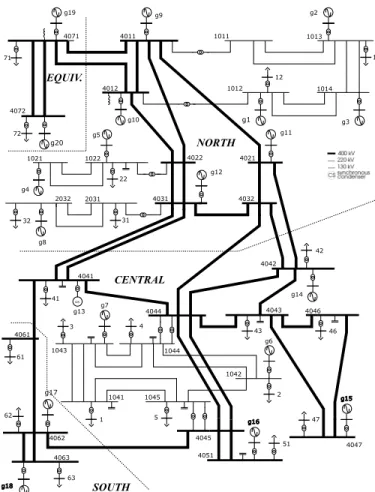
The one-line diagram is given in Fig. 1. The system has rather long transmission lines with 400-kV nominal voltage. Five lines are equipped with series compensation: 4031-4041 (two circuits) by 50%, 4032-4044 by 37.5%, 4032-4042 by 40%, and 4021-4042 by 40%. The model also includes a representation of some regional systems operating at 220 and 130 kV, respectively. All 20 generators (19 synchronous generators and one condenser) are represented behind their step-up transformers, and all 22 loads at distribution level are controlled by the LTCs of the step-down transformers.

This system is made up of the following four areas:

• “North” with hydro generation and some load.

• “Central” with much higher load and thermal power

generation.

• “Equiv” connected to the “North”, which includes a

simple equivalent of an external system.

• “South” with thermal generation, which is rather loosely

connected to the rest of the system.

Table II gives the active power generated and consumed in each area.

All generators were modeled with three or four rotor wind-ings, and saturation. Simple generic models were used for the

g11 g20 g19 g16 g17 g18 g2 g9 g1 g3 g10 g5 g4 g12 g8 g13 g14 g7 g6 g15 4011 4012 1011 1012 1014 1013 1022 1021 2031 cs 4046 4043 4044 4032 4031 4022 4021 4071 4072 4041 1042 1045 1041 4063 4061 1043 1044 4047 4051 4045 4062 NORTH CENTRAL EQUIV. SOUTH 4042 2032 1 5 2 3 4 63 62 61 51 47 42 41 31 32 22 12 13 71 72 46 43

Fig. 1. One-line diagram of the Nordic test system. TABLE II

LOAD AND GENERATION ACTIVE POWERS

area generation (MW) load (MW)

North 4629 1180

Central 2850 6190

South 1590 1390

Equiv 2437 2300

excitation systems, automatic voltage regulators, power system stabilizers, turbines and speed governors. With regarding to long-term dynamics the following modeling considerations were made:

• LTCs act with different delays on the first and subsequent

tap changes, as well as from one transformer to another.

• The OELs of the four smallest generators act after a fixed

time while all the others have inverse-time characteristics, i.e. the higher the field current, the faster its limitation. All loads are connected to LTC-controlled distribution buses, and are modeled as constant current/admittance for the ac-tive/reactive power demand.

Frequency is controlled by the speed governors of the hydro generators in the North and Equiv areas only. The generator g20 is an equivalent generator, with a large participation in primary frequency control. The thermal units of the Central and South areas do not participate in this control. Generator g13 is a synchronous condenser.

The system is heavily loaded with large transfers essentially from the North to the Central areas. Secure system operation is

limited by transient (angle) and long-term voltage instability. The contingencies likely to yield voltage instability are the following:

• The tripping of a line in the North-Central corridor,

forcing the power to flow over the remaining lines.

• The outage of a generator located in the Central area,

compensated by the Northern hydro generators, which adds to the power transfer in the North-Central corridor. The maximum power that can be delivered to the Central loads is strongly influenced by the reactive power capabilities of the Central and some of the Northern generators; their reactive power is limited by OELs. On the other hand, the LTCs aim at restoring distribution voltages and hence load powers. If, after a disturbance (such as a generator or a line outage), the maximum power that can be delivered by the combined generation and transmission system is smaller than what the LTCs attempt to restore, voltage instability results. Thus, this is a long-term instability, driven by OELs and LTCs that takes place in a few minutes minutes after the initiating event. The instability mechanism is similar for demand increases.

B. Operating Points

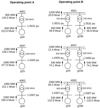
Two operating points are considered. The first one, de-noted A, is insecure, i.e. the system cannot stand some N-1 contingencies. The system is made secure by rather simple modifications of operating point A leading to operating point B. The changes, depicted in Fig. 2, are as follows:

• In parallel with g16, an identical generator (g16b) with

identical step-up transformer is connected, producing the same active power for the same terminal voltage. The additional production of 600 MW is compensated by g20. The power flowing in the North-Central corridor is decreased by almost the same amount, which makes the system significantly more robust.

• For Operating Point B, the system could not withstand the

loss of g15 or g18. Hence, these contingencies are made less severe by replacing each of these generators by two identical generators with half nominal apparent power, half nominal turbine power, and half power output.

IV. SIMULATION RESULTS OFNORDIC TEST SYSTEM

A. Response to a Large Disturbance

In all presented cases, the disturbance is a three-phase solid fault on line 4032-4044, near bus 4032, lasting 5 cycles (0.1 s) and cleared by opening the line, which remains opened. The evolution of two transmission bus voltages is shown Fig. 3 for initial operation at points A and B, respectively.

For operating point A, in response to the initial disturbance, the system undergoes electromechanical oscillations that die out in 20 s. Then, the system settles at a short-term equi-librium, until the LTCs start acting at 35 s. Subsequently, the voltages evolve under the effect of LTCs and OELs. The system is long-term voltage unstable and eventually collapses, less than three minutes after the initiating line outage. As shown in the figure, essentially the Central area is affected;

Operating point A Operating point B

4051 g16 1.0531 pu 600 MW 222.6 Mvar 600 MW 143.5 Mvar 4047 g15 1.0455 pu 1080 MW 1080 MW 228.2 Mvar 4063 g18 1.0307 pu 1060 MW 1060 MW 151.1 Mvar 377.9 Mvar 293.4 Mvar 4051 g16 1.0531 pu 600 MW 59.9 Mvar 1200 MW 20.8 Mvar g16b 600 MW 59.9 Mvar 1.0531 pu 4047 g15 1.0455 pu 540 MW 74.1 Mvar 1080 MW 12.4 Mvar g15b 540 MW 74.1 Mvar 1.0455 pu 4063 g18 1.0307 pu 530 MW 110.5 Mvar 1060 MW 83.2 Mvar g18b 530 MW 110.5 Mvar 1.0307 pu

700 MVA 700 MVA 700 MVA

1200 MVA 600 MVA 600 MVA

600 MVA 600 MVA

1200 MVA

Fig. 2. Main differences between operating points A and B.

0.65 0.7 0.75 0.8 0.85 0.9 0.95 1 1.05 0 20 40 60 80 100 120 140 160 180 t (s)

bus 1041 operating point A: voltage magnitude (pu) bus 4012 operating point A: voltage magnitude (pu) bus 1041 operating point B: voltage magnitude (pu) bus 4012 operating point B: voltage magnitude (pu)

Fig. 3. Evolution of two transmission voltages at operating points A and B.

voltages in other areas are comparatively little influenced. The same figure shows the stable evolution of the same voltages when starting from operating point B.

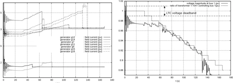
Figure 4 shows the field currents of the seven generators that get limited for initial operating point A. Their OELs act in the order shown in the legend, from top to bottom.

The timing of OEL activation is illustrated in Fig. 5 for two of the seven generators. Under the effect of the fault, the field current of g11 exceeds transiently its limit, then comes back below it; thus, the OEL resets. The field current increases

again after t ≃ 35 s under the effects of LTCs and other

generators getting limited. The field current limit is crossed

again at t≃ 63 s. As the OEL of g11 has a fixed activation

delay of 20 s, it reduces the field current at t≃ 83 s. A similar

evolution is observed for g14, but the field current settles above

the limit sooner, at t≃ 3 s. Unlike g11, the OEL of g14 obeys

2 2.5 3 3.5 0 20 40 60 80 100 120 140 160 180 t (s)

generator g12 : field current (pu) generator g14 : field current (pu) generator g7 : field current (pu) generator g11 : field current (pu) generator g6 : field current (pu) generator g15 : field current (pu) generator g16 : field current (pu)

Fig. 4. Field currents of seven limited generators (oper. point A).

shorter the activation delay) and it acts at t≃ 67 s.

✁✂ ✄ ✄✁✂ ☎ ☎✁✂ ✆ ✆ ✁✂ ✝ ✄ ✝ ✆✝ ✞✝ ✟✝ ✝✝ ✠✡☛ ☞ ✌✍ ✎✏✑✒ ✓✔✔ ✎✕ ✠✏✍ ✖✍✠✗✌✘✆ ✌✍✎✏✑✒✓✔✔ ✎✕✠✏✍✖✍ ✠✗✌✘ ✘ ✎✕ ✎✔ ✙✠✗✔✘ ✚✌✍✎✏✑✒ ✓✔✔ ✎✕ ✠✡✛✓☞ ✘ ✎✕ ✎✔ ✙✠✗✔✘✆✚✌✍✎✏✑✒ ✓✔✔ ✎✕ ✠✡✛✓☞

Fig. 5. Field current evolutions and corresponding limits of two generators. Fig. 6 shows the evolution of the ratio of the transformer connected to bus 1041 and feeding the distribution bus 1, together with the voltage magnitude at that bus. The LTC fails to bring the distribution voltage back within the deadband (also shown in the figure). The distribution voltages, and hence the load powers cannot be restored to their pre-disturbance values, which is typical of long-term voltage instability. The figure also illustrates the multi-dimensional aspect of instability, i.e. interactions between LTCs. Indeed, each tap change brings a proper correction of the distribution voltage but, in between, the same voltage drops more under the effect of the other LTCs acting to restore their own voltages [8], [2].

B. Determination of a Secure Operation Limit

Voltage security is preventively assessed through the deter-mination of a Secure Operating Limit (SOL), which involves stressing the system in its pre-contingency configuration. The stress considered here is an increase of loads in the Central area. The SOL corresponds to the maximum load power that can be accepted in the pre-contingency configuration such that

0.88 0.9 0.92 0.94 0.96 0.98 1 1.02 0 20 40 60 80 100 120 140 160 180 t (s)

voltage magnitude at bus 1 (pu) ratio of transformer 1-1041 controlling bus 1(pu) LTC voltage deadband

Fig. 6. Failed restoration of a distribution voltage by LTC (oper. point A).

the system responds in a stable way to each of the specified contingencies [2]. To this purpose, power flow computations were performed for increasing values of the Central active and reactive loads (in proportion to their base case value, and under constant power factor). For each so determined operating point, the disturbance is simulated. The system response is considered acceptable if, over a simulated time of 600 s: (i) all distribution voltages are restored in their deadbands; (ii) no generator voltage falls below 0.85 pu; and (iii) no loss of synchronism takes place.

In these pre-contingency power flow calculations, the active power variations are compensated by generator g20, while transformer ratios are adjusted as follows: the 22 distribution transformers are adjusted in order to maintain the distribution voltages in the deadbands, while the 400/130-kV transformers 4044-1044 and 4045-1045 (see Fig. 1) are assumed to be controlled by operators, adjusting their ratio to maintain the voltages at buses 1044 and 1045 in specified ranges. The latter transformers do not have their tap changed in the post-disturbance simulation, whose duration is considered too short for operators to react.

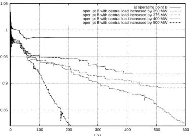
Fig. 7 shows the post-disturbance evolution of the voltage at bus 1041, for various pre-contingency load levels. The case with 375 MW loading seems stable but instability is revealed at about 800 s. Thus, for that contingency, it is safe to set the SOL to 350 MW. Incidentally, the figure illustrates that, in marginal cases, it takes more time for the system to show its stability or instability.

C. Corrective Control by a SIPS

There are several possible control measures to restore stabil-ity. These include LTC blocking [3], tap reversing and voltage setpoint adjustment [11]. An example of SIPS corrective control is given in Fig. 8. The SIPS considered in this example consists of distributed undervoltage load shedding controllers as detailed in [12]. Each controller monitors the voltage at a transmission bus and acts on the load at the nearest distribution bus, according to the following simple rule: “curtail a step ∆P of load active power when the monitored transmission

0.85 0.9 0.95 1 1.05 0 100 200 300 400 500 600 t (s) at operating point B oper. pt B with central load increased by 350 MW oper. pt B with central load increased by 375 MW oper. pt B with central load increased by 400 MW oper. pt B with central load increased by 500 MW

Fig. 7. Evolution of voltage at bus 1041 for various pre-contingency stresses.

voltage V has stayed below a threshold Vth for more than

a time τ ”. Note that each controller can act several times, which yields a closed-loop behavior offering better robustness and adaptiveness. The various controllers do not exchange information but interact through the grid voltages.

0.86 0.88 0.9 0.92 0.94 0.96 0.98 1 1.02 0 50 100 150 200 250 t (s)

voltage magnitude at bus 1041 (pu) with load shedding voltage magnitude at bus 1041 (pu) without load shedding

Fig. 8. Voltage magnitude at bus 1041, with and without load shedding.

The example in Fig. 8 was obtained with Vth= 0.90 pu,

∆P = 50 MW, and τ = 3 s. The load reactive powers were decreased so that their power factors at 1 pu voltage is preserved. A total of 300 MW of load is shed in six steps: two by the controller monitoring bus 1041 and acting on bus 1 (at 100 and 144.95 s), and four by the controller monitoring bus 1044 and acting on bus 4 (at 112.1, 123.1, 180.4, and 290.45 s).

D. PV Curve and Loadability Limit

The last illustrative result deals with PV curves computed to determine the loadability limit of the system (without contingencies). In place of a continuation power flow, the PV curves were obtained by simulating a smooth ramp increase

in demand, not far from what could be observed in a real system. The dynamic response was computed (with a time step size of 0.05 s) with all components active, in particular LTCs and OELs. The simulation was stopped whenever a bus voltage reached an unacceptably low value, or it was ascertained that maximum load power had been crossed. PV curves are obtained by recording the evolutions of voltages and total load power with time, and plotting the former as a function of the latter.

The PV curves in Fig. 9 were obtained starting from operating point B and increasing all loads in the Central area (in proportion to their base case value, and under constant power factor), at a rate of 0.15 MW/s for the whole area. Primary frequency control was relied upon to compensate the power changes. To mimic manual control by operators, the 400/130-kV transformers 4044-1044 and 4045-1045 (see Fig. 1) were also equipped with LTCs adjusting the ratios in steps, with delays, to keep the voltages at buses 1044 and 1045 in pre-specified intervals.

The curves show a loadability limit near 6830 MW, yielding a load power margin of 640 MW. It can be seen that the voltage at bus 1044 is kept almost constant, owing to successive tap changes on transformers 4044-1044. The voltage at bus 1041 is not controlled by an LTC but that bus is electrically close to 1044; hence, its voltage drops a little during the load increase. On the other hand, at the transmission bus 4044, the decline is much more pronounced.

0.95 0.97 0.99 1.01 1.03 1.05 1.07 1.09 1.11 6200 6250 6300 6350 6400 6450 6500 6550 6600 6650 6700 6750 6800 6850 P (MW)

Base Load Level

V (pu)

BUS 1041 (130 kV) BUS 4044 (400 kV) BUS 1044 (130 kV)

Fig. 9. PV curve for load increase in the Central area.

V. OVERVIEW OF THERVS TESTSYSTEM

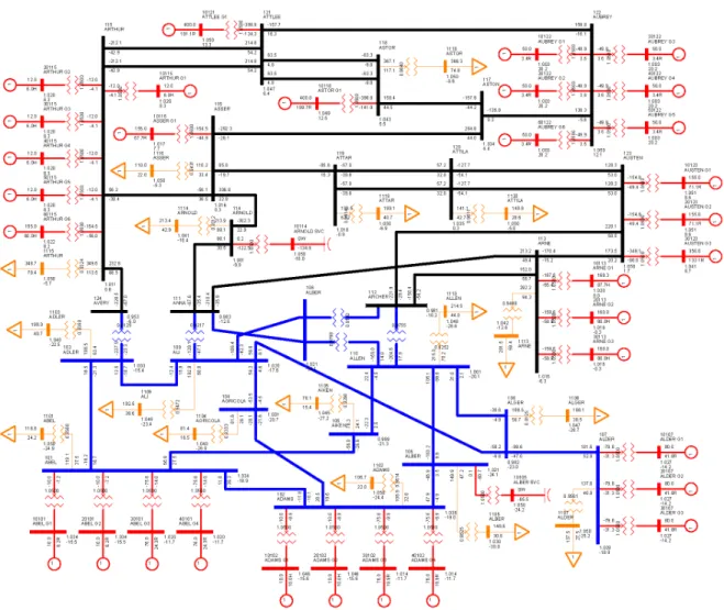
This test system corresponds to a large extent to the 1979 IEEE Reliability Test System [13]. The data presented in the TF report [4] relate to the so-called “one area RTS-96” system [14], which is equivalent to the 1979 Reliability Test System [13]. The one-line diagram of the network is shown in Fig. 10. The original setting of these test systems or their modifi-cations are used to study some aspects of voltage stability. References [15]-[18] present a sample of those works. The parameters of that benchmark system were adjusted to make voltage instability more pronounced. Several modifications

Fig. 10. One-line diagram of the RVS test system.

were also introduced in the power flow data of the original 1979 Reliability Test System, to make again the resulting model more suitable for voltage stability analysis. The main modifications were as follows:

• The synchronous condenser at bus 114 was replaced by

a Static Var Compensator (SVC) with nominal range −50/ + 200 Mvar. As is well known, the reactive power output of this device is voltage dependent and its reactive power output is significantly reduced under low voltage conditions.

• The shunt at bus 106 was replaced by another SVC with

a range of −50/ + 100 Mvar. This change introduces

an additional degree of freedom that is very important for voltage control. This SVC is a key component in the RVS system and is required to avoid voltage instability. Usually the fast response of an SVC is not needed to improve long-term voltage stability. It is used in this sys-tem either with the understanding that it is equivalent to switched capacitor banks, or to improve voltage recovery after fault clearing in the presence of induction motors (see SectionVI-B3).

• The step-up transformers of generators and SVCs are

explicitly represented, assuming five tap positions without LTC. The SVCs control their transmission-side voltages. The power flow solution considers all generators remotely

controlling the voltage at the high-voltage side of their step-up transformers. In the dynamic simulation, all ex-citation systems control the generator terminal voltages.

• All other transformers are represented with LTCs

allow-ing a±10% adjustment of the ratios in 33 steps (0.625%

per step). Each of them is located on the high-voltage side of the transformers and controls the voltage at the distribution (MV) side.

• Loads are no longer connected to the 138- or

230-kV buses. Step-down transformers connecting LTC-controlled 13.8-kV buses were introduced with an es-timated 0.15 pu reactance on an MVA base set to the lowest multiple of 50 MVA greater than 110% of the load apparent power.

• The simulations were performed, initially, with all loads

represented as 100% constant current for the active power and 100% constant impedance for the reactive power components.

• Power recovery and induction motor models were also

included to study the impact of these types of loads in long- and short-term voltage stability phenomenon. In this test system, OELs obey an inverse-time characteristic and act through the main summation point of the AVR. Thus, the OEL output signal is added to the voltage error signal, and can be thought of as a correction added to the voltage

Fig. 11. PV curves for the base case and two contingencies.

reference setpoint. The model and associated parameters are documented in the TF Report. The inverse time characteristic is approximated by a piecewise linear curve defined by three pairs of points relating time and field current.

VI. SIMULATION RESULTS OFRVSTEST SYSTEM

A. Steady-state Analysis

The steady-state analysis starts with the N-1 contingency analysis of all 230-kV and 138-kV circuits. The following 3 contingencies led to non-convergent power flow conditions:

• Outage of the 230-kV circuit between buses 115 and 124.

• Outage of the 138-kV circuit between buses 107 and 108.

• Outage of the 138-kV circuit (cable) between buses 106

and 110.

Voltage stability of a system based on steady-state models is usually examined through its PV curves. The additional generation available at the generator buses to supply the load increase is close to 100 MW; thus, the power transfer increment in PV curve calculations is limited by this amount. The following two contingencies were also considered in PV curve calculations:

• Contingency I: Outage of the 230-kV circuit between

buses 111 and 114.

• Contingency II: Outage of the 230-kV circuit between

buses 112 and 123.

The lines in these contingencies are important links for ex-changing power between 230-kV and 138-kV subsystems. Moreover, for these contingencies, the system does not col-lapse and it is still possible to increase the load and study the system performance.

The PV curves obtained for the two contingencies and the base case are shown in Fig. 11. These plots correspond to the voltage at the load (13.8-kV) bus 1106. Note that Contingency II resulted in a maximum incremental transfer of just 10 MW.

B. Dynamic Responses to Contingencies

The following disturbances were considered in the dynamic simulations:

• Test I: Connecting a 250 Mvar reactor at bus 101 at 0.1 s.

Fig. 12. Response of generator at bus 30101 (Test I).

• Test II: Outage of the cable between buses 106 and 110

without faults.

• Test III: Outage of the cable between buses 106 and 110

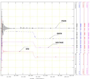
to clear a 3-phase fault at bus 106 after six cycles. 1) Test I: This test corresponds to a 250 Mvar shunt reactor being connected to bus 101 at 0.1 s. Since this is a relatively small disturbance, the voltage at bus 101 drops from the initial value of 1.034 pu to approximately 0.906 pu once the reactor is switched on. This results in the two generators connected to bus 101 (generators 3 and 4 at buses 30101 and 40101) hitting their over-excitation limits.

Fig. 12 presents the response of the generator 3 (bus 30101). It shows the active and reactive power outputs of the machine (in pu of the system base, 100 MVA), terminal voltage, generator field voltage and the output of the OEL. Following the initial disturbance and after transients caused by the disturbance, the generator field current settles at 2.82 pu, higher than the rated field current for this machine (2.473 pu), entering the inverse time characteristic of the OEL model. The OEL model becomes active at approximately 50 s. Since the OEL model represents a summation point OEL action, the OEL starts to lower the voltage reference set-point for the generator, so that terminal voltage and reactive power output are ramped down until a new steady state is reached at lower voltages.

Fig. 13 shows the response of the load connected to bus 101 (13.8-kV bus 1101), where the effect of the on-load tap changers is clearly observed. The initial voltage at bus 1101 is 1.049 pu and, after several steps in the LTC response, it recovers to 1.036 pu. Since voltage recovers to almost the initial value, the load demand recovers to close to its original power demand at the end of the simulation.

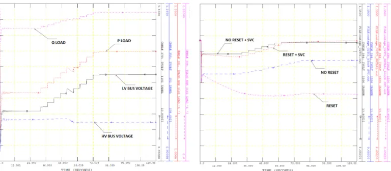
2) Test II: The second simulated disturbance corresponds to Figs. 14 to 16 which present the voltages at buses 106 and 1106, and the active power demand of the load at bus 1106. It is known that aggregate loads, representing the combined

Fig. 13. Response of load at bus 1101 (Test I).

Fig. 14. Voltage at 138 kV bus 106 (Test II).

demand from many consumers, tend to restore their power demand following a disturbance. Thus, it is necessary to represent the load recovery (referred to as RESET in the figures) in long-term dynamic simulations. The RESET model restores the pre-contingency load consumption, to show the effect of restorative loads, such as thermostatically controlled. However, the response rate is artificially increased to speed up simulation. Thus the RESET curves in the figures can be understood as lasting longer. Note that no interaction with other dynamics is introduced by this artificial speed-up.

It can be observed that the dynamic response of the SVC at bus 10106 is critical to avoid a voltage collapse condition around bus 106. In fact, the SVC response combines with the LTC response to bring the voltage at the load bus 1106

Fig. 15. Voltage at 13.8 kV bus 1106 (Test II).

Fig. 16. Active power demand of load at bus 1106 (Test II).

to a higher value than the initial condition. Since the load is modeled with a voltage dependence characteristic, the load demand becomes greater than the initial value and the load recovery model ends up reducing the load demand.

On the other hand, when the SVC is blocked, the voltages at buses 106 and 1106 do not recover. Without the load recovery characteristic, these voltages stabilize at around 0.9 pu due to the associated reduction in active and reactive power demand. When the load recovers to its pre-disturbance power demand, voltages decrease even further and stabilize just above 0.8 pu. Since this is a slow voltage collapse condition, it is con-ceivable that mechanically-switched capacitor banks could be used instead of SVCs.

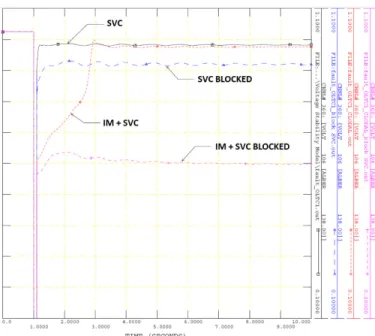
Fig. 17. Voltage at 138 kV bus 106 (Test III).

3) Test III: The third simulated disturbance corresponds to Fig. 17, which present the voltage at bus 106. Once again, the dynamic response of the SVC is critical to avoid a voltage collapse condition around bus 106, caused by the increase in reactive power demand due to stalling induction motors (IM). This is a fast dynamic phenomenon and, in this case, the control capability of the SVC is required to avoid sluggish voltage recovery and the possibility of load disconnection due to sustained low voltages. Further details can be found in [4].

VII. CONCLUSIONS

The TF has provided case studies for education and re-search purposes, in particular to test new solutions for the assessment, detection and mitigation of voltage instability, and for relevant comparisons of methods and software packages. Although relevant, some components and controls were not considered by the TF, mainly because they are less widely used; armature current limiters, control of generator step-up transformer ratios, and secondary voltage control [3] are typical examples. These items could be considered in future extensions together with the models of other important com-ponents such as: alternative OEL models, HVDC links (of both LCC and VSC types), (converter-interfaced) generation dispersed in distribution networks, load dropout, and others.

Since the time of the TF completing its work, the test systems have been used in various research works (e.g. [11]). Furthermore, the models have been extended to cover other dynamic phenomena such as short-term voltage instability, delayed voltage recovery or frequency control. Examples of such studies are easily found on IEEEXplore and in the report of another IEEE TF [19]. Let us quote non exhaus-tively: replacement of a subset of synchronous generators by large-scale photo-voltaic systems for short- and long-term voltage studies, extension of the model into a combined transmission-distribution grid [19], low-frequency oscillations damping using battery energy storage, system reinforcement

through point-to-point HVDC links, incorporation as AC area within a multi-terminal DC grid, addition of a communication infrastructure for cyber-physical security studies, frequency stability in the presence of large-scale wind farms.

The Power System Community is herein heartily encour-aged to contribute to these updates by sharing the relevant documentation and data files. This update activity is being supported by the Working Group on Dynamic Security Assess-ment sponsored by the Power System Stability Subcommittee of the Power System Dynamic Performance Committee.

REFERENCES

[1] C. W. Taylor, Power System Voltage Stability, EPRI Power System Engineering Series, McGraw Hill, 1994.

[2] T. Van Cutsem, C. Vournas, Voltage stability of electric power systems, Springer (previously Kluwer Academic Publishers), Boston (USA), 1998.

[3] S. Corsi, Voltage Control and Protection in Electrical Power Systems, Springer, 2015.

[4] T. Van Cutsem (Chair) et al., “Test systems for voltage stability analysis and security assessment,” IEEE/PES Power System Stability

Subcommittee, Tech. Rep. PES-TR19, Aug. 2015.

[5] C. Ca˜nizares (Editor) et al. “Voltage stability assessment: concepts, practices and tools,” IEEE/PES Power System Stability Subcommittee, Tech. Rep. PES-TR9, Aug. 2002.

[6] P. Kundur, Power system Stability and Control, EPRI Power System Engineering Series, McGraw Hill, 1994, pp. 337-339.

[7] M. Stubbe (Convener), Long-term dynamics - phase II, Report of CIGRE Task Force 38.02.08, Jan. 1995.

[8] C. Vournas, T. Van Cutsem, “Local identification of voltage emergency situations,” IEEE Trans. on Power Systems, vol. 23, no 3, pp. 1239-248, Aug. 2008.

[9] M. Glavic, T. Van Cutsem, “Wide-area detection of voltage instability from synchronized phasor measurements. part I: principle. part II: simulation results,” IEEE Trans. on Power Systems, vol. 24, no. 3, pp. 1408-1425, Aug. 2009.

[10] M. Glavic, M. Hajian, W. Rosehart, and T. Van Cutsem, “Receding-horizon multi-step optimization to correct nonviable or unstable trans-mission voltages,” IEEE Trans. on Power Systems, vol. 26, no. 3, pp. 1641-1650, Aug. 2011.

[11] C. D. Vournas, C. Lambrou, and M. Kanatas, “Application of local autonomous protection against voltage instability to IEEE test system,”

IEEE Trans. on Power Systems, vol. 31, no. 4, pp. 3300-3308, Jul. 2016.

[12] B. Otomega, M. Glavic, T. Van Cutsem, ‘Distributed undervoltage load shedding,” IEEE Trans. on Power Systems, vol. 22, no 4, pp. 2283-2284, Nov. 2007.

[13] Reliability Test System Task Force of the Application of Probability Methods Subcommittee, “IEEE reliability test system,” IEEE Trans. on

PAS, vol. 98, no. 6, pp. 2047-2054, Nov./Dec. 1979.

[14] Reliability Test System Task Force of the Application of Probability Methods Subcommittee, “The IEEE reliability test system-1996,” IEEE

Trans. on Power Systems, vol. 14, no. 3, pp. 1010-1020, Aug. 1999.

[15] R. Billinton, S. Aboreshaid, “Voltage stability considerations in compos-ite power system reliability evaluation,” IEEE Trans. on Power Systems, vol. 13, no. 2, pp. 655-660, May 1998.

[16] J. A. Momoh, Y. V. Makarov, W. Mittelstadt, “A framework of voltage stability assessment in power system reliability analysis,” IEEE Trans.

on Power Systems, vol. 14, no. 2, pp. 484-491, May 1999.

[17] H. Wan, J. D. McCalley, V. Vittal, “Risk based voltage security assess-ment,” IEEE Trans. on Power Systems, vol. 15, no. 4, pp. 1247-1254, Nov. 2000.

[18] A. B. Rodrigues, R. B. Prada, M. D. G. da Silva, “Voltage stability probabilistic assessment in composite systems: modeling unsolvability and controllability loss,” IEEE Trans. on Power Systems, vol. 25, no. 3, pp. 1575-1588, Aug. 2010.

[19] N. Hatziargyriou (Chair) et al. “Contribution to Bulk System Control and Stability by Distributed Energy Resources connected at Distribution Network,” IEEE/PES Power System Stability Subcommittee, Tech. Rep. PES-TR22, Jan 2017