HAL Id: hal-01576133
https://hal.inria.fr/hal-01576133
Submitted on 22 Aug 2017
HAL is a multi-disciplinary open access
archive for the deposit and dissemination of
sci-entific research documents, whether they are
pub-lished or not. The documents may come from
teaching and research institutions in France or
abroad, or from public or private research centers.
L’archive ouverte pluridisciplinaire HAL, est
destinée au dépôt et à la diffusion de documents
scientifiques de niveau recherche, publiés ou non,
émanant des établissements d’enseignement et de
recherche français ou étrangers, des laboratoires
publics ou privés.
Minnie : An SDN world with few compressed forwarding
rules
Myriana Rifai, Nicolas Huin, Christelle Caillouet, Frédéric Giroire, Joanna
Moulierac, Dino Lopez Pacheco, Guillaume Urvoy-Keller
To cite this version:
Myriana Rifai, Nicolas Huin, Christelle Caillouet, Frédéric Giroire, Joanna Moulierac, et al.. Minnie :
An SDN world with few compressed forwarding rules. Computer Networks, Elsevier, 2017, 121, pp.185
- 207. �10.1016/j.comnet.2017.04.026�. �hal-01576133�
Procedia Computer Science 00 (2017) 1–34
Procedia
Computer
Science
M
INNIE
: an SDN World with Few Compressed Forwarding Rules
Myriana Rifai
a, Nicolas Huin
a,b, Christelle Caillouet
a,b, Frederic Giroire
a,b, Joanna
Moulierac
a,b, Dino Lopez Pacheco
a, Guillaume Urvoy-Keller
aaUniversit´e Cˆote d’Azur, CNRS, I3S, UMR 7271, 06900 Sophia Antipolis, France bInria Sophia Antipolis
Abstract
Software Defined Networking (SDN) is gaining momentum with the support of major manufacturers. While it brings flexibility to the management of flows within the data center fabric, this flexibility comes at the cost of smaller routing table capacities. Indeed, the Ternary Content-Addressable Memory (TCAM) needed by SDN devices has smaller capacities than CAMs used in legacy hardware.
In this paper, we investigate compression techniques to maximize the utility of SDN switches forwarding tables. We validate
our algorithm, called MINNIE, with intensive simulations for well-known data center topologies, to study its efficiency and
com-pression ratio for a large number of forwarding rules. Our results indicate that MINNIEscales well, being able to deal with around
a million of different flows with less than 1000 forwarding entries per SDN switch, requiring negligible computation time.
To assess the operational viability of MINNIEin real networks, we deployed a testbed able to emulate a k= 4 Fat-Tree data
center topology. We demonstrate on the one hand, that even with a small number of clients, the limit in terms of number of rules
is reached if no compression is performed, increasing the delay of new incoming flows. MINNIE, on the other hand, reduces
drastically the number of rules that need to be stored, with no packet losses, nor detectable extra delays if routing lookups are done in the Application-Specific Integrated Circuits (ASICs).
Hence, both simulations and experimental results suggest that MINNIEcan be safely deployed in real networks, providing
compression ratios between 70% and 99%.
Keywords: Software Defined Networks, data center networks, routing tables, compression, TCAM
1. Introduction
In classical networks, routers compute routes using distributed routing protocols such as OSPF (Open Shortest Path First) [1] to decide on which interfaces packets should be forwarded. In SDN (Software Defined Network), one or several controllers take care of route computations and routers become simple forwarding devices. When a packet arrives with a new destination for which no routing rule exists, the router1contacts a controller that provides a route to the destination. Then, the router stores this route as a rule in its SDN table and uses it for next incoming matching packets. This separation of the control plane from the data plane allows a smoother control over routing and an easier management of the routers.
Also, SDNs aim at applying flow-based forwarding rules instead of destination-based rules (as in legacy routers) to provide a finer control of the network traffic. For instance, in OpenFlow 1.02, forwarding decisions can be made taking into account from zero up to a maximum of 12 fields of a TCP or UDP packet. When any of the 12 fields should be ignored when forwarding a packet, such a field is set to “don’t care bits”. Due to the complexity of SDN forwarding rules, SDN forwarding devices need TCAMs (Ternary Content-Addressable Memories) to store their routing table (as classical CAM can only perform binary operations). However, TCAMs are more power hungry, expensive and physically bigger than binary CAMs available in legacy routers. Consequently, the available TCAM memory in routers is limited. Indeed, a typical switch supports between around a couple of thousands to no more than 25 thousands of 12-tuples forwarding rules, as reported in [2].
Undoubtedly, emerging switches will support larger forwarding tables [3], but TCAMs still introduce a funda-mental trade-off between forwarding table size and other concerns like cost and power. The maximum size of routing tables is thus limited and represents an important concern for the deployment of SDN technologies. This problem has been addressed in previous works, as discussed in Section 2, using different strategies, such as routing table compression [4, 5], or distribution of forwarding rules [6].
In this work, we examine a more general framework in which table compression using wildcard rules is possible. Compression of SDN rules was discussed in [4]. The authors propose algorithms to reduce the size of the tables, but only by using a default rule. We consider here a stronger compression methodology in which any packet header field may be compressed. Considering multiple field aggregation is an important improvement as it allows a more efficient compression of routing tables, leaving more space in the TCAM to apply advanced routing policies, like load-balancing and/or to implement quality of service policies. In the following, we focus on compression of rules based on sources and destinations. However, our solution also applies if other fields are considered, such as ToS (Type of Service) field or transport protocol.
We consider the problem, formally defined in Section 3, of routing a set of flows with a limited number of SDN rules using compression. The problem is NP-complete, as even compressing a single multifield table is NP-complete (even for two fields), see [7].
A short version of this work has been presented in [8]. In our previous publication, we presented our any-field compression approach and provided a brief description of our compression algorithm and preliminary results about its compression and scalability properties. However, the previous proposition lacked compression capabilities at the access switches, reducing its usability spectrum, which is not the case of the solution provided in the present document. Moreover, in [8] we only considered Fat-Trees topologies with only 128 servers and low bandwidth rates.
In this paper, we complement our previous work by compressing on all switches and extending our experiment’s spectrum. In brief, our added contributions are the following:
- We provide a detailed description of our compression algorithm, MINNIE, in Section 3, which routes the traffic and compresses routing tables to satisfy link capacity and routing table size constraints of the different forward-ing devices. The compression can be done on different flow fields allowforward-ing advanced routforward-ing policies.
- Routing is done dynamically, meaning that routing and compression decisions are taken online when a new flow arrives. We show that compressing tables at the right moment can lead to significant gains in Section 4.2.
1In the following, we make no distinction between routers/switches, packets/frames and routing/forwarding tables using these terms in their
general sense.
2https://www.opennetworking.org/images/stories/downloads/sdn-resources/onf-specifications/
openflow/openflow-spec-v1.0.0.pdf
Compression Compression Rule # Delay Execution time of MINNIE Additional
ratio frequency on packets in average (ms) results
Simulations
Section 4.2.3 Routing Compression Comparison
Section 4.2.2 Section 4.2.2 Figure 4 Section 4.2.6 Sec. 4.2.6 with XPath Figure 2 Figure 3 Section 4.2.4 Figure 5a Figure 5b Section 4.2.5
Table 3 Figure 6 Table 4
Experiments
First Subsequent Compression
Scenario 1 (LLS) Table 6 Table 7 Table 5 Figure 12 Figure 14 Figure 10 SDN control path
Section 5.2.1 Figure 9 Figure 13 Figure 15 Sec. 5.2.1 Fig. 11
Software
Scenario 2 (HLS) Table 8 Figure 17 Figure 16a Figure 16b vs. hardware
Section 5.2.2 Figure 18 Sec. 5.2.3 Fig. 19
Table 1: Summary of the obtained results in the different sections.
- We first validate the algorithm by extensive simulations on several well-known data center topologies described in Section 4. We demonstrate that MINNIEscales well and can deal with around a million of different flows with less than 1000 entries in the routing tables and with negligible compression time.
- We further validate MINNIEwith a testbed composed of a high-end SDN-capable dedicated router - HP5412zl SDN switch -(referred to as a hardware router in this document) , described in Section 5.1.1. We study different metrics, namely the delay introduced by the communications with the controller, the potential increase of loss rate due to handling of dynamic routing and compression, and the load of the controller with and without compression.
- Our results (Section 5.2) show that MINNIEis able to minimize the number of entries in the switches, while successfully handling client’s dynamics and maintaining network stability.
- Section 6 summarizes the results obtained via simulation and with our testbed and discusses extensions to our solution.
A table of contents of the results obtained through simulations and experiments is presented in Table 1.
2. Related work
To support a vast range of network applications, SDN has been designed to apply flow-based rules, which are more complex than destination-based rules in traditional IP routers. As explained in the previous section, the complexity of the forwarding rules are well supported by TCAMs. However, as TCAMs are expensive and power-hungry, the on-chip TCAM size is typically limited.
Many existing studies in the literature have addressed this limited rule space problem. For instance, the authors in [9] and [10] try to compact the rules by reducing the number of bits describing a flow within the switch by inserting a small tag in the packet header. This solution is complementary to ours, however, it requires a change in: (i) packet headers and (ii) in the way the SDN tables are populated. Also, adding an identifier to each incoming packet is hard to be done in the ASICs (Application-Specific Integrated Circuits) since this is not a standard operation, causing the packets to be processed by the central CPU of the router (a.k.a. the slow-path) strongly penalizing the performance and the traffic rate. Another approach is to compress policies on a single switch. For example, the authors in [11, 12, 13] have proposed algorithms to reduce the number of rules required to realize policies on a single switch.
Several works have proposed solutions to distribute forwarding policies while managing rule-space constraints at each switch [6, 14, 15, 16, 17]. However, no compression mechanisms are added to those solutions. For example, in [16], the authors propose OFFICER. It creates a default path for all communications, and later, some deviations are introduced from this path using different policies to reach the destination. According to the authors, the Edge First (EF) strategy, where the deviation is performed to minimize the number of hops between the default path and the target one, offers the best trade-off between the required Quality of Service (QoS) and forwarding table size. Note however, that applying this algorithm could unnecessarily penalize the QoS of flows when the routers’ forwarding tables are rarely full. In [17], the authors propose CacheFlow which introduces a CacheMaster module and a shared section of software switches per TCAM (available in hardware switches only). The CacheMaster constructs the dependency
tree of the rules to be installed and then distributes the rules between the TCAM and the software switches, placing the most popular rules in the hardware switch, thus enabling fast forwarding for the biggest possible amount of traffic. When a packet needs a forwarding rule not available in the TCAM, such a packet is forwarded to the software switches, which send back the packet to the hardware switch in a predetermined input port, to be resent at a specific output port. If the software switches do not have a matching rule, the SDN controller is called. The weaknesses of CacheFlow relies in its inherent architecture, as this solution requires the installation of a software switch for every hardware switch, which might need a reorganization of the network cabling and additional resources to host software switches. Secondly, the optimal number of needed software switches can be difficult to determine, due to the fact that for performance reasons, software switches must only keep forwarding rules (whose number depends on the traffic characteristics) in the kernel memory space, which is limited. Lastly, the two-layer architecture of CacheFlow (i.e. software switches over a hardware switch) increases the delay to contact the controller and install missing rules.
To the best of our knowledge, the closest papers to our work are [5, 18, 4]. In [5] the authors introduce XPath which identifies end-to-end paths using path ID and then compresses all the rules and pre-install the necessary rules into the TCAM. We compare our results with the ones of XPath in Section 4.2.5. MINNIEuses fewer rules even in the case of an all-to-all traffic as XPath codes the routes for all shortest paths between sources and destinations. This is at the cost of less path redundancy which is useful for load-balancing and fault tolerance. Network operators should consider this trade-off when choosing which method to use. In [18] the authors suggest SDN rule compression by following the concept of longest prefix matching with priorities using the Espresso [19] heuristic and show that their algorithm leads to 17% savings only. We succeed in reaching better compression ratios using MINNIE. Last, [4] addresses the problem of compressing routing tables using default rule only in case of Energy-Aware Routing. We extend this solution by considering other types of compression.
3. Modeling of the problem and description of MINNIEalgorithm
We represent the network as a directed graph G= (V, A). A vertex is a router and an arc represents a link between two routers. Each router u has a maximum rule space capacity Sugiven by the size of its routing table and expressed in number of rules. Each link (u, v) ∈ A has a maximum capacity Cuv. A flow is a identified as a triplet (s, t, d), in which s ∈ V is the source of the flow, t ∈ V its destination, and d ∈ R+, its load.
We define a routing rule as a triplet (s, t, p) where s is the source of the flow, t its destination and p the outgoing port of the router for this flow. To aggregate the different rules, we use wildcard rules that can merge rules by source (i.e., (s, ∗, p)), by destination (i.e., (∗, t, p)) or both (i.e., (∗, ∗, p), the default rule). Table 2 shows an example of a routing table and its compressed version using different strategies. Table 2(a) gives the routing table without compression, Table 2(d) the table using default port compression and Table 2(e) the minimal routing table using a mix of compressions by sources and by destinations.
Note that, as we are doing multifield compression, a flow may match several rules. As an example, in the solution with the minimum number of rules (Table 2(e)), the flow (1, 4) is matched both by the rule (1, ∗, 6) and the rule (∗, 4, 4) in the table. We thus have to ensure that a flow is matched by the right rule. To this end, the rules are ordered in the table in the order of decreasing priority. For example, the rule (1, ∗, 6) is placed in the table with a higher priority than rule (∗, 4, 4). This way, the flow (1, 4) is routed through Port-6, which is coherent with the routing of the table without compression Table 2(a). We discuss in Section 5.1.6 how to implement the priorities in practice.
Problem. Given a set of flows D, the problem we consider is to find sets of routing rules (aggregated or not) such that each flow is well routed from its source to its destination while respecting thelink capacity constraints and the table size constraints.
To solve the problem, we propose an algorithm called MINNIE. MINNIE is composed of two modules: the compression module which compresses the routing tables using wildcard rules, and the routing module which finds paths (and routing rules) for the flows using a shortest-path algorithm with an adaptive metrics to spread flows over the network and to avoid overloading a link or a table.
MINNIE, presented in Algorithm 1, works as follows. For every flow to be routed, MINNIE iteratively finds a path using the routing module described in Algorithm 3 (Algo 1, line 4). For every node in the path, it then adds a forwarding rule if no matching wildcard rule already exists. MINNIE calls the compression module, described in
Flow Output port (0, 4) Port-4 (0, 5) Port-5 (0, 6) Port-5 (1, 4) Port-6 (1, 5) Port-4 (1, 6) Port-6 (2, 4) Port-4 (2, 5) Port-5 (2, 6) Port-6
(a) Without Compression
Flow Output port (0, 4) Port-4 (1, 5) Port-4 (2, 4) Port-4 (2, 5) Port-5 (0, ∗) Port-5 (∗, ∗) Port-6
(b) MINNIE: Source table
Flow Output port (1, 4) Port-6 (1, 5) Port-4 (0, 6) Port-5 (∗, 4) Port-4 (∗, 5) Port-5 (∗, ∗) Port-6
(c) MINNIE: Destination table
Flow Output port (0, 5) Port-5 (0, 6) Port-5 (1, 4) Port-6 (1, 6) Port-6 (2, 5) Port-5 (2, 6) Port-6 (∗, ∗) Port-4
(d) MINNIE: Default only
Flow Output port (1, 5) Port-4 (2, 6) Port-6 (1, ∗) Port-6 (∗, 4) Port-4 (∗, ∗) Port-5
(e) Optimal solution (ILP)
Table 2: Examples of routing tables: (a) without compression, (b) compression by the source, (c) compression by the destination, (d) default rule only, and (e) routing table with minimum number of rules given by Integer Linear Program. The order of the rules reads top to bottom.
Algorithm 2, on any table that reached its rule space capacity (Algo 1line 10). We refer to this table compression as a compression event. The total load of flows on each link of the path is then updated to account for the new flow (Algo 1, line 10). We now provide more details about the compression and routing modules.
Algorithm 1: MINNIE Algorithm Input: A digraph G= (V, A) link capacity Cuv, ∀(u, v) ∈ A rule space capacity Su, ∀u ∈ V a set of flows D
Output: a path (with the corresponding rules) for all flows in D 1 flow Fuv= 0, ∀(u, v) ∈ A;
2 set of rules Ru= ∅, ∀u ∈ V; 3 foreach (s, t, d) ∈ D do
4 Find path Pstbetween s and t using Algorithm 3 ; 5 foreach (u, v) ∈ Pstdo
6 if (∗, t, pv), (s, ∗, pv), (∗, ∗, pv) < Ruthen 7 add (s, t, pv) at the top of Ru 8 if |Ru|== Suthen
9 Compress Ruusing Algorithm 2;
10 Fuv= Fuv+ d
3.1. MINNIE: compression module
Since the compression of a single table is NP-Hard [20], we use the following greedy algorithm (Algorithm 2). It first computes three compressed routing tables (aggregation by source (line 1-22), by destination (line 23-44) and by the default rule (line 45-52)) and then chooses the smallest one, as explained in more details below. The theoretical basis of this algorithm was studied in [20] and was proved to be efficient, as it provides a 3-approximation of the compression problem. We show in this paper that it is also efficient in practice.
Given a routing table such as the one given in Table 2(a), the algorithm first considers an aggregation by source (Table 2(b)) using (s, ∗, p∗
s) rules. The main principle is simple, but there is a small technicality to break ties. We first consider the sources one by one and choose (one of) the most occuring port(s) in the rules with this source. It corresponds to the port allowing to compress the most rules using a rule of aggregation by source. Then, we use the default rule to reduce the number of aggregated rules.
There is a small technicality to break ties, when there are several most occurring ports. As a matter of fact, the choice taken of aggregation ports for each source affects the default port chosen. We thus postpone the choice of
the source aggregation port in case of ties in order to choose the default port compressing the largest number of aggregation rules, as explained in details below.
For each source s, we need to find the port p∗
ssuch that we can aggregate using the rule (s, ∗, p∗s), and the port p∗ to aggregate with the default rule (∗, ∗, p∗). First, we compute the set of most occurring ports for each source s, noted P∗
s. The default port p∗is thus the most occurring port in all sets P∗s. If multiple ports can be chosen, one is selected at random. Then, for each source s, the port p∗
sis equal to p∗if p∗∈ P∗s. Otherwise we choose at random among P∗s. Once the ports for the aggregated rules are chosen, we build the compressed table. First, we add rules that cannot be aggregated (line 12), i.e., (s, t, p , p∗
s). Then, we add all the aggregation rules by source that do not use the default port p∗ (line 15), i.e., (s, ∗, p∗s , p∗). Finally, we add the default rule (∗, ∗, p∗) (line 16). The order of insertion in the routing gives the order for the matching, i.e., non aggregated rules, then source aggregation rules and then default rule.
For example, the sets of the most occurring ports of sources 0, 1, and 2 in Table 2(a) are {Port-5}, {Port-6}, {Port-4, Port-5, Port-6}, respectively. Since Port-5 and Port-6 appear two times each, we choose at random Port-6 to be the default port. The ports used for the aggregation by source for 0, 1, 2 are then Port-5, Port-6, Port-6, respectively. Port-6 is chosen for the source 2, because it is the default port. We can now build the compressed table by adding all rules that have ports different than their corresponding aggregate rules: (0, 4, 4), (1, 5, 4), (2, 4, 4), (2, 5, 5). Then, we add all aggregate rules with a port different from the default port: (0, ∗, 5). Finally, we add the default rule (∗, ∗, 5). This gives us the compressed table in Table 2(b).
For the second compressed routing table (Table 2(c)), we do the same compression considering the aggregation by destination with (∗, t, p∗
t) rules. As for the third table (Table 2(d)) a single aggregation using the best default port is performed, i.e., one of the most occurring port in the routing table becomes the default port (tie broken uniformly at random). We then choose the smallest routing table among the three computed ones.
3.2. MINNIE: routing module
We propose an efficient routing heuristics using a weighted shortest-path algorithm with an adaptive metrics. When several routes are possible for a flow, we select the one using the less loaded equipments, links and routers, as measured by our metrics. The intuition is two-fold:(i) we want to avoid sending new flows to a router with a very loaded routing table, if there exists an alternative path using routers with less loaded routing tables (ii) load balancing the traffic over the multiple possible paths is currently done in data centers to avoid overloading links.
For every flow (s, t, d), we first build a weighted directed graph (digraph) Gst = (V, Ast, w), where, for every (u, v) ∈ Ast, wuv is the weight of link (u, v). Gst represents the residual network after having routed the previously routed flows:
- Gst is a subgraph of G where an arc (u, v) is removed if its capacity is less than d or if the flow table of the router u is full and does not contain any wildcard rule for (s, t, pv) (where pv represents the output port of u towards v). Note that, when a table is full and compressed, a node u has only one outgoing arc (to the node v), corresponding to the first existing rule of the form (s, ∗, pv), (∗, t, pv) or to the default rule (∗, ∗, pv). As more tables get full, the number of nodes with only one outgoing arc increases, reducing the size of the graph. - The weight wuvof a link depends on the overall flow load on the link and the table’s usage of router u. We note
wc
uvthe weight corresponding to the link capacity and wruvthe weight corresponding to the rule capacity. They are defined as follows:
wcuv= Fuv Cuv
where Cuvis the capacity of the link (u, v) and Fuvthe total flow load on (u, v). The more the link is used, the heavier the weight is, which favors the use of lower loaded links allowing load-balancing. And
wruv= |Ru|
Su if @ wildcard rule for (s, t, v)
0 otherwise
where Ru is the current set of rules for router u. Recall that Su is the maximum number of rules which can be installed in the routing table of router u. The weight is proportional to the usage of the table. Note that wc
uv∈ [0, 1] and wruv∈ [0, 1]. They measure the percentages of usage of link uv and the routing table of router u. 6
Algorithm 2: Compressing a table Input: Set of rules R
Output: Compressed rules // Compression by source
1 list of rules Cr// order of insertion = order of matching
2 foreach s ∈ V do
3 P∗
s, set of most occurring ports p in {(s, t, p) | ∀t ∈ V};
4 p∗= most occurring port in all P∗s// ties are broken at random
5 foreach s ∈ V do 6 if p∗∈ P∗sthen 7 p∗ s = p ∗ 8 else 9 p∗
s= most occurring port in P
∗
s// ties are broken at random
10 foreach (s, t, p) ∈ R do 11 if p , p∗sthen 12 add (s, t, p) to Cr; 13 foreach s ∈ V do 14 if p∗s, p∗then 15 add (s, ∗, p∗s) to Cr; 16 add (∗, ∗, p) to Cr; // Compression by destination
17 list of rules Cc// order of insertion = order of matching
18 P∗t, set of most occurring ports p in {(s, t, p) | ∀t ∈ V}, ∀s ∈ V;
19 p∗= most occurring port in P∗
t // ties are broken at random
20 foreach t ∈ V do
21 if d ∈ P∗t then
22 p∗t = p∗ 23 else
24 p∗t = most occurring port in P∗t // ties are broke at random
25 foreach (s, t, p) ∈ R do 26 if p , p∗t then 27 add (s, t, p) to Cc; 28 foreach t ∈ V do 29 if p∗t , p∗then 30 add (s, ∗, p∗ t) to Cc; 31 add (∗, ∗, d) to Cc;
// Default port compression
32 list of rules Cd;
33 p∗= most occurring port in R // ties are broke at random
34 foreach (s, t, p) ∈ R do
35 if p , p∗then
36 add (s, t, p) to Cd;
37 add {(∗, ∗, p∗)} to Cd;
38 return smallest set of rules between Cr, Cc, and Cd
The weight wuvof a link (u, v) is then given by:
wuv= 1 + 0.5 wcuv+ 0.5 w r uv.
The additive term 1 is used to provide the shortest path in terms of number of hops when links and routers are not used (i.e., when wcuv = 0 and wruv = 0 for all (u, v) ∈ Ast). This term could be replaced by the delay to traverse link (u, v) to obtain the shortest paths in terms of delay. When the links and routers are used, we take into account their usage. Moreover, we wanted to give the same importance to network link load and table load. Thus, we choose an equal weight of 0.5 for wc
uvand wruv. Note that wuv≤ 2. This ensures that l(p) ≤ 2 × l(p∗), where p is the path found by the routing module, p∗is the unweighted shortest path and l(p) the number of hops of path p (indeed, l(p) ≤ w(p) as wuv≥ 1, w(p) ≤ w(p∗) as p was selected, and w(p∗) ≤ 2 l(p∗), where w(p) is the sum of the weights of the links of path p). This means that no path longer than twice the current available shortest path is selected.
When (Gst, w) is built, we compute a route for the flow by finding a shortest path between s and t in the digraph minimizing the weight w.
Algorithm 3: Finding a path for a flow Input: A flow (s, t, d),
a digraph G= (V, A),
rule space capacity Su∀u ∈ N, set of rules Ru∀u ∈ N, link capacity Cuv∀a ∈ A, flow Fuv, ∀a ∈ A
Output: A path for (s, t, d)
1 Create a weighted digraph Gst= (V, Ast= ∅, W); 2 foreach (u, v) ∈ A do
3 if Cuv− Fuv≥ dthen
4 if ∃ wildcard rule for (s, t, pv) then
5 add edge (u, v) to Gst;
6 wruv= 0;
7 wcuv= Fuv/Cuv;
8 Wuv= 1 + 0.5wruv+ 0.5wcuv; 9 else if |Ru|< Suthen
10 add edge (u, v) to Gst;
11 wruv= |Su|/Ru; 12 wcuv= Fuv/Cuv;
13 Wuv= 1 + 0.5wruv+ 0.5wcuv;
14 return weighted shortest path between s and t in Gst= (V, A0, W)
In the current version of MINNIE, when the algorithm can no longer compress a table, it uses the default action to forward the new traffic to the controller. This could be enhanced to evict the least recently used rule from the table. It should be noted that based on our results (Section 4.2) all flows can be forwarded using a rule space capacity of 1000 rules. Thus, using advanced eviction rules seems unnecessary.
4. Simulations on data center topologies
In this section, we study the behavior of MINNIEthrough simulations for a wide variety of data center architec-tures. We first present the different scenarios, performance metrics and data center architectures in Section 4.1. We then demonstrate that MINNIEworks well for topologies of different sizes and structures in Section 4.2. A table of content of the results obtained through simulations and experiments is available in Table 1.
4.1. Simulation settings
We present in this section the different scenarios studied via simulations, the traffic patterns and metrics that will be evaluated. All simulations were carried out on a computer equipped with a 3.2GHz 8 Core Intel Xeon CPU and 64 GB of RAM.
4.1.1. Scenarios
We ran simulations under three different scenarios:
• Scenario 1: No compression. We only use the routing module of MINNIEand fill up the routing tables without compressing them. This scenario serves as a baseline for measuring the efficiency of MINNIE.
• Scenario 2: Compression at the end of the simulation. We compress the routing tables of every switch once at the end of the simulation, when all the forwarding rules have been stored assuming an unlimited capacity of the routing table. We use it to test the efficiency of the compression module of MINNIE.
• Scenario 3: MINNIE(Dynamic compression at a fixed threshold). We validate MINNIEwith a threshold of 1000 rules, which represents the routing table limit. This scenario aims at testing MINNIEin a scenario closer
to real life. The capacity of 1000 rules has been chosen as it corresponds to the number of entries supported by the TCAM of typical switches such as Apollo 2 and Triumph 2 [21]. The actual number ranges around couple of thousands to tens of thousands [2].
4.1.2. Traffic patterns
For all scenarios, we consider an all-to-all traffic in which every single server establishes a connection to all other servers. Each flow is constantly sending traffic. We consider this situation to test MINNIEin the most extreme scenario in terms of number of flows, and thus, in terms of number of rules. Each flow is represented by a unique source-destination pair.
4.1.3. Data center architectures
To test the efficiency of MINNIE, we considered state-of-the-art data center architectures: Fat-Tree [22], VL2 [23], BCube [24] and DCell [25]. For each family of architecture, we considered topologies of different sizes hosting from few units to about 3000 end points. These end points can be either servers or IP subnets, grouping thousands of different machines. In the following, for simplicity, we often use the term server for both cases. The number of flows routed in the topologies can thus reach a few millions.
The architectures considered during these simulations can be classified into two different groups: • Group 1, in which servers only act as end hosts includes Fat-Tree and VL2.
• Group 2, in which servers also act as forwarding devices (similarly to switches) includes BCube and DCell. We detail below how we chose the different set of parameters to build these topologies like the number of switches or level of recursion.
Fat-Tree. The Fat-Tree is one of the most well-known architectures. The switches are divided into three categories: core, aggregation and access (or ToR for Top of the Rack) switches. A k Fat-Tree is composed of k pods of k switches and k2/4 core switches. Every switch possesses k ports. Inside a pod, aggregation and edge switches form a complete bipartite graph. Each core switch is connected to every pod via one of the k/2 aggregation switches. Every ToR switch has a rack composed of k/2 servers. A k= 4 Fat-Tree is shown as example in Figure 1a.
For our simulations, to build Fat-Trees with up to 3000 servers, we considered k values between 4 and 22. VL2. The VL2 architecture is also composed of three layers of switches: intermediate, aggregation and ToR switches. The intermediate and aggregation switches are connected together to form a complete bipartite graph. Each ToR is connected to two different aggregation switches. Three parameters control the number of switches of each layer and the number of servers of the architecture: Darepresents the number of ports of an aggregation switch, Dithe number of ports of an intermediate switch and T the number of servers in the rack of a ToR switch. Figure 1b shows a
Core
Aggregation Access
(a) Group 1: A Fat-Tree with k= 4 pods
Intermediate
Aggregation ToR
(b) Group 1: A VL2 network with Di =
6-ports intermediate swiches, Da= 6-ports
ag-gregation switches and T= 2 servers per ToR
Dcell(2, 0)[0]
Dcell(2, 0)[1] Dcell(2, 0)[2]
(c) Group 2: A DCell(2, 1), composed of 3 DCell(2,0)
BCube(3, 0)[0] BCube(3, 0)[1] BCube(3, 0)[2]
(d) Group 2: A BCube(3, 1), composed of 3 BCube(3, 0)
Figure 1: Example of topologies studied.
V L2(Da = 6, Di = 6, T = 2). The topology has Da/2 (3 in the example) aggregation switches, Di(6 in the example) intermediate switches, DaDi/4 (9 in the example) ToR switches and T DaDi/4 (18 in the example) servers.
For our simulations, we chose the parameters of the topologies to ensure that every switch has the same number of ports, that is VL2(2k, 2k, 2k − 2) for k between 2 and 11.
DCell. The DCell architecture is a topology in which both servers and switches act as forwarding devices. The topology is built recursively. The basic block is the level-0 DCell, DCell(n,0), where n servers are connected to a unique switch. From a DCell(n, l-1), composed of s(n, l − 1) servers, a DCell(n, l) can be build by connecting each server of a DCell(n, l-1) to a different DCell(n, l-1). This builds a DCell(n, l) containing (s(n, l)+ 1) DCell(n, l-1). For example, a DCell(2, 0) is composed of 2 servers (s(n, 0)= n) and to create a DCell(2, 1), as shown in Figure 1c, 3 DCell(2, 0) are interconnected.
In our simulations, we compare topologies with one level of recursion (referenced as DCell(l= 1)), with n between 1 and 54, and topologies with two levels of recursion (referenced as DCell(l=2)), with n between 1 and 7.
BCube. BCube is another architecture in which the servers also act as forwarding devices. Again, it is a recursive construction. The building block is a BCube(n, 0), composed of n servers connected to a single switch. The level l being composed from multiple l − 1 levels. Unlike in the construction of DCell, in which the recursion connect servers together, the construction of BCube is done by connecting the servers via new switches. The number of switches added to make a BCube of level l is equal to the number of servers in a BCube of level l − 1. Each switch is then connected to one server of every BCube of level l − 1 and each servers to l+ 1 switches – see the BCube(3, 1) in Figure 1d.
Like for DCell topologies, the same number of servers can be obtained with different levels of recursion. We consider levels of recursion up to 3.
4.2. Simulation results
In this section, we validate MINNIEthrough simulations over the set of topologies described in Section 4.1.1. We
demonstrate in this section that MINNIE works well for different topologies and different sizes of data centers. We 10
0 500 1000 1500 2000 2500 3000 # of servers 0.5 0.6 0.7 0.8 0.9 1.0 Compression ratio BCube (l=3) BCube (l=2) BCube (l=1) Dcell (l=2) Dcell (l=1) Fat tree VL2
Figure 2: Compression ratio for the different topologies in Scenario 2.
first analyze the compression rates that can be obtained by compressing large tables. Then, we show that if tables are compressed all along the simulation as soon as the limit is reached, then the compression module is much more efficient and the compression ratio reaches 90% for some topologies. We then investigate the efficiency of MINNIE
when considering around 1000 servers in multiple topologies. We show the efficiency of our method by comparing the results of MINNIEwith XPath [5]. Finally, we present the routing and compression time of these different topologies. 4.2.1. Metrics
To assess the efficiency of MINNIE, we measure the following metrics:
- Average compression ratio of compressed tables: compression ratio = 1 −number of flows passing through the switchnumber of rules of a switch . Note that the compression ratio measures the efficiency of the compression algorithm. We thus do not consider tables, on which no compression event was performed (in particular empty tables), when we compute the average compression ratio.
- Number of compression events performed by a switch during the simulation.
- Number of flows passing through a switch (maximum and average over all switches). - Number of rules per switch (maximum and average over all switches).
- Computation time for compressing a table and for routing a flow.
- Maximum number of servers which can be installed on a data center topology without going beyond a forward-ing table size of 1000 rules.
For each family of topologies, we present the results for the three scenarios described in Section 4.1.1, referenced respectively as No compression, Compression at the end and MINNIE.
4.2.2. Efficiency of the compression module
The efficiency of the compression module of MINNIEcan be assessed from Figure 2 where we look at the average compression ratios of the Compression at the end scenarios. In this figure we observe that DCell, BCube and VL2 topologies follow a similar phenomenon. They all feature a sharp increase of the compression ratio when the number of servers is between 0 and 100: for example, the ratio raises from 62% to 84% for DCell(l=2). Then, for larger number of servers, the compression ratio levels off. On the other hand, Fat-Tree topologies have a different behavior and do not experience the increase phase ; the curve is almost flat all along the simulation. The higher ratio shown on
0 500 1000 1500 2000 2500 3000 # of servers 0 1000 2000 3000 4000 5000 6000 # of compression BCube (l=3) BCube (l=2) BCube (l=1) Dcell (l=2) Dcell (l=1) Fat tree VL2
Figure 3: Number of compression executed for different topologies
DCell topologies is explained by the aggregation of flows on the few switches available in the topology. Combined with a few number of outgoing ports, the compression module can attain a very high compression ratio.
In the flat phase, compression ratios are between 60% and 80% for the three families BCube, VL2 and Fat-Tree, and even reach values between 85% and 99.9% for DCell. In summary, the compression module of MINNIE
features a minimum of 60% savings in memory.
Compression event frequency. In Figure 3, we observe the total number of compression events executed for the different topologies. Group 1 topologies reach a maximum of 516 compressions for the k= 18 Fat-Tree (and 301 for VL2(20, 20, 18)). This represents an average of about 1 compression event per switch for the Fat-Tree topology and less than 6 compression events for VL2. However, Group 2 shows a higher number of compression events, with a maximum of almost 6000 compression events for a BCube(53, 1) (in average, 54 compression events per forwarding device). This difference is due to the near saturation of most of the switches in Group 2 topologies. In these nearly saturated tables, the compression leaves a table that is close to the 1000 limit and thus, the table is compressed only after few new flows are added.
4.2.3. Efficiency of MINNIE
MINNIEis composed of a routing and a compression module. When the number of rules reaches the 1000 limit, MINNIEtriggers the compression module. This dynamic behavior allows to efficiently route traffic without overload-ing the routoverload-ing tableson topologies where the number of servers increases. Figure 4 presents the maximum number of rules on a device (a router or a server depending on the family of topology) as a function of the number of servers for the different families of topologies. We remark that the curve for MINNIE first follows the No compression one until reaching the 1000 limit. Indeed, during this first phase, MINNIEperforms no compression at all as the limit is not attained. Then, MINNIE triggers compression regularly and manages to keep all routers’ table below the limit of 1000. When performing compression, MINNIE has introduced wildcard rules in the routing tables, and the new incoming flows will follow these paths in priority. Therefore, MINNIE deals with the same number of flows as No Compressionwith less than 1000 entries while No Compression needs between 104and 106entries. Note that some points for MINNIEare not depicted. Indeed, in Figure 4, we present only the results in which all the flows are routed without overloading the routing tables. As soon as one request cannot be routed and when the routing tables cannot be further compressed, the simulations are stopped.
This phenomenon can be clearly seen for DCell(l=1) topologies in Figures 4a. Without compression, only 72 servers can be deployed in a DCell(8,1) without overloading tables while MINNIEallows to deploy 1056 servers with a DCell(32,1). This represents a 15 fold increase compared to No compression. The number of servers which can be deployed with DCell topologies having two levels of recursion (Figure 4b) is similar: 930 with a DCell(5, 2) when running MINNIEand less than 200 with No compression.
0 500 1000 1500 2000 2500 3000 # of servers 100 101 102 103 104 105 106 # o f ru le s 72 servers 1056 servers Switch limit No compression Comprestion at the end MINNIE
(a) DCell Topologies (l=1) (b) DCell Topologies (l=2)
0 500 1000 1500 2000 2500 3000 # of servers 101 102 103 104 105 # o f ru le s Switch limit No compression Comprestion at the end MINNIE
(c) Fat-Tree topologies (d) BCube Topologies (l=1)
(e) BCube Topologies (l=2) (f) BCube Topologies (l=3)
0 500 1000 1500 2000 2500 3000 # of servers 100 101 102 103 104 105 106 # o f ru le s Switch limit No compression Comprestion at the end MINNIE
(g) VL2 Topologies
Figure 4: Maximum number of rules on a forwarding device as a function of the number of servers for different data center architectures.
Another key observation is that MINNIEcan reach or even outperforms Compression at the end without exceeding the limit of number of rules. Indeed, if we consider for example Fat-Tree topologies in Figure 4c, without compression, the largest Fat-Tree which can be deployed with a rule limit of 1000 is a k = 8 Fat-Tree with 128 servers and 992 rules. With compression at the end, the number of servers which can be deployed would be around 256. However, we see that MINNIEsucceeds in deploying a k= 18 Fat-Tree with 1458 servers without having overloading issues. This is a 6 fold increase compared to Compression at the end. This is due to the fact that by compressing online, i.e., when flows are introduced, MINNIEimpacts the routing of the following flows. Because of the metrics used in the routing module, the algorithm will prefer to select shortest paths using wildcards as they do not increase the number of rules. This allows better compression ratios.
The phenomenon also appears for BCube topologies (Figures 4d, 4e, 4f) and with a striking intensity for VL2 topologies (Figure 4g). When compressing at the end, up to 96 servers can be deployed without reaching the table size limit (and only 36 without compression). With MINNIE, this number can be pushed up to 1800 servers which represents 36 fold increase.
Difference of behavior inside a family of topologies. We notice in Figure 2 and 4 a difference of behavior inside a family of topologies. For a given family of data centers, different topologies can host a similar number of servers. For example, DCell(32,1) and DCell(5,2) host around 1000 servers, as well as BCube(32,1), BCube(10,2) and BCube(6,3). But the behavior of these topologies is significantly different: for example, the average number of rules is 113 for a DCell(32,1) compared to 642 for a DCell(5,2). We see that the compression ratio of the family DCell(l=1) is higher (more than 95% when the number of servers is greater than 200) than the one of DCell(l=2) (more than 85% when the number of servers is greater than 200). Hence, the choice of the best set of parameters for a given family of topologies is very important. In order to answer this question, we study in the following section all these topologies with similar number of servers (around 1000).
4.2.4. Comparison of MINNIEeffect on topologies with 1000 servers
Table 3 sums up the effect of MINNIEon the different topologies with a similar number of servers (around 1000), hence a similar number of flows to route. We detail below the different parts of the table, highlighting the key conclusions to draw.
Topology characteristics. The first part of the table provides basic information about the topologies. Even with a similar number of servers, the topologies are very different in terms of number of switches (between 20 and 903), links (between 1056 and 5184) and average number of ports per switch (between 2.9 and 54.4).
Flows in the network. The second part of the table reports the number of flows introduced in the network during the simulation. These topologies behave very differently in terms of number of flows per device: the average number of rules ranges from 3734 to 216 000 and the maximum number of rules ranges from 7800 to 650 000. Two explanations can be given for these differences. First, the topologies have very different numbers of switches (from 20 to 864). Secondly, in the topologies of Group 2, servers also act as switches, and thus also host some rules, leading to a lower average number per device.
Compressing with MINNIE. The third part of the table represents the effect of using MINNIE on the number of rules, average compression ratio and computation time. MINNIEsucceeds to route the traffic on all the topologies without exceeding the limit of 1000 rules per device (maximum number of rules between 989 and 1000).
We also observe that with 1000 servers MINNIEallows to attain an average compression ratio higher than 80%. This shows that considering the state of the forwarding table when routing increases the compression done by the wildcard rules. Compared with the Compression at the end scenario, we see a ratio increase between 20% and 30% for the Fat-Tree and VL2 topologies, and a smaller increase between 5 and 10% for BCube. This difference comes from the smaller amount of shortest path available in BCube compared to the Group 1 topologies. DCell topologies display close to no differences since flows were already highly aggregated in the other scenario.
As for the computation time we notice that MINNIEdynamically computes the route with a sub-millisecond delays as the maximum average routing computation time is 0.49 ms for BCube(6,3). And finally, we can observe that compressing the rules with MINNIEwill cost less than 13 ms delay in all topologies.
Topology servers # switches # links # Avg ports #
# flow Rule w/ comp # Average Computation time per switch Comp. in average (ms) Max Average Max Average Ratio Paths Comp. Group 1 k= 4 Fat-Tree (64) 1024 20 1056 54.4 454 244 216 268 999 446 ∼ 99.60 0.17 13 k= 8 Fat-Tree (8) 1024 80 1280 19.2 649 044 61 030 999 323 ∼ 99.61 0.21 7 k= 16 Fat-Tree (1) 1024 320 3072 16 630 998 15 897 999 303 ∼ 98.42 0.30 5 VL2(16, 16, 14) 896 88 384 16 261 266 42 906 1000 673 ∼ 97.90 0.15 4 VL2(8, 8, 64) 1024 28 612 ∼ 41.1 423 752 161 499 1000 799 ∼ 99.45 0.19 11 VL2(16, 16, 16) 1024 88 1152 ∼ 17.5 276 575 56 040 1000 648 ∼ 98.39 0.18 4 Group 2 DCell(32, 1) 1056 33 1584 ∼ 2.91 63 787 4893 1000 113 ∼ 97.23 0.09 2 DCell(5, 2) 930 186 1860 ∼ 3.33 11 995 5716 994 642 ∼ 87.84 0.19 2 BCube(32, 1) 1024 64 2048 ∼ 3.77 37 738 3734 999 329 ∼ 86.04 0.19 2 BCube(10, 2) 1000 300 3000 ∼ 4.62 10 683 4153 998 653 ∼ 80.85 0.25 2 BCube(6, 3) 1296 864 5184 4.8 7852 5184 991 831 ∼ 83.18 0.49 4 Table 3: Comparison of the behavior of MINNIE for different families of topologies with around 1000 servers each. For the Fat-Tree topologies, we tweak the number of clients per server to obtain 1024 ”servers”.
DCNs Number of rules
XPath MINNIE
BCube(4, 2) 108 56
BCube(8, 2) 522 443
(a) Comparison with MINNIE for paths be-tween servers
DCNs
Number of rules
ToR to ToR Server to Server
XPath MINNIE MINNIE
k= 8 Fat-Tree 116 27 272 k= 16 Fat-Tree 968 116 6351 k= 32 Fat-Tree 7952 482 113 040 k= 64 Fat-Tree 64 544 1925 -VL2(20, 8, 40) 310 135 138 354 VL2(40, 16, 60) 2820 1252 -VL2(80, 64, 80) 49 640 22 957
-(b) Comparison with MINNIE: for paths between servers and paths between level 1 switches
Table 4: Comparison of the maximum number of rules on a switch between XPath and MINNIE(between servers or ToRs).
4.2.5. Comparison with XPath
We compare MINNIEwith another compression method of the literature, XPath [5]. XPath combines re-labeling and aggregation of paths. Each path is assigned an ID. Two paths can share the same ID if they are either convergent or disjoint but not if they are divergent. The assignment of IDs is then based on prefix aggregation. This method requires that, for every request in the data center, an application contacts the controller to acquire the corresponding ID of the path to its destination.
In Table 4, we compare the maximum number of rules installed on a forwarding device between XPath and MINNIE for a larger variety of topologies. Numbers reported in the table for XPath are directly extracted from [5]. In MINNIE, we consider all the flows between servers even if they act only as end hosts but in XPath, only the path between ToRs are considered for the standard architecture (VL2, Fat-Tree). So for an accurate comparison, we apply the same principle to MINNIE by only considering flows between ToRs. Since in [5], they also consider a bigger table size of 144 000 entries, the limit is set to 144 000 for MINNIEtoo. MINNIErequires a lower number of rules to be installed than XPath on every architecture while both dealing with all possible (source,destination) flows. This can be explained by the fact that XPath installs rules for all possible paths for every source/destination pair before compressing while MINNIEonly considers one path per flow.
4.2.6. Execution time of MINNIE
Finally, we study the execution time of MINNIEin order to assess if it is a viable solution in practice. We discuss here the software running time. It represents the time of execution of the algorithm in the controller. In Section 5, we then study the additional network delay induced by our method for a flow using our testbed experiment.
Routing time. When a new flow arrives, the controller has to compute its path in the network and the set of rules to be installed in the switches along the path. We plot in Figure 5a the average time for this operation. Recall that, to compute the paths we used Dijkstra algorithm with the metrics wuvand residual graph Gstdescribed in Section 3. The longest average time is about 0.42 ms which corresponds to the k= 18 Fat-Tree (with 1458 servers and 405 switches), whereas the shortest routing time happens for VL2, DCell(l=1) and BCube(l=1) which have a small number of shortest paths between two routers. On the contrary, the Fat-Tree and BCube(l=3) experience a longer routing time explained by the large number of possible paths between two servers. Note that even if Fat-Tree and VL2 have a similar shape, the latter topology has significantly fewer switches and edges, which explain the smaller number of possible paths and therefore the smaller routing time. Nevertheless, for all of the studied topologies, the routing time is small and we will see in Section 5.2 that the delays of the packets are not significantly impacted.
Moreover, we observe a surprising behavior for some topologies. In most cases, the computation time is globally increasing with the size of the topologies. However, DCell(l=1), BCube(l=1), and BCube(l=2) experience a drop in computation time: For example, the computation time for BCube(l=1) topologies increases to 0.18 ms for 1024 servers, then drops to 0.10 ms for 1350 servers to increase again to 0.22 ms for 2800 servers. This behavior is caused by the saturation of a large number of switches of the topology when the number of flows becomes high during the simulation. A switch is saturated when the compression module can no longer reduce the size of the table below the 1000 limit. However, a saturated switch can still forward a new flow (say between server s and server t) using the first wildcard rule in the routing table of the form (s, ∗, p), (∗, t, p), or (∗, ∗, p). The degree of this switch is one in the residual graph used by MINNIEto compute Dijkstra. This decreases the computation time and the routing becomes very fast when the number of saturated switches is large (as the number of possible paths is then small). This is helpful as it may decrease the routing time of large topologies with high number of flows.
Compression time. After having determined the path of a new flow and installed the rules along the path, we check if the size of one of the corresponding routing tables reaches the limit of 1000 rules. If so, MINNIE carries out a compression of the routing table. We plot in Figure 5b the average time to compress a routing table during the simulations for each group of topology. We see that even for the simulations of the largest topologies (pushed to their maximum with an all-to-all traffic of 6 million flow), the average compression time is below 16 ms. This corresponds to large (uncompressed) routing tables dealing with 20 000 flows. A topology with around 1000 servers (1 million of flows in total) experiences an average compression time between 2 and 4 ms. As a typical example, we provide in Figure 6 the time needed to compress a switch for a BCube(32,1) and a k= 12 Fat-Tree (432 servers) in function of the number of flows passing through it. For the k= 12 Fat-Tree, the average compression time is 1.29 ms. For any switch, the first compression is done when reaching 1000 flows corresponding to 1000 forwarding rules (as aggregation rules
0 500 1000 1500 2000 2500 3000 # of servers 0.0 0.1 0.2 0.3 0.4 0.5 Computation time (ms) BCube (l=3) BCube (l=2) BCube (l=1) Dcell (l=2) Dcell (l=1) Fat tree VL2
(a) Average routing time over all flows
0 500 1000 1500 2000 2500 3000 # of servers 0 2 4 6 8 10 12 14 16 Computation time (ms) BCube (l=3) BCube (l=2) BCube (l=1) Dcell (l=2) Dcell (l=1) Fat tree VL2
(b) Average compression time per forwarding device
Figure 5: Computation time for the compression and routing phases for different topologies.
are only introduced at the first compression). We then see that the second compression for a switch is done for around 2500 flows followed by compression when reaching 3000 to 4000 flows. These compression results show that previous compressions were efficient and that a large number of new flows are routed via aggregated rules. As for the two exceptions observed of tables compressed with around 18 000 flows3, they correspond to one or two switches on which the paths are concentrated.
These time results allow to assume that the impact of MINNIEon the controller load and on the flow delay will be limited for these sizes of topologies. Note also that, when a new flow arrives, we choose to apply the compression module when the routing table size reaches the rule limit, but only after the new flow is routed. Thanks to this strategy, the delays experienced by the packets of the flow are not impacted by the compression carried out by the controller. These results are furthermore validated by running MINNIEon a data center testbed in the following sections.
5. Experimental results using an SDN testbed
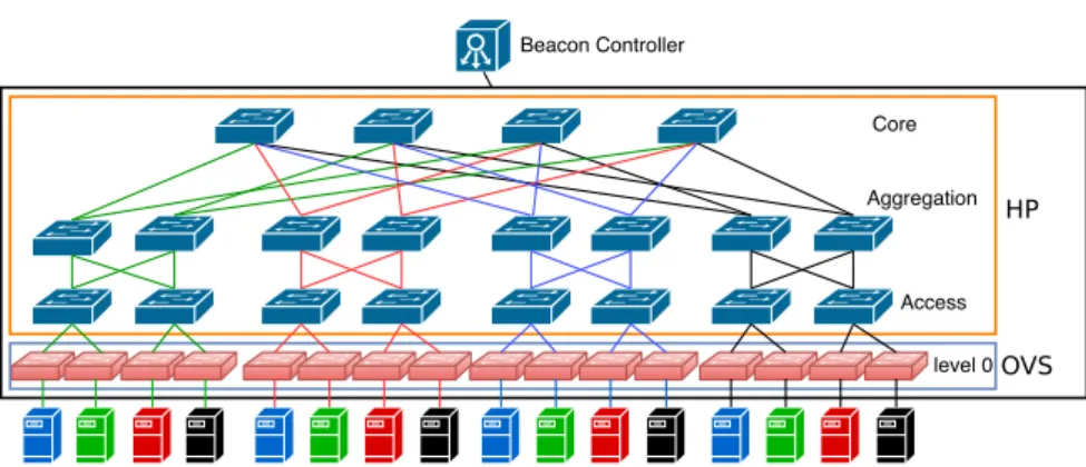
In this section, we demonstrate the effectiveness of MINNIE using an SDN testbed. The characteristics of our experimental network is described in Subsection 5.1. More specifically, we explain how with a single hardware switch and OVS switches we deploy a full k=4 Fat-Tree topology with enough clients to exceed the routing table size of the hardware switch, as well as the traffic pattern that fits the needs of our cases of study. A few details about the implementation of MINNIEwithin a Beacon controller is also provided. The obtained results are shown in Section 5.2, where we discuss the impact of MINNIEover the traffic delay, loss rate and the impact of using software rather than hardware rules. A table of content of the results obtained through simulations and experiments is available in Table 1.
5.1. Experiment settings 5.1.1. TestBed description
Our testbed consists of an HP 5400zl SDN capable switch with 4 modules, each with 24 GigaEthernet ports, and 4 DELL servers. Each server has 6 quad-core processors, 32 GB of RAM and 12 GigaEthernet ports. On each server, we deployed 4 virtual machines (VMs) with 8 network interfaces each. Each VM is connected to a dedicated Open vSwitch (OVS) switch. Each OVS switch is further connected using one physical port (of the server’s 12 ports) to the HP switch.
3Beware to distinguish the number of flows in the network from the number of rules. Here the number of rules per router is always below 1000
while the number of flows can be way higher.
(a) BCube(32, 1)
first compression
second compression
(b) k= 12 Fat-Tree
Figure 6: Scatter plot of the time to compress a table as a function of the number of flows passing through the forwarding device.
The topology of our data center network is a full k=4 Fat-Tree topology (see Figure 7), which consists of 20 SDN hardware switches. To emulate those 20 SDN hardware switches, we configured 20 VLANs on the physical switch (referred to as Vswitches). Since each VLAN possesses an independent OpenFlow instance, each VLAN behaves as an independent SDN-based switch with its proper isolated set of ports and MAC addresses. The VLAN configuration and the consequently port isolation prevents the physical switch from routing traffic among VLANs through the backplane. The Vswitches are then interconnected on the HP switch using Ethernet cables.
Each access switch (Figure 7) interconnects a single IP subnet with 16 clients, the latter emulated by two VMs, featuring up to 8 Ethernet ports each one. We detail in Section 5.1.3 the reason for choosing 16 clients per subnet.
The HP SDN switch can support a maximum of 65 536 (software + hardware) rules to be shared among the 20 emulated SDN switches. Software rules are handled in the RAM and processed by the general-purpose CPU (slow path) while hardware rules are stored in the TCAM (fast path) of the switch. The number of hardware rules that can be stored per module in our switch being equal to 750, the total switch capacity is equal to 3000 hardware rules maximum. Those 65 536 (software + hardware) available entries are not equally distributed among the 20 switches as the concept of first flow arrived-first served policy is used where the SDN rules are going to be installed on the HP switch in the order of arrival.
In one of the physical servers, we also deployed an additional VM hosting a Beacon [26] controller to manage all the switches (HP Vswitches or OVS switches) in the data center. According to [27], Beacon features high performance in terms of throughput and ensures a high level of reliability and security. To prevent the controller from becoming the bottleneck during our experiments, we configured it with 15 vCPUs (i.e., 15 cores) and 16 GB of RAM.
In the next section, we justify our choice of 16 clients per access (level 1) switch and why we have decided to add virtual OVS switches between clients and level 1 switches.
5.1.2. The need of level-0 OVS
OVS switches are used to make the controller aware of every new flow arriving in the fabric. Their routing tables are never compressed.
Without those switches, compressing at access switches with MINNIE may lead to possibly wrong routes. This phenomenon can be explained by considering the case where clients would be directly connected to access switches and MINNIEwould be used at those switches. Suppose that a correct routing imposes at one of the access switches that to reach destinations d1and d2, packets must be forwarded to port p1 while for destination d3, they should flow through port p3. Without compression, we have three rules. Now suppose that MINNIEimposes compression when the rules for destination d1 and d2 are present but the one for d3 has not been installed yet. This leads to entries (s1, d1, p1) and (s1, d2, p1) being replaced by (s1, ∗, p1). When packets from s1to d3 are sent later, they will match
Core Aggregation Access level 0 Beacon Controller HP OVS
Figure 7: Our k=4 Fat-Tree architecture with 16 OVS switches, 8 level 1, 8 level 2, and 4 level 3 switches.
the compressed forwarding rule and will reach d3using a longer path (or no path at all), as they will be forwarded to port p1and not p3. In order to avoid this behavior, the controller should be contacted for every new flow to take the best routing decision for this flow. This is the role of the OpenFlow enabled OVS switches that we introduced. They enable the controller to perform compression with an exact knowledge of the set of active flows. The net result of using those OVS switches is to enable us to perform compression starting from the access switches, giving us more opportunity to use hardware rules at these switches. In the short version of this paper [8], we did not use level-0 OVS switches, and dealt with this problem by not compressing at access switches, leading to lower compression ratios, and overloading of these switches.
Here, one could think that we just migrated the problem from the edge devices to the physical server. We believe however that this architecture represents an important step towards the solution of limited TCAM space because of the following reasons:
1. While for physical SDN-capable devices, the TCAM size is a real problem, placing one OVS switch per server, even without compressing the flow table, should not introduce major performance problems. Indeed the number of rules to be processed by each OVS switch should remain modest4while an OVS switch can handle 1000 rules at the kernel space, and up to a maximum of 200,000 rules [29].
2. Virtualization is a common service in modern data centers. Hence, virtual switches are routinely used to provide network access to the virtual machines. OpenVSwitch is natively supported by Xen 4.3 and newer releases. VMware offers support to OpenVSwitch through the NSX service for Multi-Hypervisor, which is the natural choice for large data centers. KVM, due to its native integration in Linux environments, can easily be deployed using OVS switches.
5.1.3. Number of clients chosen for the experimentations
In our Fat-Tree architecture, we can easily deduce the number of rules corresponding to a valid routing assuming that each VM talks to all other VMs not in its IP subnet. Considering no compression at all, one rule is needed for every flow passing through each switch along the path from a source to a destination. The set of flows that a switch “sees” depends on its level in the Fat-Tree. Note that here, a flow is identified by the couple IP source and IP destination addresses. Hence, for every pair of nodes A and B there are two unidirectional flows: A → B and B → A, i.e. two rules per switch on the path from A to B.
For any flow between two servers, the path goes first through the access switches to which the servers are con-nected. Assuming n servers per access switch (n= 2 in Figure 7), then each of the n servers connected to an access switch communicates with the other 7 × n servers in other subnets via outgoing and incoming flows. Overall, this represents 14n2flows going through any access switch.
4As reported in [28], a typical rack of 40 servers generate around 1300 flows per second. Therefore, each server is generating on average around
32.5 flows per second. Assuming a worst case where every per flow rule is unique and that the expiration interval for unused rules is the default value of 10 seconds of inactivity, then, an OVS switch in a single server will need to store 325 forwarding rules roughly (plus the default route to reach the local VM). This value is pretty small as compared to the 1000 rules in the fast path of an OVS switch.
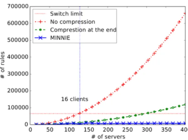
Figure 8: Total number of rules installed as a function of the number of servers, in a k= 4 Fat-Tree configuration.
Using the same argument to find the number of flows for switches at the higher levels, we have a total of 13n2 flows at each aggregation switch and 12n2 flows for a core switch. In total, 264n2 rules are needed for the entire network.
In Figure 8, we compare the total number of rules with no compression at all, and with compression (obtained via simulation) on all switches. Without compression, only 15 clients per subnet can be deployed without running out of space in the forwarding table of our entire data center (65536 entries), while up to 36 clients can be deployed with the compression at the end. Therefore, Figure 8 explains our choice of installing 16 clients per subnet. Indeed, it is the first value for which the number of rules exceeds our total limit of number of rules (67584 rules) when no compression is achieved.
5.1.4. Experimental scenarios
We aim at assessing the performance of MINNIEwith a high number of rules and with a high load. Those two objectives are contradictory in our testbed. Indeed, stressing the SDN switch in terms of rules, i.e., getting close to the limit of 65536 entries, imposes to have software rules. As software rules are handled, by definition, by the general purpose CPU of the switch (the so-called slow path), a safety mechanism has been implemented by HP to limit the processing speed to only 10 000 packets/s per VLAN. Assuming an MTU of 1500 bytes, we could not go beyond 120 Mb/s, shared between all ports in a VLAN. This is why we designed a second scenario where only hardware rules are used. In this scenario, we can fully use the 1 Gb/s link but we are limited to the 3000 hardware rules that have to be shared among the 20 switches. We thus built two scenarios to assess the performance and the feasibility of deploying MINNIEin real networks:
• Scenario 1: Low load with (large number of) software rules (LLS). This scenario enables to test the behavior of the switch when the flow table is full.
• Scenario 2: High load with (small number of) hardware rules (HLS). This scenario enables us to demonstrate that the impact of MINNIEremains negligible even when the switch transfers a load close to the line rate. For each scenario, we consider three compression cases, which are similar to the simulation scenarios presented in Section 4.1.1:
• Case 1: No compression. We fill up the routing tables of the switches and we never compress them. This test provides the baseline against which we compare results obtained with MINNIE.
• Case 2: Compression at the end (after installing the whole set of forwarding rules or when the forwarding table is full). This scenario illustrates the worst case and provides insights about the maximum stress introduced by MINNIEin the network. Indeed, in this case, we have the highest number of rules to be removed and installed after the compression executed by MINNIEwhich should be done as fast as possible.
• Case 3: MINNIE(Dynamic compression at a fixed threshold). We set a threshold to the table size and compress whenever we reach this value. We extend the third scenario of the simulations by considering three thresholds values for LLS , namely 500, 1000 and 2000 entries, and also three values for HLS: 15, 20 and 30 entries. While LLS allows to test the scalability of MINNIE in terms of number of rules in real SDN equipments, this scenario might introduce, by default, an important jitter in the network because of the usage of the general-purpose CPU to process the traffic. HLS helps to better understand the impact of the compression and forwarding table replacement over the traffic. Since the traffic rate fills up to 75% of the access links, which is not enough to introduce congestion, and packets are processed by the ASIC, we expect to have a low jitter. Hence, any sudden increase of this last will immediately suggest an important impact of the compression mechanisms over the network stability. 5.1.5. Traffic pattern
We detail in this section how the two scenarios introduced in the previous section are actually implemented in our testbed.
Low Load with software rules Scenario - LLS
In this scenario, the traffic is generated as follows: each client pings all other clients in every other subnet. This means that for each access switch, each of the 16 clients pings 112 other clients. There are no pings between hosts in the same subnet as we focus on the compression of classical IP-centric forwarding rules, which is used to route packets between different subnets, and not MAC-centric forwarding rules, as in legacy L2 switches.
We start with an initial client transmitting 5 ping packets to one other client. This train of 5 ICMP requests forms a single flow from the SDN viewpoint. We wait for this ping to terminate before sending 5 other different ping packets to another client, and so on, until all the 112 clients are pinged. When the first client finishes its pings series, a second client (hosted in the same VM) starts the same ping operation. Hence, the traffic is generated during all the experiment in a round-robin manner, among the 8 clients of each VM. Moreover, VMs do not start injecting traffic at the same time. We impose an inter-arrival period of 10 minutes between them. Hence, VM 1 starts sending traffic at time zero, while VM 2 starts at minute 10, VM 3 at minute 20, and so on. This smooth arrival of traffic in the testbed is motivated by the fact that we do not wish to overload the physical switch with OpenFlow events. Indeed, as stated in [30], commercial OpenFlow switches can handle up to 200 events/s. Since in our testbed we have 20 switches, each one handling its own flow mod (message for sending rules), packet out (message with packet to be sent) and other events, the critical number of events can be easily reached.
The experiment of this scenario ran for almost 3.5 hours. All the rules are installed in the first 2 hours and 45 minutes.
High Load with hardware rules Scenario - HLS
In this scenario, we used 1 client per VM so that the total number of rules installed (1056 total rules) is less than the hardware limit (3000 rules). Each VM starts a 50 Mbps ICMP traffic with the other clients in a round robin manner. After starting the first client machine, we wait for 75s and then start the outgoing connections for the second VM and so on, until all the machines establish connections with one other client. In this scenario, we have chosen 50 Mbps per connection in order to have a maximum of 800 Mbps load on a 1 Gbps link when all connections are established. Each experiment of this scenario ran for 1 hour and all the rules are installed in the first 20 min. As mentioned earlier, all the rules were installed in hardware in order to reach high loads.
5.1.6. MINNIEin SDN controller
When the controller compresses a table, the MINNIE SDN application5 will first execute the routing phase and then the compression phase. Hence, in a dynamic setting, when a new flow must be routed with a new entry in the router, and when the threshold of X rule will be reached, the Xthentry is first pushed to the switch (to allow the new flow to travel to the destination), and right after that, the compression is executed. Once the compression module is launched at the controller, a single OpenFlow command is used to remove the entire routing table from the switch. Then the new routes are sent immediately to limit the downtime period, that we define as the period between the removal of all old rules and the installation of all new compressed rules. When two or more switches need to be compressed at the same time, the compression is executed sequentially.
5Available at: https://sites.google.com/site/nextgenerationsdndatacenters/our-project/minnie 21