Coupled carbon-water exchange of the Amazon rain forest, II. Comparison of predicted and observed seasonal exchange of energy, CO₂, isoprene and ozone at a remote site in Rondônia

HAL Id: hal-00297742

https://hal.archives-ouvertes.fr/hal-00297742

HAL is a multi-disciplinary open access

archive for the deposit and dissemination of sci-entific research documents, whether they are pub-lished or not. The documents may come from teaching and research institutions in France or abroad, or from public or private research centers.

L’archive ouverte pluridisciplinaire HAL, est destinée au dépôt et à la diffusion de documents scientifiques de niveau recherche, publiés ou non, émanant des établissements d’enseignement et de recherche français ou étrangers, des laboratoires publics ou privés.

Coupled carbon-water exchange of the Amazon rain

forest, II. Comparison of predicted and observed

seasonal exchange of energy, CO2, isoprene and ozone at

a remote site in Rondônia

E. Simon, F. X. Meixner, U. Rummel, L. Ganzeveld, C. Ammann, J.

Kesselmeier

To cite this version:

E. Simon, F. X. Meixner, U. Rummel, L. Ganzeveld, C. Ammann, et al.. Coupled carbon-water exchange of the Amazon rain forest, II. Comparison of predicted and observed seasonal exchange of energy, CO2, isoprene and ozone at a remote site in Rondônia. Biogeosciences Discussions, European Geosciences Union, 2005, 2 (2), pp.399-449. �hal-00297742�

BGD

E. Simon et al. Title Page Abstract Introduction Conclusions References Tables Figures J I J I Back Close

Full Screen / Esc

Print Version Interactive Discussion

Biogeosciences Discussions, 2, 399–449, 2005 www.biogeosciences.net/bgd/2/399/

SRef-ID: 1810-6285/bgd/2005-2-399 European Geosciences Union

Biogeosciences Discussions

Biogeosciences Discussions is the access reviewed discussion forum of Biogeosciences

Coupled carbon-water exchange of the

Amazon rain forest, II. Comparison of

predicted and observed seasonal

exchange of energy, CO

₂

, isoprene and

ozone at a remote site in Rond ˆ

onia

E. Simon1, F. X. Meixner1, U. Rummel2, L. Ganzeveld3, C. Ammann4, and J. Kesselmeier1

1

Biogeochemistry Dept., Max Planck Institute for Chemistry, Mainz, Germany

2

Meteorologisches Observatorium Lindenberg, Deutscher Wetterdienst, Germany

3

Atmospheric Chemistry Dept., Max Planck Institute for Chemistry, Mainz, Germany

4

Swiss Federal Research Station for Agroecology and Agriculture, Z ¨urich, Switzerland Received: 24 February 2005 – Accepted: 14 March 2005 – Published: 7 April 2005 Correspondence to: E. Simon (simon@mpch-mainz.mpg.de)

BGD

E. Simon et al. Title Page Abstract Introduction Conclusions References Tables Figures J I J I Back Close

Full Screen / Esc

Print Version Interactive Discussion Abstract

A one-dimensional multi-layer scheme describing the coupled exchange of energy and CO₂, the emission of isoprene and the dry deposition of ozone is applied to a rain forest canopy in southwest Amazonia. The model was constrained using mean diel cycles of micrometeorological quantities observed during two periods in the wet and dry season 5

1999. Predicted net fluxes and concentration profiles for both seasonal periods are compared to observations made at two nearby towers.

The predicted day- and nighttime thermal stratification of the canopy layer is con-sistent with observations in dense canopies. The observed and calculated net fluxes above and H₂O and CO₂concentration profiles within the canopy show a good agree-10

ment. The predicted net carbon sink decreases from 2.5 t C ha−1yr−1 for wet sea-son conditions to 1 t C ha−1yr−1for dry season conditions, whereas observed and pre-dicted midday Bowen ratio increases from 0.5 to 0.8. The evaluation results confirmed a seasonal variability of leaf physiological parameters, as already suggested in the companion study. The predicted midday canopy net flux of isoprene increased from 15

7.1 mg C m−2h−1 during the wet season to 11.4 mg C m−2h−1 during the late dry sea-son. Applying a constant emission capacity in all canopy layers, resulted in a disagree-ment between observed and simulated profiles of isoprene concentrations, suggesting a smaller emission capacity of shade adapted leaves and deposition to the soil or leaf surfaces. Assuming a strong light acclimation of emission capacity, equivalent to a 66% 20

reduction of the standard emission factor for leaves in the lower canopy, resulted in a better agreement of observed and calculated concentration profiles and a 30% reduc-tion of the canopy net flux. The mean calculated ozone flux for dry season condireduc-tion at noontime was ≈12 nmol m−2s−1, agreeing well with observed values. The correspond-ing deposition velocity increased from 0.8 cm s−1 to >1.6 cm s−1 in the wet season, 25

which can not be explained by increased stomatal uptake. Considering reasonable physiological changes in stomatal regulation, the predicted value was not larger than 1.05 cm s−1. Instead, the observed fluxes could be explained with the model by

BGD

E. Simon et al. Title Page Abstract Introduction Conclusions References Tables Figures J I J I Back Close

Full Screen / Esc

Print Version Interactive Discussion

creasing the cuticular resistance to ozone deposition from 5000 to 1000 s m−1. For dou-bled atmospheric CO₂concentrations the model predicts a strong increase of surface temperatures (0.1–1◦C) and net assimilation (22%), a considerable shift in the energy budget (≈25% decreasing transpiration and increasing sensible heat), a slight increase of isoprene emissions (10%) and a strong decrease of ozone deposition (35%). 5

1. Introduction

Within the last decade, detailed biosphere-atmosphere models have been developed to describe the exchange of energy and important atmospheric trace gases like CO₂, ozone and isoprene between the terrestrial vegetation and the lower atmosphere (

Sell-ers et al., 1992; Leuning et al.,1995;Baldocchi and Meyers, 1998; Baldocchi et al., 10

1999). These models integrate knowledge from different scientific disciplines and may serve as helpful tools in geophysical research: in prognostic applications, they can be used to study the feedback between atmospheric and biophysical processes (such as the effect of CO₂ fertilization) and diagnostically, they can be used as a substitution and completion of costly field measurements.

15

In a companion paper, Simon et al.(2005a) describe a one-dimensional multilayer canopy model of coupled carbon-water exchange. This scheme includes detailed de-scriptions of ecophysiological exchange processes at the leaf scale, which are con-nected to the canopy scale by a Lagrangian dispersion model of vertical turbulent transport. Commonly this model type is referred to as the “CANVEG” scheme, origi-20

nally invented byBaldocchi(1992) andBaldocchi and Meyers(1998). We adapted the CANVEG scheme for application to the Amazon rain forest. Using informations and data pools from intensive field campaigns, a generic characterization and parameteri-zation of biophysical properties of the predominant vegetation type within the Amazon basin is given. In summary, the results presented in the companion paper include a 25

characterization of mean canopy structure, the distribution of photosynthetic capac-ity and a normalized profile of horizonal wind speed. The subroutines to calculate

BGD

E. Simon et al. Title Page Abstract Introduction Conclusions References Tables Figures J I J I Back Close

Full Screen / Esc

Print Version Interactive Discussion

the canopy radiation field and soil surface exchange as well as leaf photosynthesis and stomatal conductance, considering wet and dry season conditions, are evaluated using scale appropriate data. Finally, the sensitivity of predicted net fluxes to key parameter uncertainty is investigated and the uncertainty range of leaf physiological parameters is derived. The parameterization of the Lagrangian dispersion sub-model is discussed 5

and evaluated in detail in a further study (Simon et al., 2005b1, hereafter referred to as S2005b).

In the present study, the parameterized model is applied to a remote site in Rond ˆonia, Sout-West Brazil. Calculated net fluxes and vertical scalar profiles of H₂O, CO₂, iso-prene and ozone are compared to measurements made at two nearby micrometeoro-10

logical towers during the late wet and late dry season 1999. The model is constrained using observed surface-layer meteorology and soil moisture status and soil tempera-ture measured just below the soil surface. The following questions are addressed:

1. Concept validation: Are the environmental boundary-conditions in steady-state or does the coupling of surface exchange and vertical dispersion result in numerical 15

instabilities of the predicted canopy temperature and H₂O and CO₂ concentra-tions?

2. Model evaluation: Is the model predicted thermal stratification of the canopy con-sistent with observations? How well does the model predicted fluxes and concen-tration profiles of CO₂, H₂O, isoprene and O₃agree with observations?

20

3. Diagnostic model application: To what extend does the model explain the ob-served variabilities of net fluxes and concentration profiles and how does the model contribute to our understanding of the processes which are involved in the exchange of important atmospheric trace gases?

1

Simon, E., Lehmann, B., Ammann, C., Ganzeveld, L., Rummel, U., Nobre, A., Araujo, A., Meixner, F., and Kesselmeier, J.: On Lagrangian dispersion of 222Rn, H2O, and CO2 within the Amazon rain forest, Agric. For. Meteorol., submitted, 2005b.

BGD

E. Simon et al. Title Page Abstract Introduction Conclusions References Tables Figures J I J I Back Close

Full Screen / Esc

Print Version Interactive Discussion

Topic (1) is related to basic model assumptions. It has to be shown, that the inter-active coupling of surface exchange and vertical mixing does not result in unstable or unrealistic numerical solutions, due to unsteady environmental conditions. This might occur if for example the air temperature or CO₂concentration of a single canopy layer increases with every iteration step of surface exchange because the calculated vertical 5

mixing rate is too slow. Topic (2) includes mainly a comparison of model results and observations. Measurements of leaf temperature and temperatures of the surrounding canopy air have not been available for direct evaluation. However, the calculated ther-mal stratification of the canopy may serve as a good indicator of model consistency. In the real world, the lower part of dense canopies shows often a typical diel pattern, 10

which is the reverse compared to the atmospheric boundary-layer above (Jacobs et al.,

1994; Bosveld et al.,1999, specifically for Amazon rain forest see Kruijt et al.,2000; S2005b). For further validation, direct eddy covariance fluxes of sensible heat, latent heat, CO₂ and O₃ measured above the canopy are used. Furthermore, the reliability of model results is advanced by including a comparison of measured and calculated 15

scalar profiles of CO₂, H₂O, isoprene and O₃. This is very meaningful because the pre-dicted fluxes may be in agreement with the measurements while the prepre-dicted concen-trations profiles are not very realistic (as an example seeBaldocchi,1992). By using different data sets for model parameterization, application and evaluation (e.g. enclo-sure meaenclo-surements at the leaf level in the companion paper, in-canopy concentration 20

profiles and canopy net fluxes at the canopy level in the present study) a profound and complementary evaluation of our current knowledge on canopy processes is per-formed. (3) In general, the variability of energy and trace gas exchange is imposed by short- and longterm frequencies, i.e. the diel and annual solar cycles, respectively. We assessed the diel variabilities by analyzing mean diel cycles of net fluxes and typical 25

day- and nighttime vertical concentration profiles. The longterm variability is charac-terized mainly by periods of high and low rainfall, which may trigger ecophysiological (stomatal conductance, photosynthesis) or structural (LAI) acclimations of the rain for-est (Malhi et al.,1998; Williams et al., 1998; Andreae et al., 2002). This question is

BGD

E. Simon et al. Title Page Abstract Introduction Conclusions References Tables Figures J I J I Back Close

Full Screen / Esc

Print Version Interactive Discussion

assessed by combining key model parameter uncertainties inferred in the companion paper (Simon et al., 2005a) with a seasonal comparison of the observed and calcu-lated mean diel cycles of canopy net fluxes. Furthermore, current isoprene emission and ozone deposition algorithms have been integrated into the model and the predicted fluxes and scalar profiles of these tracers are evaluated and discussed as well. Finally, 5

we applied a future climate scenario, which assumes doubled atmospheric CO₂ con-centrations. The resulting canopy net fluxes and surface temperatures are compared to the predictions for present climate conditions.

2. Materials and methods

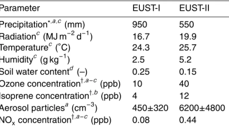
2.1. Site description and field data 10

The modified CANVEG scheme is applied to a primary tropical rain forest in Rond ˆonia (Reserva Jaru, seeSimon et al.,2005a). This site was the main forest research site of LBA-EUSTACH2and is described in detail byAndreae et al.(2002). Measurements have been performed simultaneously at two towers, RBJ-A and RBJ-B, during two intensive field campaigns, hereafter referred to as EUST-I and EUST-II, respectively, 15

coinciding with the late wet (April–May) and late dry season (September–October) in 1999. At RBJ-B, eddy covariance fluxes of CO₂, H₂O, and sensible heat were mea-sured at 62 m above the ground, whereas concentration profiles of CO₂and H₂O were sampled at 62.7, 45, 35, 25, 2.7 and 0.05 m (Andreae et al., 2002). At RBJ-A, eddy covariance fluxes of CO₂, H₂O, sensible heat and ozone were measured at 53 m above 20

the ground, whereas concentrations profiles of CO₂, H₂O, and ozone were sampled at 51.7, 42.2, 31.3, 20.5, 11.3, 4, 1 and 0.3 m (Rummel,2005;Andreae et al.,2002). The input data to constrain the model (surface-layer meteorology above the canopy i.e. rel-ative humidity, air temperature, barometric pressure, incoming global radiation, mean

2

Large-scale Biosphere-atmosphere experiment in Amazonia – EUropean Studies on trace gases and Atmospheric CHemistry

BGD

E. Simon et al. Title Page Abstract Introduction Conclusions References Tables Figures J I J I Back Close

Full Screen / Esc

Print Version Interactive Discussion

horizontal wind speed, standard deviation of vertical wind speed, background ozone concentration; soil moisture status and temperature at −0.05 m) has been measured at RBJ-A. Additionally, measurements of isoprene concentrations were made simulta-neously at 1, 25, 45 and 52 m height during a short period at the end of the dry season, as described in detail byKesselmeier et al.(2002). Most of the data have been pub-5

lished recently (a comprehensive overview is given byAndreae et al.,2002). The time series of the micrometeorological data, net fluxes and scalar profiles (except isoprene), available with a time resolution of 30 min, have been averaged to hourly means of two diel cycles for wet (EUST-I) and dry season (EUST-II) conditions, respectively. Note that the time given in all graphs indicates interval start (e.g. 8 h represents the time 10

interval from 8–9 h).

The net fluxes of sensible heat, H₂O, CO₂, and ozone measured above the canopy have to be corrected by the canopy volume storage flux for a direct comparison with the model predicted “instantaneous” fluxes. The storage fluxes for CO₂and ozone are calculated according toGrace et al.(1995) from the temporal evolution of the diurnally 15

averaged vertical concentration profiles. The empirical relationship ofMoore and Fisch

(1986), evaluated for RBJ-A byRummel(2005), was applied to determine the energy storage terms, using the temperature and humidity observed above the canopy. 2.2. Meteorological overview

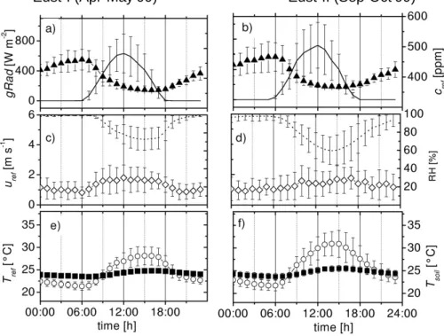
The mean diel cycles of micrometeorological forcing parameters observed at RBJ-A 20

during EUST-I and EUST-II are shown in Fig.1. A seasonal comparison of additional climatic variables is listed in Table 1. Global radiation reaches maximum values of 400–900 W m−2around noon time with distinctly larger values during the late dry sea-son. The CO₂concentration shows a strong diurnal variability with maximum and min-imum values between 460 and 365 ppm during night- (4–6 h) and daytime (15–16 h), 25

respectively. The wet season daytime minimum values are slightly lower (361 ppm) compared to the dry season (367 ppm). Furthermore, relative humidity during EUST-I was larger and incoming radiation and temperature were lower compared to the dry

BGD

E. Simon et al. Title Page Abstract Introduction Conclusions References Tables Figures J I J I Back Close

Full Screen / Esc

Print Version Interactive Discussion

season. Mean daytime maximum temperature and diurnal amplitude was 3◦C higher during the dry season, coinciding with a decrease of relative humidity. The noon time values decreased from 72% to 60%, whereas the specific humidity was twice as high for dry compared to wet season conditions, respectively. The soil temperature was only slightly higher during the dry season whereas the mean soil water content decreased 5

approximately from 25 to 15%. The wet-to-dry seasonal changes of humidity, tem-perature, and radiation were accompanied by the occurrence of large-scale biomass burning leading to a strong increase in aerosol particles and ozone concentrations (see Table1). In contrast, the mean diel cycles of horizontal wind speed (Fig. 1c, d) and other turbulent quantities are very similar for both seasonal periods.

10

2.3. Model setup

The parameterization of the CANVEG scheme and the Lagrangian transport sub-model are described in detail inSimon et al. (2005a) and S2005b, respectively. A bi-modal leaf area density distribution with LAI=6 and a mean canopy height h_c=40 m is ap-plied. A number of 8 equidistant canopy layers of 5 m depth has been selected with a 15

surface layer of 13 m depth above h_c and below z_ref=53 m. Predicted canopy albedo is optimized by scaling leaf optical parameters. Soil respiration is calculated applying the observed reference value of 3.3 µmol m−2s−1 at 25◦C and an activation energy of 60 kJ mol−1. The light acclimation parameter for leaf photosynthesis is set to k_N=0.2 with a maximum carboxylation rate of 50 µmol m−2s−1 at the canopy top. The temper-20

ature dependence of leaf photosynthesis is calculated using optimized values for the activation energy of electron transport and entropy (H_{v J}=108 and S_J=0.66 kJ mol−1, respectively). For details seeSimon et al.(2005a).

The question whether the observed seasonal variability of canopy net fluxes may be driven by changing leaf physiology (see Sect.1,Andreae et al.,2002) is addressed by 25

modifying three leaf model parameters within their inferred uncertainty range (see Ta-ble2): A reference parameterization using the same values for both seasonal periods (1), a parameterization predicting higher stomatal conductance rates (g_s) for EUST-I

BGD

E. Simon et al. Title Page Abstract Introduction Conclusions References Tables Figures J I J I Back Close

Full Screen / Esc

Print Version Interactive Discussion

by increasing the parameter correlating g_s with net assimilation A_n (2, see also Lloyd

et al.,1995a), and a third parameterization predicting lower A_nfor EUST-II by decreas-ing the quantum yield of electron transport (α, the light-use efficiency and initial slope of light response) and the shape parameter of the hyperbolic light response function (θ).

5

Isoprene emission at the leaf scale is calculated according to Guenther et al.

(1993). A standard emission factor of 24 µg C g−1h−1 and a specific leaf dry weight of 125 g m−2 (Guenther et al.,1995) is used for all leaves. These numbers are equiva-lent to an assumed fraction of 30% isoprene emitting species, each having a standard emission factor of 80 µg C g−1h−1(see alsoHarley et al.,2004). Ozone uptake is cal-10

culated by applying the concept of dry deposition, assuming that chemical sources and sinks for ozone production and consumption within the canopy are neglected. Gener-ally, the dry deposition velocity

v_{d ,x} = Fx

c_x(z_ref). (1)

then represents the kinematic flux F_xof a tracer x, normalized by the tracer concentra-15

tion at z_ref above the canopy. Eq. (1) is applicable for trace gases which are deposited to leaf and soil surfaces, whereby the trace gas concentration inside the leaf (and soil) is assumed to be zero (see alsoBaldocchi et al.,1987;Ganzeveld and Lelieveld,1995). In a multilayer scheme, v_{d ,x} is given by the parallel uptake in all canopy layers ac-cording to

20

v_{d ,x} = v_{d ,soi l} +Xm

i=0vd ,i (2)

where v_{d ,i} represents the deposition to the leaf surface Λ_i in layer i . v_{d ,i} and soil deposition (v_{d ,soi l}) are calculated according to

v_{d ,i} Λi = 1 r_a(z_i)+ r_{l eaf ,O} 3 (3)

BGD

E. Simon et al. Title Page Abstract Introduction Conclusions References Tables Figures J I J I Back Close

Full Screen / Esc

Print Version Interactive Discussion v_{d ,soi l} = 1 r_a(z= 0) + r_{soi l ,O} 3 . (4)

The aerodynamic resistance to turbulent transport from z_ref to z_i is equivalent to the integrated dispersion coefficient between these heights. According toBaldocchi et al.

(1987), the total leaf resistance to ozone uptake (r_{l eaf ,O}

3) for hypo-stomatous leaves can be divided into a stomatal and cuticular pathway according to

5 1 r_{l eaf ,O} 3 = 1 r_b,O 3+ rs,O3+ rm,O3 + 2 r_b,O 3+ rcut,O3 . (5)

The leaf boundary-layer (r_b) and stomatal (r_s) resistance are derived from the con-ductances for water vapor using the ratio’s of molecular diffusivities (Massman,1998). The factor of two on the right side of Eq. (5) indicates, that cuticular exchange occurs at both leaf sides. The intercellular ozone concentration and consequently the mes-10

ophyll resistance are assumed to be zero (Chameides, 1989; Weseley, 1989;

Neu-bert et al.,1993;Gut et al.,2002a). Although the cuticular resistance (r_cut,O

3) is rel-atively large (Gut et al., 2002a), the significance of this pathway to total deposition has been shown recently byRummel(2005), estimating a value of 4000–5000 s m−1. The resistance to soil deposition was estimated as 188 s m−1 from dynamic chamber 15

measurements byGut et al. (2002a). Adding this value to the bulk soil surface resis-tance (transport from the mean height of the lowest canopy layer at 2.5 m to the soil surface 1/g_{soi l}≈500 s m−1, see companion paper) results in a total soil resistance of

r_{soi l ,O}

3≈700 s m

−1

.

The application of the dry deposition concept for ozone within the framework of a 20

multilayer model is not straightforward because chemical reactions with ozone may become important. Meixner et al. (2002) recently compared the chemical, biologi-cal and transport timesbiologi-cales of relevant reactions of the NO-NO₂-O₃ triad (Bakwin

et al.,1990;Jacob and Wofsy,1990;Chameides and Lodge,1992;Yienger and Levy,

1995;Ganzeveld et al.,2002). Above the canopy, chemical reactions are much slower 25

compared to turbulent exchange and can be neglected. At 11 m in the lower canopy, 408

BGD

E. Simon et al. Title Page Abstract Introduction Conclusions References Tables Figures J I J I Back Close

Full Screen / Esc

Print Version Interactive Discussion

turbulent transport is still efficient, and the biological uptake of ozone is one order of magnitude faster than ozone chemistry. Below 10 m, the photolysis rate is too small for ozone production by NO₂ oxidation, so that only ozone destruction by NO has to be considered. In this case, the chemical, biological and transport timescales are on the same order of magnitude. However, this is only relevant for the NO budget: The 5

maximum chemical loss term of ozone due to reduction by NO is equivalent to the total soil NO flux, which is at least one order of magnitude lower (<0.7 nmol m−2s−1) than the mean observed ozone fluxes (>3 nmol m−2s−1Gut et al.,2002b;Rummel,2005).

3. Results and discussion

3.1. Canopy thermal stratification 10

The assumption of steady-state environmental conditions implies that leaf surface ex-change and vertical mixing are in balance. This assumption is usually fulfilled when meteorological quantities change slowly. However, for short periods the environmental conditions may change rapidly, e.g. due to rainfall or large scale turbulence structures. Therefore, only time-averaged micrometeorological quantities were considered and pe-15

riods with rain were rejected. The day- and nighttime transition periods at sunrise and sunset represent further situations, where micrometeorological conditions are un-steady. Probably the most appropriate indicators for conditions where the steady-state assumption is not fulfilled are the temperature differences between the surface and the ambient air within and above the canopy (T_s−T_a, T_a−T_ref, respectively). Therefore, the 20

predicted canopy thermal stratification has been analyzed in detail.

Figure2shows the diel cycle of the calculated differences between the mean foliage temperature, the ambient air within and the surface layer above the canopy (for EUST-I) and the number of model iterations required for model conversion (I and EUST-II). The mean foliage and ambient air temperatures (T_s,av, T_a,av) are calculated as the 25

BGD

E. Simon et al. Title Page Abstract Introduction Conclusions References Tables Figures J I J I Back Close

Full Screen / Esc

Print Version Interactive Discussion

air T_a, respectively. T_s is calculated as the sunlit and shaded leaf fraction weighted surface temperature. During daytime, the foliage and canopy air are heated by so-lar radiation and the model predicts T_s,av−T_a,av≈1.5◦C and T_a,av−T_ref≈0.5◦C at noon-time. During sunset, the foliage cools off, the radiation budget of the canopy changes its sign and steady-state calculations fail to converge. Obviously, model assumptions 5

are violated under these circumstances since the micrometeorological conditions are changing towards a new state. This highlights interesting interactions between the vegetation layer, the soil surface below and the atmospheric boundary-layer above. For nighttime conditions, model calculations are consistent again predicting negative gradients T_s,av−T_a,av≈T_a,av−T_ref≈−0.4◦C. As shown in Fig.2b, 2–10 iterations are re-10

quired for conversions for daytime conditions and there is a negative correlation with ∆T (Fig.2a). For nighttime conditions, a constant number of 4 iterations is required.

Stable model solutions for steady-state environmental conditions are shown in more detail in Fig.3. For daytime conditions, the model predicts large temperature gradients across the leaf boundary layer (T_s−T_a) and sunlit and shaded leaf surfaces. This is very 15

important for physiological processes, which imply usually a non-linear temperature response. Assuming a typical Q₁₀-value of 2, a temperature increase of 5◦C would increase the physiological response by 50%.

As observed in real canopies, foliage temperatures reaches maximum values in the upper canopy, where the highest irradiance is absorbed. At 0.75 h_c, the mean leaf 20

temperature is mostly determined by the surface temperature of sunlit leaves, which is 2–4◦C higher compared to shaded leaves. Close to the ground, T_s−T_abecomes small. To assess the sensitivity of these calculations to leaf physiological parameters, the parameter modifications listed in Table2 have been applied in additional simulations (represented as error bars shown in Fig. 3). Increasing stomatal conductance (by 25

increasing a_N) has a cooling effect on T_sresulting in a decrease of 0.3–1.2◦C for EUST-I. Decreasing photosynthesis (by decreasing α and θ) leads to decreasing stomatal conductance and results in higher leaf temperatures (0.1–0.5◦C) for EUST-II.

The thermal stratification of the canopy air space has also a strong impact on the 410

BGD

E. Simon et al. Title Page Abstract Introduction Conclusions References Tables Figures J I J I Back Close

Full Screen / Esc

Print Version Interactive Discussion

turbulence regime. The diel pattern, which has been calculated by the model, is very similar to what we expect for dense vegetations. In the early morning, the soil surface is warmer than the canopy air above. Later in the day, the foliage is being heated by solar radiation resulting in an unstable stratification of the surface layer above. Since the maximum of absorbed radiation occurs in the upper canopy, the lower canopy layer 5

remains cooler and becomes stable up to 10 m height (0.25 h_c). During the night, the stratification in the atmospheric boundary-layer is usually very stable because the surface layer is cooler than the air above (Stull,1988). However within dense canopies, the stratification is reversed, because the maximum cooling effect occurs in the upper canopy where biomass is most dense. In combination with soil heat storage, a weak 10

but efficient convective energy flux is generated in the lower canopy (seeJacobs et al.,

1994;Kruijt et al.,2000, S2005b).

3.2. Seasonal exchange of CO₂and energy

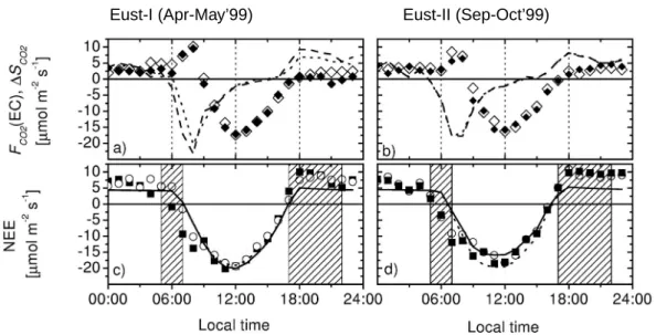
The predicted sensible heat (H) and latent heat (LE ) fluxes, net ecosystem exchange of CO₂(NEE) and vertical scalar profiles of H₂O and CO₂obtained for I and EUST-15

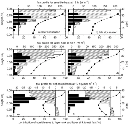
II meteorology are compared to observations at the two towers RBJ-A and RBJ-B. The diel cycles of the net fluxes are shown in Figs.4and5. The calculated midday vertical source/sink distributions, flux profiles and the relative contribution of sunlit leaves to the exchange of single canopy layers are shown in Fig.6. The eddy covariance fluxes measured above the canopy (F (EC)) have been corrected for the canopy storage∆S 20

(see Sect.2.1).

For both seasonal periods, most of the available energy at the canopy surfaces is converted into latent heat (LE ), especially later during the day. The observed and calculated diel cycles of the Bowen ratio show a strong decline from values close to one just after sunrise to values <0.3 just before sunset. In the early morning and 25

late afternoon,∆S is large, especially for CO₂, exceeding even the net flux measured above the canopy. For H and LE ,∆S contributes 40–60 W m−2. There is generally a good agreement between the RBJ-A and RBJ-B tower EC measurements and storage

BGD

E. Simon et al. Title Page Abstract Introduction Conclusions References Tables Figures J I J I Back Close

Full Screen / Esc

Print Version Interactive Discussion

fluxes. The sensible heat and CO₂ fluxes measured at RBJ-A in the afternoon and morning hours, respectively, are slightly higher compared to RBJ-B, whereas morning

LE fluxes are slightly lower (<4%). This variability may result from different tower

source areas and reflect the measurement uncertainty (for a discussion of the source area and fetch conditions at RBJ-A seeRummel,2005) .

5

Generally, a good agreement is obtained between model calculated fluxes and ob-servations, especially when seasonal physiological changes are considered. The me-teorological changes from EUST-I to EUST-II (Fig. 1) result in larger energy fluxes and Bowen ratios (i.e. increased fractions of sensible heat) and lower assimilation rates (in relation to the incoming radiation). Using the reference parameterization (see 10

Sect.2.3), the model predicts ≈20% larger sensible heat fluxes for EUST-I compared to observations (see also changes in the Bowen ratio shown in Fig. 4i–j). Increasing stomatal conductances for EUST-I, leads to a better agreement between model cal-culations and observations. For midday conditions, this goes along with a shift in the energy budget: LE increases and H decreases by 50 W m−2 compared to the model 15

calculations using the reference parameterization (Fig.6). For the calculated NEE this modification is less important since net assimilation is less sensitive to the modified stomatal parameter than H and LE (see Table2, see alsoSimon et al.,2005a).

Reducing the photosynthesis parameters for EUST-II, results in a 10–20% decrease of NEE and a better agreement between model calculations and observations. Ab-20

solute peak NEE at noon time is reduced from 19.5 to 15.8 µmol m−2s−1 (Fig. 6f). The large contribution of sunlit leaves to net assimilation of the lower canopy (>60%) highlights the non-linearity of photosynthetic light response and the significance of a two-stream canopy radiation model, which accounts for the different attenuation of dif-fusive and direct beam radiation. For sensible and latent heat this effect is less pro-25

nounced and the contribution of shaded leaves to the energy fluxes of the lower canopy is larger (40–60%). The maximum source/sink strength for sensible heat, latent heat and net assimilation is located in the upper canopy at 25–30 m with contributions of approximately 35, 33, and 43% to the canopy net flux, respectively. The location of

BGD

E. Simon et al. Title Page Abstract Introduction Conclusions References Tables Figures J I J I Back Close

Full Screen / Esc

Print Version Interactive Discussion

the maxima coincides with the maximum leaf area density several meters below the maximum of foliage temperature (Fig.3).

The nighttime energy fluxes are generally small, especially for latent heat, and the modifications of physiological parameters have no effect, because the modeled nighttime stomatal conductance and leaf CO₂ exchange depend only on minimum 5

stomatal conductance (g_s0=0.01 mol m−2s−1) and the dark respiration rate. The pre-dicted nighttime sensible heat fluxes are within a range of 10–30 W m−2 and agree well with observed values. The predicted nighttime CO₂ flux (≈4.5 µmol m−2s−1) is significantly smaller compared to the observations (NEE≈6.5, F_CO

2(E C)≈3.2, ∆SCO2≈3.3 µmol m

−2

s−1). However, it should be noted that there is a large uncer-10

tainty in nighttime EC measurements (seeGoulden et al.,1996;Mahrt,1999;Araujo

et al.,2002, S2005b). Furthermore, leaf respiration in the dark differs from light respi-ration during the day (Brooks and Farquhar,1985;Lloyd et al.,1995b), which is not yet considered in the present approach.

For a detailed analysis of the observed and calculated scalar profiles, the period 15

from 14-15 h has been selected, because the afternoon storage fluxes are relatively small (see Figs. 4, 5). A comparison of the observed and predicted CO₂ and H₂O concentration profiles is shown in Fig.7. In general, the seasonal and diurnal variabil-ities are not very large and the selected profiles represent typical patterns for daytime conditions. Since the largest emission and uptake rates for H₂O and CO₂, respectively, 20

usually coincide with the highest turbulence intensities around noon time, increased vertical gradients are counterbalanced by enhanced vertical mixing rates. Since the whole vegetation layer represents a strong H₂O source during the day, H₂O concen-trations increase with decreasing height and reach maximum values close to the soil surface where turbulent mixing is weak. As shown in Fig.7a, b, the predicted H₂O pro-25

files agree with the EUST-I and EUST-II observations and can also explain the steeper H₂O gradients near the soil surface observed during the drier period (EUST-II). A good agreement between observations and model predictions is also obtained for the day-time CO₂ concentration profiles. Consistent with observations, the predicted vertical

BGD

E. Simon et al. Title Page Abstract Introduction Conclusions References Tables Figures J I J I Back Close

Full Screen / Esc

Print Version Interactive Discussion

gradient changes its sign at ≈10 m above ground, where CO₂uptake by the vegetation balances the emission by the soil. Although soil CO₂emissions are much lower than the uptake by the vegetation, gradients (with respect to z_ref) above 10 m are smaller due to much higher ventilation rates. For both, H₂O and CO₂, the predicted vertical profile is rather insensitive to modifications of the physiological parameters for stomatal 5

conductance and photosynthesis (in contrast to the net fluxes as shown inSimon et al.,

2005a).

For nighttime conditions, the environmental conditions are most likely not in steady-state, as indicated by large storage terms, especially for CO₂(see Figs.4a, b, e, f and

5a, b). In the case of H₂O, the observed vertical gradients are close to zero and the 10

differences between the measurements made at both towers are larger as the differ-ences between calculations and observations. In the case of CO₂, the model fails to predict the observed CO₂ gradients in size and shape. The observed concentrations are much higher as model predictions. The observed gradients at the taller tower RBJ-B (z_ref=62.7 m) are, compared to RBJ-A (z_ref=53 m), on the same order of magnitude 15

larger (5–20 ppm) as the observed gradients at RBJ-A compared to model calculations (results not shown). Possible reasons for the underestimation of the nighttime CO₂ pro-files by the model have been investigated by conducting a sensitivity analysis including four parameters:

- As mentioned above, the nighttime CO₂flux is probably underestimated because 20

the approach to calculate leaf dark respiration may be not fully appropriate. There-fore, leaf respiration was increased to 200% in scenario 1.

- For the predicted soil respiration, we assume an uncertainty of 50 %, which may significantly contribute to near-surface CO₂ concentrations. Therefore soil respi-ration was increased to 150% in scenario 2.

25

- A statistical analysis of the input data showed generally a good agreement be-tween the arithmetic mean and median values for all input parameters, except for the standard deviation of vertical wind speed above the canopy (σ_wref), which

BGD

E. Simon et al. Title Page Abstract Introduction Conclusions References Tables Figures J I J I Back Close

Full Screen / Esc

Print Version Interactive Discussion

represents the main forcing parameter of turbulent mixing (Raupach, 1989, see also S2005b). As a consequence of few “untypical” nighttime cases with high turbulence, the arithmetic mean of σ_wref for nighttime conditions is 40% larger compared to its median value. Therefore, we considered a 50% lower value of

σ_wref in scenario 3. 5

- From comprehensive studies on in-canopy turbulence at the Jaru site (Kruijt et al.,

2000;Rummel,2005) it is well known, that the upper and lower canopy layer are strongly decoupled, especially during nighttime. The most frequent turbulent ed-dies induced by surface-layer friction are to weak and their length scale is to small to reach the lower canopy. This means that vertical transport across a “decou-10

pling height” within the canopy is suppressed. We estimated the potential impact of this effect on vertical scalar dispersion, by modifying the parameterization of the dispersion matrix (see S2005b), assuming 80% inflection of the profile of the standard deviation of vertical wind speed σ_w(z) at 0.5 h_c (scenario 4).

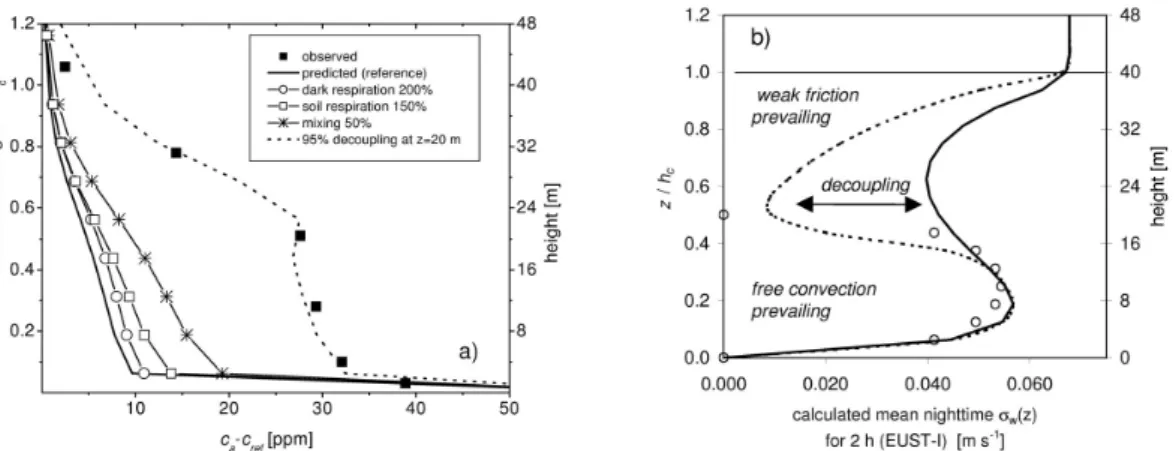
The results of the sensitivity analysis are shown in Fig.8a. Neither increased leaf, 15

nor increased soil respiration are sufficient to produce large vertical gradients within the canopy compared to the original parameterization. Whereas the effect of leaf respira-tion is generally small, increased soil respirarespira-tion affects mainly the CO₂gradients close to the ground. In contrast, the predicted profile is very sensitive to reduced turbulence which increases the gradients c_a−c_ref by almost 100%. However, this effect is not suf-20

ficient to explain the observed shape of the CO₂profile, which shows small gradients in the lower canopy and a steep decrease of CO₂ concentration above 0.5 h_c. The inflection of σ_w(z) increased the vertical dispersion coefficient (in units of a resistance) across the layer from 17.5 to 22.5 m by ≈95% (scenario 4). This strong decoupling ef-fect increased the calculated CO₂concentration in the lower canopy by a factor of two 25

and may explain, in combination with the effect of weak turbulence (median instead of average value of σ_wref), the observed profile very well.

parameteri-BGD

E. Simon et al. Title Page Abstract Introduction Conclusions References Tables Figures J I J I Back Close

Full Screen / Esc

Print Version Interactive Discussion

zation, is shown in Fig.8b. The maximum in the lower canopy results from the con-vective part of the calculations and is almost as high as σ_wref above the canopy. The modification of σ_w(z) seems not unrealistic. For the lower canopy, it predicts a pro-file shape which resembles a parameterization for the convective boundary-layer given by Garrat (1992). Furthermore, the inflection is probably missed by the σ_w(z) pro-5

file measurements, which have been used for model parameterization, since only 4 profile levels below h_c have been available (see S2005b) and because the relative measurement uncertainty is large when σ_w(z)<0.1 m s−1. Weak turbulent mixing dur-ing nighttime has also a strong effect on CO₂ storage inside the canopy volume. For the period from 23–4 h a steady accumulation of CO₂ was observed at all profile lev-10

els. Mean c_ref(t) observed above the canopy increases linearly with a constant rate of 8.4 ppm h−1from 416 ppm at 23 h to 458 ppm at 4 h (r2=0.98) predicting a bulk storage flux of ≈5 µmol m−2s−1 (see also Fig. 1). The temporal evolution d C/d t at all profile heights (see Sect.2.1), predicts a mean storage flux of 3.3 µmol m−2s−1(see Fig.5a). These results show that during nighttime the processes involved in CO₂ exchange 15

(emission and vertical mixing), and most likely other tracer gases, are not in balance which puts the application of a steady-state model for nighttime conditions into ques-tion. However, the observed scalar profiles of CO₂ can be explained by decelerated mixing rates and a strong decoupling between the lower and upper canopy. Below 20 m, the vertical gradients are very small (except the gradient at the soil surface, see 20

Fig. 8b), due to efficient vertical mixing by free convective turbulence, which is con-sidered in the turbulence parameterization of our model (see S2005b). Above this “decoupling height”, the CO₂ concentration decreases rapidly by ≈30 ppm, due to the stable thermal stratification and weak turbulence mixing. For future model applications, it would be worthwhile, to prove these findings by measurements and, eventually iden-25

tify the exact location and scale of the nighttime decoupling layer. Other processes involved in nighttime exchange, i.e. horizontal flux divergence (“drainage flow”), have also to be taken into consideration, but are beyond the scope of the present study.

BGD

E. Simon et al. Title Page Abstract Introduction Conclusions References Tables Figures J I J I Back Close

Full Screen / Esc

Print Version Interactive Discussion

3.3. Seasonal exchange of isoprene

Isoprene emission was calculated according to Guenther et al. (1993) as described in Sect.2.3. A seasonal comparison of the predicted vertical flux profile and source distribution at noontime (where emissions reach usually maximum values) and the di-urnal course of canopy fluxes for EUST-I and EUST-II are shown in Fig. 9. The cal-5

culated maximum midday canopy flux of isoprene ranges from 7 to 12 mg m−2h−1. In general, these numbers agree with recent canopy scale observations of isoprene emis-sion fluxes in Amazonia. Greenberg et al. (2004) derived midday flux values for three sites in the Amazon basin by inverting boundary-layer concentration profiles, which had been measured by tethered balloons. Their estimate for the Jaru site in Rond ˆonia 10

(9.8 mg C m−2h−1), which was also investigated in the present study, agrees well with our calculations, whereas the numbers for the two other sites are significantly lower (2.2 and 5.3 mg C m−2h−1). For Tapaj ´os, Santar ´em (East Amazon basin), Rinne et al.

(2002) obtained a value of 6.0 mg C m−2h−1 using the same technique, whereas

Ste-fani et al. (2000) obtained a value of 4.6 mg C m−2h−1 by Relaxed Eddy Accumulation 15

technique for a site near Manaus (seeHarley et al.,2004, for a comparison of obser-vations and emissions from different Neotropical sites).

Compared to energy and CO₂ exchange (Figs.4–5), changing environmental con-ditions lead to larger seasonal variabilities of predicted fluxes. Using the same model parameterization for both periods predicts a 35% increase of midday fluxes for dry sea-20

son conditions compared to the wet season. Assuming slight physiological changes in the H₂O and CO₂exchange (error bars in Fig.9) increases the variability to 46%. Obvi-ously, a reduction of assimilation for EUST-II, induced by decreasing the photosynthe-sis parameters α and θ (Table2, Fig. 5d), results in increased isoprene fluxes due to higher foliage temperatures, which again are a result of reduced stomatal conductance 25

rates. The shape of the vertical isoprene source distributions (Fig.9a-b) shows less seasonal variations. In general, ≈80% of the midday net flux is emitted by the upper canopy (z>20 m), whereby ≈60% is emitted in the layer between 20 and 30 m where

BGD

E. Simon et al. Title Page Abstract Introduction Conclusions References Tables Figures J I J I Back Close

Full Screen / Esc

Print Version Interactive Discussion

leaf area density is highest. Similar to net assimilation, the non-linearity of the emis-sion algorithm leads to a large contribution (>60%) of sunlit leaves to the layer source strength, even close to the ground where the fraction of sunlit leaves is small (<4%). This effect is more pronounced for EUST-II, where the difference in irradiance of sunlit and shaded leaves is very high, i.e. ≈300 compared to ≈10 µmol m−2s−1, respectively. 5

Concentration measurements made simultaneously at different canopy levels within the canopy during EUST-II have been used to evaluate the predicted isoprene ex-change. Fig. 10 shows a comparison of observed and predicted profiles for morn-ing (10 h), midday (12 h) and late afternoon (16 h) hours on 28 and 29 October 1999 at RBJ-A. Using the recommended emission algorithm parameters and no additional 10

sources and sinks within the canopy, the model predicts a clearly different profile shape compared to the observations. Whereas the observations show the maximum concen-trations in the upper canopy close to the sources, the model predicts isoprene accu-mulation close to the ground, where mixing rates are low. As for CO₂ and H₂O, the calculated concentration profiles of isoprene are not very sensitive to the parameteri-15

zation of leaf physiology (see Fig.7).

Chemical reactions are regarded to be unimportant within the timescales under in-vestigation because the expected lifetime of isoprene (>1 h, see Zimmerman et al.,

1988;Guenther et al.,1995) is larger than characteristic canopy ventilation rates (<1 h,

seeRummel,2005, S2005b). Furthermore the chemical loss of isoprene through

re-20

action with OH and ozone occurs mainly in the atmospheric boundary-layer above the canopy (Zimmerman et al.,1988;Greenberg et al.,2004). Simulations with a single-column model which includes the chemical processes (Ganzeveld et al., 2002) have predicted similar high isoprene concentrations near the soil surface (L. Ganzeveld, personal communication, 2004). We assessed potential explanations for the disagree-25

ment between the observed and calculated concentration profiles by four additional simulations:

1. Light acclimation of emission capacity: Several studies have demonstrated that the emission capacity of single leaves for isoprene and monoterpenes is

BGD

E. Simon et al. Title Page Abstract Introduction Conclusions References Tables Figures J I J I Back Close

Full Screen / Esc

Print Version Interactive Discussion

posed by leaf acclimation to the light and temperature environment (Sharkey et al.,

1991;Harley et al.,1994;Hanson and Sharkey,2001b,a;Staudt et al.,2003). For 20 tree species of a tropical rain forest in Costa Rica,Geron et al. (2002) com-pared the emission capacity of sun-exposed foliage to leaves growing in low-light environment. On average, the emission capacity of shade adapted leaves were 5

reduced by two third compared to sun-exposed leaves. Consequently, a vertical scaling of the isoprene standard emission factor E_{V 0}m(z) was performed assum-ing a linear dependence on canopy position (accumulated leaf areaΛ_z). Giving LAI=6 and the observed 66% reduction of E_{V 0}m for leaves close to the ground pre-dicts E_{V 0}m(Λ_z)=24−2.7Λ_zµg C g−1h−1, which is equivalent to a standard emission 10

factor of E_{V 0}m(Λ₀=LAI)=8 µg C g−1h−1 close to the ground.

2. Deposition to soil: The very low isoprene concentrations observed close to the ground suggest additional sink processes in the lower canopy. In laboratory stud-ies, it has been shown that significant fractions of isoprene were consumed by soil microbes (Cleveland and Yavitt, 1997, 1998). As a rough estimate, a soil 15

sink equivalent to 10% of the canopy source was applied, additionally to the light acclimation assumption made in 1.

3. Vertical mixing: To test the sensitivity of the calculated profile to the vertical mixing rate, a further simulation was applied with increased turbulence (200%, see also Sect.3.2), additionally to the light acclimation assumption made in 1.

20

4. Source uncertainty : The profile sensitivity to the calculated isoprene source strength was tested by reducing the standard emission factor by 50% (being in the same order of magnitude as its uncertainty, seeHarley et al.,2004), addition-ally to the light acclimation assumption made in 1.

As shown in Fig. 10, the calculated profiles for the first scenario (light acclimation 25

BGD

E. Simon et al. Title Page Abstract Introduction Conclusions References Tables Figures J I J I Back Close

Full Screen / Esc

Print Version Interactive Discussion

lines in Fig.10, respectively). The isoprene concentration profile shape is nearly con-stant with height. However, decreasing concentrations in the lower canopy can be obtained only by assuming additional sink processes within (solid line with square sym-bols in Fig.10). In contrast, enforced mixing and decreased emissions do not improve the agreement between the calculated and observed shape of the isoprene profiles 5

(dotted line and star symbols in Fig.10, respectively).

We have to admit that the applied sink strength for isoprene (10% of canopy emis-sion) is very speculative. The deposition value in Fig. 9 is one order of magni-tude higher compared to the uptake, which would result from the empirical model (2×10−5min−1g−1 for 3 cm active soil depth, 850 kg m−3 soil bulk density) given by 10

Cleveland and Yavitt(1998). However, this empirical model is based on few laboratory measurements, which show a large variability, spanning three orders of magnitude.

The decrease of emission potential in lower canopy layers results in a 30% reduction of the canopy net fluxes. There is also indirect evidence for this light acclimation of isoprene emission capacity. Several ecological studies in Amazonia have found a large 15

variability of specific leaf weight (SLW), which correlates with the light environment (Reich et al.,1991;Roberts et al.,1993;McWilliam et al.,1993), i.e. the vertical position within the canopy. Since the standard emission factor is normalized on a mass basis, the predicted emission scales with SLW.Carswell et al.(2000) e.g. found at a site near Manaus SLW values of 114 g m−2at the canopy top compared to 69 g m−2close to the 20

ground. This variability alone would already explain a 40% decrease of the emissions potential without changing the standard emission factor on a mass basis.

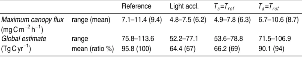
A simple global isoprene emission estimate for tropical rain forest is obtained by a temporal integration of the mean diel cycles of isoprene fluxes calculated for EUST-I and EUST-II and by spatial integration assuming a global forested area of 25

4.33 million km2 (Guenther et al., 1995). The estimated midday isoprene fluxes and total emissions are summarized in Table3. Additionally to the results obtained using the reference parameterization, the table contains model predictions for a scenario that assumes light acclimation of isoprene emission capacity (Sect.3.3). Furthermore, the

BGD

E. Simon et al. Title Page Abstract Introduction Conclusions References Tables Figures J I J I Back Close

Full Screen / Esc

Print Version Interactive Discussion

estimates are compared to predictions of two simpler approaches, assuming T_s=T_ref (isothermal surface) and T_a=T_ref (isothermal canopy layer), respectively.

The global estimate of 84 Tg C y−1 for tropical rain forest given by Guenther et al.

(1995) (hereafter referred to as G95) is at the lower end of the variability range pre-dicted by the present approach, when the reference parameterization is included in 5

the full model scheme (mean value=96 Tg C y−1). However, G95 agrees well with the mean value of the simplified isothermal surface approach, which results in a 30% re-duction of the emission budget (71.5–106.9 Tg C y−1), while the second simplification, that of an isothermal canopy layer, results in only 5% reduction (see also the calculated temperature gradients shown in Fig. 3). When the light acclimation effect is included 10

in the full model scheme, the estimate is reduced also by 30% and agrees well with G95. Potentially, the present approach contributes to a more realistic description of the emission processes, while the resulting emission estimate for isoprene remains more or less constant compared to the simpler G95 approach.

3.4. Seasonal exchange of ozone 15

In contrast to isoprene, the canopy layer represents an important sink rather than a source for ozone. As discussed in detail at the end of Sect. 2.3, chemical reactions with nitrogen oxide and other trace gases are neglected in our model calculations. A comparison of observed and predicted net fluxes and the vertical profiles of cumulative ozone deposition velocity, sink distribution and the contribution of sunlit leaves to the 20

layer sink at noon time is shown in Fig.11. Net fluxes measured above the canopy have been corrected for canopy storage (Sect.2.1). Typical observed and calculated con-centration profiles for daytime conditions are shown in Fig.12. The 14 h concentration profile is selected because daytime canopy storage is smallest in the early afternoon, which is especially important for the EUST-II data (see Fig.11d).

25

In general, the linear correlation between observed and calculated net fluxes is high

(r2>0.94). The maximum uptake occurs at noon time, when ambient concentrations

BGD

E. Simon et al. Title Page Abstract Introduction Conclusions References Tables Figures J I J I Back Close

Full Screen / Esc

Print Version Interactive Discussion

transport are low. For EUST-II, significant nighttime fluxes are observed and predicted. Interestingly, observed net deposition fluxes during EUST-I are only 50% smaller com-pared to EUST-II, whereas the levels of ambient concentrations are reduced by a factor of three to four (Table 1, Fig. 11c–d). According to Eq. (1), this must result from a seasonal variability of the dry deposition velocity v_{d ,O}

3. Since soil, aerodynamic and 5

boundary-layer resistances are very similar for both periods (for a comparison of soil resistances seeGut et al.,2002a), the variability in v_{d ,O}

3 must result theoretically from a variability of the leaf resistance to ozone uptake (r_{l eaf ,O}

3). When the same leaf pa-rameters are applied for both seasonal periods, the calculated ozone fluxes agree well with EUST-II observations but underestimate the observations for EUST-I, which are 10

double as high. Realistic physiological changes in stomatal conductances and as-similation rates are insufficient to explain this disagreement, although the differences between calculated and observed ozone deposition are reduced from 55% to 45%. The midday v_{d ,O}

3, calculated for EUST-I, increases from 0.8 to 1.05 cm s

−1

when in-creased stomatal conductance rates are applied, while the corresponding v_{d ,O}

3 for 15

EUST-II decreases from 0.85 to 0.7 cm s−1when assimilation parameters are reduced (see Table2in Sect.2.3).

A closer look on the vertical source/sink distribution shown in Fig. 11a–b indicates a potential hint for the disagreement between observed and predicted ozone deposi-tion. The shape of the source/sink distribution of ozone is more uniform compared to 20

isoprene and assimilation because the ozone uptake has a second, cuticular pathway, which is independent of physiological control (Eq. 5). The cuticular uptake is mainly controlled by the available leaf surface area and the resistance to cuticular uptake

r_cut,O

3. Therefore, the contribution of the lower canopy (0–20 m) and shaded foliage is relatively large compared to assimilation and isoprene emission. In contrast to leaf 25

surface area, where parameter uncertainty is on the order of 10% (seeSimon et al.,

2005a), the cuticular conductance (1/r_cut,O

3) is much more uncertain because it is typically small compared to stomatal conductance g_s and experimentally hard to de-termine (actually, it is not much larger than minimum g_s, g_s0). Consistent with the net

BGD

E. Simon et al. Title Page Abstract Introduction Conclusions References Tables Figures J I J I Back Close

Full Screen / Esc

Print Version Interactive Discussion

fluxes, the predicted ozone concentration profiles for EUST-II show a good agreement with observations using the value of r_cut,O

3=5000 s m

−1

, whereas EUST-I observations are strongly underestimated (Fig.12a). Reducing the cuticular resistance from 5000 to 1000 s m−1 increases the calculated fluxes for both seasonal periods by 100%. For EUST-I, this results in a good agreement between observed and calculated concen-5

trations profiles and fluxes, whereas EUST-II observations are overestimated using the lower value of r_cut,O

3.

Whereas the stomatal pathway (first part of the right side of Eq.5) has a strong max-imum in the upper canopy and occurs only at the bottom leaf side (hypo-stomatous leaves), the cuticular uptake is linearly related to the leaf area in each layer and oc-10

curs at both leaf sides (indicated by the factor of two in the second part on the right side in Eq.5). Furthermore, the stomatal pathway is coupled to physiological activity, which is much stronger in the upper canopy (Fig. 11a, b). Consequently, uncertain-ties of the stomatal pathway can not explain the disagreement between the observed and calculated ozone concentrations in the lower canopy during EUST-I. On the other 15

hand, a strong seasonal variability of r_cut,O

3 is unlikely because this implies fundamen-tal changes of leaf structure. In part, the structure and function of leaves changes as a result of lifespan regulation (Reich et al.,1991), which might be synchronized and follow the seasonal cycles of wet and dry periods within evergreen tropical rain forest. A com-bination of all the potential factors (leaf physiology, canopy and leaf structure) reduce 20

the observed disagreement between the expected and observed seasonal variability of ozone deposition, but are still insufficient. As already discussed in Sect.2.3, chem-ical sinks within the free air space are also insufficient and would affect both seasonal periods.

Speculating, we may discuss ozone deposition to wetted surfaces during EUST-I, 25

when the climatic conditions have been different. Because the relative humidity and rainfall during EUST-I were significantly higher compared to EUST-II (see Fig. 1), the ambient air in the lower canopy was nearly saturated with water vapor and large frac-tions of the leaf surfaces were wetted. The composition and chemistry of the water film

BGD

E. Simon et al. Title Page Abstract Introduction Conclusions References Tables Figures J I J I Back Close

Full Screen / Esc

Print Version Interactive Discussion

on wetted leaf surfaces are not very well understood and deposition models are treat-ing this effect on ozone uptake differently. The earliest models have considered the low solubility of ozone in pure water reducing the ozone uptake of leaves (Chameides,

1987;Baldocchi et al.,1987). However, depending on the origin and composition of the surface water, the opposite effect was also found. Larger than theoretical uptake 5

rates have been observed e.g. on leaf surfaces wetted by dew (Wesely et al.,1990) or rain water (Fuentes et al.,1992), above a deciduous forest in the winter (Padro et al.,

1992), and also over oceans (Wesely and Hicks,2000). In line with those studies, our results indicate that there might be a significant ozone uptake by wet leaf surfaces, under the likely assumption, that larger fractions of the leaf surface were wet during the 10

wet season,

3.5. Predicted response to doubled atmospheric CO₂

We investigated the physiological response of the rain forest canopy to elevated atmo-spheric CO₂ concentrations by doubling the observed CO₂ mixing ratio (resulting in 650–900 ppm at z_ref, see Fig.1a, b) and keeping all other model parameters constant. 15

The results should be interpreted with caution because important feed-backs are not considered in such a simple projection (i.e. changes in biomass, cloud cover, soil water, soil respiration, ozone chemistry etc.). Theoretically, increased CO₂levels allow leaves to maintain or even increase the substomatal CO₂ concentration with lower stomatal conductance rates. Consequently, a higher water use efficiency with higher net assim-20

ilation rates, surface temperatures and lower latent heat fluxes can be expected. The model calculated response of the rain forest is summarized in Fig.13.

On average, the model predicts a strong change in the energy fluxes and an in-crease of surface temperatures due to inin-creased atmospheric CO₂. The implied down-regulation of stomatal conductance leads to an increase of sensible heat (>24%) and a 25

decrease of latent heat, which is on the same order of magnitude. Leaf carbon uptake is increased by 22%. The changes in the surface energy budget have also an impact on the calculated isoprene emission and ozone dry deposition fluxes (calculated using

BGD

E. Simon et al. Title Page Abstract Introduction Conclusions References Tables Figures J I J I Back Close

Full Screen / Esc

Print Version Interactive Discussion

the parameterization described in Sect.2.3). Due to increasing surface temperatures, the calculated net primary emission of isoprene increases by >10% (note that leaf temperature is, besides light, the driving variable of the isoprene emission algorithm). Due to stomatal closure, the calculated dry deposition of ozone decreases, predicting a large reduction of >30%.

5

The diel cycles of the predicted increase of canopy surface temperature ∆T2×[CO2]

s,av

are shown in Fig.13b, c. The higher values predicted for EUST-II indicate an ampli-fication of the seasonal temperature differences (see Fig. 1). For EUST-I, the calcu-lated range for∆T2×[CO2]

s,av is 0.1–0.7

◦

C, whereas it is 0.3—1.0◦C for the warmer period (EUST-II). In parallel, there is an increase of 8% in the calculated sensible heat flux due 10

to increased CO₂for EUST-II compared to EUST-I, although this positive feed-back re-sponse may be partly balanced by leaf physiological changes. Assuming increased stomatal conductance rates during the wet season and decreased photosynthesis rates for the dry season, the seasonal differences become much smaller. However, this is not the case for ozone deposition. Here the model calculates very large sea-15

sonal differences in the predicted deposition change due to doubled atmospheric CO₂, which are even amplified by physiological changes, due to the strong dependence on stomatal conductance.

In general the predicted response to elevated atmospheric CO₂is very similar in kind and magnitude to what has been estimated by other modeling studies (Sellers et al., 20

1996; Leuning et al., 1998) and observed in laboratory experiments (Harley et al.,

1992;Grant et al.,1995). The long-term response of the rain forest will also depend on many different factors, which are beyond the scope of the present study, i.e. cycling of nutrients (Oren et al.,2001;Hirose and Bazzaz,1998), adaptive regulations (

Naum-burg et al.,2001), and “mega-development trends” in Amazonia (Laurance,2000). A 25

lot of experimental work will be necessary to answer these questions. However, our results demonstrate the advantage of using a coupled approach to calculate the poten-tial impact of doubled atmospheric CO₂ on the instantaneous isoprene emission and ozone deposition fluxes because the level of a priori information, required for model