Cosmological inflation : theoretical aspects and observational constraints

(1)

HAL Id: tel-01127242

https://tel.archives-ouvertes.fr/tel-01127242

Submitted on 7 Mar 2015

HAL is a multi-disciplinary open access archive for the deposit and dissemination of sci-entific research documents, whether they are pub-lished or not. The documents may come from teaching and research institutions in France or abroad, or from public or private research centers.

L’archive ouverte pluridisciplinaire HAL, est destinée au dépôt et à la diffusion de documents scientifiques de niveau recherche, publiés ou non, émanant des établissements d’enseignement et de recherche français ou étrangers, des laboratoires publics ou privés.

Cosmological inflation : theoretical aspects and

observational constraints

Vincent Vennin

To cite this version:

Vincent Vennin. Cosmological inflation : theoretical aspects and observational constraints. Cosmology and Extra-Galactic Astrophysics [astro-ph.CO]. Université Pierre et Marie Curie - Paris VI, 2014. English. �NNT : 2014PA066305�. �tel-01127242�

(2)

Th`

ese de Doctorat de l’Universit´

e Pierre et Marie Curie

Sp´ecialit´e: Cosmologie

Ecole Doctorale 127 “Astronomie et Astrophysique d’ˆIle de France” Institut d’Astrophysique de Paris

GRεCO Present´ee par Vincent Vennin

Pour obtenir le grade de

Docteur de l’Universit´e Pierre et Marie Curie

Sujet de la th`ese:

Inflation Cosmologique:

Aspects Th´

eoriques et Contraintes Observationnelles

soutenue le 5 septembre 2014 devant le jury compos´e de

M. Jérôme Martin directeur de thèse

M. Daniel Baumann rapporteur

M. Eiichiro Komatsu rapporteur

M. Michael G. F. Joyce examinateur

M. Alexei A. Starobinsky examinateur

(3)

(4)

Acknowledgements

First, I would like to express my deepest gratitude to J´erˆome Martin. First as a teacher and then as a Ph.D. director, he introduced me to the beauty of early universe cosmology and he taught me the trade of research with a lot of patience and pedagogy. I learnt a lot from his scientific rigour, his great intellectual honesty and his profund inquisitiveness. With constant support and encouragement, he offered me a very motivating and pleasant environment for doing research.

I want to thank my reporters Daniel Baumann and Eiichiro Komatsu for their patience in light of the size of this manuscript, as well as the members of my thesis jury, Michael Joyce, Aleksei Starobinsky, and Paul Steinhardt. I deeply appreciate their time and effort and I am grateful for their scientific interest in my work.

I am delighted to thank my collaborators, Robert Brandenberger, Laurence Perreault-Levasseur, Patrick Peter, Christophe Ringeval, Roberto Trotta and Jun’ichi Yokoyama with whom I worked closely and from whom I learnt a lot. I thank them for their hospitality and constant advice. Special thanks come to Christophe for having been my “computer hotline” during these three years.

I want to thank the directors of IAP, Laurent Vigroux and Francis Bernardeau, and the director of theGR"CO group, Guillaume Faye, for having provided me with ideal conditions for carrying out research, specially in a context of limited funding.

It is a pleasure to thank all those who contributed to make my work environment a very nice one: my office mates Sandrine and Charlotte, and the Salut Gorêt championship members Cédric, Jean-Philippe, Jean-Baptiste, Jérôme, Kumiko, Patrick and Stéphane. Above all, my heartfelt gratitude comes to Evaluator-IAP for teaching me interesting english expressions and for his constant encouragement in getting back to work (although I never stopped).

Finally, I want to thank my wife Doroth´ee and my baby daughter Ma¨elle for their love and support during these years and all the ones to come.

(5)

(6)

Résumé Inflation Cosmologique: Aspects Théoriques et Contraintes Observationelles

R´

esum´

e

Dans cette thèse sur articles nous nous intéressons aux contraintes observationnelles sur les modèles d’inflation cosmologique et nous étudions certains aspects fondamentaux liés à la na-ture quantique de la physique inflationnaire. L’inflation est une période d’expansion accélérée intervenant dans l’Univers primordial à très hautes énergies. En plus d’être une solution possi-ble aux problèmes du modèle standard de la cosmologie dit du “big bang chaud”, combinée à la mécanique quantique, l’inflation permet la production causale de fluctuations cosmologiques sur les grandes échelles, qui sont à l’origine des structures cosmiques actuelles. Mettant en jeu des énergies colossales au regard de ce qui peut être réalisé dans un accélérateur de particules, l’inflation est devenue un objet d’intérêt majeur en cosmologie pour tester la physique des hautes énergies au delà de son modèle standard.

Nous commen¸cons par analyser de fa¸con systématique tous les modèles inflationnaires à un champ scalaire et avec terme cinétique standard, à la lumière des mesures du fonds diffus cos-mologique les plus récentes. Dans l’approximation du roulement lent, et en intégrant les con-traintes venant de la phase de réchauffement, nous dérivons les prédictions associées à environ 75 potentiels. Nous utilisons ensuite les techniques d’inférence Bayésienne pour classer près de 200 modèles inflationnaires et contraindre leurs paramètres. Cela permet d’identifier les modèles favorisés par les observations et de quantifier les niveaux de tensions entre les différents jeux de données. L’intérêt d’une telle approche est renforcé par l’étude de méthodes indépendantes du modèle telle que le “flot de Hubble”, qui se révèle biaisé. Nous calculons également le spectre de puissance au deuxième ordre pour les modèles d’inflation-k, afin de permettre leur intégration future dans notre analyse numérique.

Dans une deuxième partie, nous décrivons certains aspects liés à la nature quantique de la physique inflationnaire. Le formalisme de l’inflation stochastique, qui incorpore les corrections quantiques aux dynamiques inflationnaires, est notamment utilisé dans le cadre du modèle à deux champs d’inflation hybride. Nous discutons l’impact de ces corrections sur les prédictions de ce modèle, et à l’aide d’un formalisme récursif, nous nous intéressons à la fa¸con dont elles modifient l’amplitude des perturbations. Finalement, la transition quantique-classique, et le problème de la mesure quantique, sont étudiés dans un contexte cosmologique. Un modèle de réduction dynamique du paquet d’onde est appliqué à la description des perturbations inflationnaires.

Mots Clés: cosmologie, inflation, fonds diffus cosmologique, inflation stochastique, inférence Bayésienne et comparaison de modèles, perturbations quantiques.

(7)

(8)

Abstract Cosmological Inflation: Theoretical Aspects and Observational Constraints

Abstract

This thesis by publication is devoted to the study of the observational constraints on cosmological inflationary models, and to the investigation of fundamental aspects related to the quantum nature of the inflationary physics. Inflation is an early phase of accelerated expansion taking place at very high energy. On top of being a solution for the hot big bang model problems, combined with quantum mechanics, inflation provides a causal mechanism for the production of cosmological fluctuations on large scales, that later give rise to today’s cosmic structures. Given that it takes place at energy scales many orders of magnitude larger than what can be achieved in conventional particle physics experiments, inflation has become of great interest to test beyond standard model physics.

We first present a systematic analysis of all single-scalar-field inflationary models with canonical kinetic terms, in light of the most up-to-date Cosmic Microwave Background (CMB) measure-ments. Reheating consistent slow-roll predictions are derived for_{⇠ 75 potentials, and Bayesian} inference and model comparison techniques are developed to arrange a landscape of _{⇠ 200} in-flationary models and associated priors. In this way, we discuss what are the best models of inflation in light of the recent observations, and we properly quantify tension between data sets. Related to this massive sampling, we highlight the shortcomings of model independent approaches such as the one of “horizon-flow”. We also pave the way for extending our com-putational pipeline to k-inflation models by calculating the power spectrum at next-to-next-to leading order for this class of models.

In a second part, we describe some aspects related to the quantum nature of the inflationary setup. In particular, we make use of the stochastic inflation formalism, which incorporates the quantum corrections to the inflationary dynamics, in the two-field model of hybrid inflation. We discuss how the quantum diffusion can affect the observable predictions in such models, and we design a recursive strategy that incorporates its effects on the perturbations amplitude. Finally, we investigate the quantum-to-classical transition and the quantum measurement problem in a cosmological context. We apply a dynamical wavefunction collapse model to the description of inflationary perturbations.

Keywords: cosmology, inflation, cosmic microwave background radiation, stochastic inflation, Bayesian inference and model comparison, quantum perturbations.

(9)

(10)

Introduction

Inflation is a phase of accelerated expansion that took place in the early Universe at very high energy. Originally intended to dispose of some of the hot big bang shortcomings, it was soon realized that inflation may be responsible for a powerful manifestation of our Universe’s quantum nature. Indeed, the deviations from homogeneity and isotropy that give rise to today’s cosmic structures (galaxies, clusters, filaments, etc.) can be traced back to the quantum fluctuations of gravitational and matter fields during inflation. Stretched by the quasi-exponential expansion of space-time to distances of cosmological interest today, these fluctuations serve as the primordial seeds for inhomogeneities that later grow under the influence of gravitational instability. Inflation has become a very active field of research in the past years, since the energy scales involved during this early epoch are many orders of magnitude greater than those accessible in particle physics experiments. Therefore, the early Universe is certainly one of the most promising probes to test beyond standard model physics.

Another consequence of the fact that inflation takes place at energy scales where particle physics remain unknown, is that the physical nature of the fields driving inflation, and their relation with the standard model of particle physics, is still unclear. There have been a crowd of inflationary candidates proposed so far, and an important task is to discriminate between them. On the other hand, there is now a flow of increasingly accurate astrophysical data which provides us with a unique opportunity to constrain the inflationary landscape. These data mostly consist in measurements of the Cosmic Microwave Background (CMB), but they also concern other astrophysical probes such as supernovae, galaxy surveys, and 21 cm observations. It becomes therefore of paramount importance to be able to process such a huge amount of observational data, comprising measurements that are very different in nature, with hundreds of inflationary scenarios, often equally different. It is the first purpose of this thesis to design scientific and technical tools enabling to carry out such a programme, and to determine which inflationary models the data seem to prefer.

At the fundamental level, inflation is also probably one of the only cases in physics where an effect based on General Relativity and Quantum Mechanics leads to predictions that, given our present day technological capabilities, can be tested experimentally. This makes inflation an ideal playground to discuss deep questions related to its quantum aspects. The other purpose of this thesis is to study some of them, ranging from the quantum-to-classical transition of cosmological perturbations, to the quantum corrections to the inflationary dynamics by means of the stochastic inflation formalism.

The present manuscript is a thesis by publication. It presents the works realized at the Institut d’Astrophysique de Paris between September 2011 and September 2014 under the direction of J´erˆome Martin. It first contains a brief presentation of the cosmological groundwork for our analysis, which introduces the main aspects of the cosmological standard model and of inflation. Mainly, this part I aims at providing the reader with the conceptual and technical tools that may be helpful to the understanding of the results presented in partII. This second part collects the research articles published during this thesis time (except from section 3.4 which, at the

(11)

Introduction

time of drafting this manuscript, is going through the reviewing process).

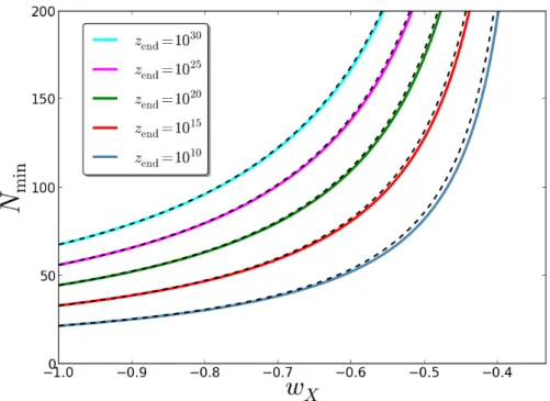
More precisely, this document is organized as follows. In chapter 1, we review the cornerstones of the standard model of modern cosmology. In the framework of General Relativity, we describe homogeneous and isotropic universes and derive the associated Einstein equations. By an ex-plicit comparison with the corresponding Newtonian physics, we highlight the deeply relativistic nature of the expansion, especially its possible acceleration. We then give a brief description of the main constituents of the Universe, and of the main lines of its history. Finally, we turn to the presentation of the problems of the hot big band model, namely the horizon, flatness and monopole problems. For each of these problems, we give a detailed calculation of its formula-tion and show how it can be solved with a phase of accelerated expansion. In particular, we characterize the number of e-folds that is required in each case.

In chapter 2, we review some aspects of cosmological inflation, the physical setups it relies on, the predictions it makes and the fundamental issues it raises. We explain why and under which conditions a single scalar field can support a phase of inflation and we present the “slow-roll” approximation which enables to solve its dynamics perturbatively. It also provides us with a convenient frame of calculation to compare inflationary predictions with observational data, which we make widely use of in chapter 3. We then turn to the description of inflationary perturbations, and show how cosmological fluctuations need to be quantized. For illustrative purpose, we provide a detailed calculation of the power spectrum of scalar perturbations, at first order in slow roll. Finally, we devote a large part of this second chapter to the presentation of the stochastic inflation formalism which is used in chapter 4. We first present a detailed heuristic derivation of the Langevin equation which is at the heart of this formalism, before turning to the question of the time variable that should be used when solving such equations, in order to reproduce results from Quantum Field Theories. Lastly, we address the issue of the calculation of physical observable quantities in stochastic inflation, such as the power spectrum of adiabatic perturbations. We show that the stochastic setup allows to reproduce the standard result, before providing complete solutions which do not rely on an expansion in the noise term. To our knowledge, this is the first time that such a non perturbative calculation of the power spectrum in stochastic inflation is presented. It has not been pre-printed or published yet since it has been derived in the course of drafting this manuscript.

We then turn to part II where the articles published during this thesis are presented and dis-played. The first chapter, chapter3, deals with a systematic analysis of all single-field inflation-ary models with minimal kinetic terms, in light of the most up-to-date CMB data, especially the ones coming from the Planck experiment and more recently from BICEP2. This somewhat “industrial” project aims at deriving reheating consistent slow-roll predictions for _{⇠ 75} infla-tionary potentials, and using Bayesian inference and model comparison techniques to arrange a landscape of _{⇠ 200 inflationary models and well studied priors. In this way, one can discuss} which are the best models of inflation. This also allows us to assess the compatibility level of the two data sets (Planck and Bicep2) given inflation, or given a specific inflationary model. The relevance of such an approach is further advocated for in an article pointing out the shortcom-ings of model independent parametrizations of inflation such as the one of “horizon flow”, and another one paves the way for including single field k-inflation (i.e. non minimal kinetic terms) models in our analysis, by calculating the power spectrum at next-to-next-to leading order for this class of models.

In chapter 4, we turn to the description of some aspects related to the quantum nature of the inflationary setup. In particular, the stochastic inflation formalism incorporates the quantum corrections to the inflationary dynamics by means of stochastic Langevin equations. This gives

(12)

rise to non trivial inflationary trajectories, especially when multiple fields are present. This is why we study stochastic effects in hybrid inflation, a two-field model where inflation ends by tachyonic instability, and we discuss how the quantum diffusion can affect the observable predictions in such models. Making use of a recursive formalism for backreacting effects, we also address the issue of evolving cosmological perturbations on top of stochastically shifted backgrounds, in the same type of models. Finally, we investigate the quantum-to-classical transition and the quantum measurement problem in a cosmological context. More precisely, we apply the continuous spontaneous localization modification of the Schr¨odinger equation to the case of inflationary perturbations. We establish what an efficient collapse of the wavefunction implies for the inflationary predictions, and which constraints can be derived on the collapse models themselves.

Finally, in a last section, we sum up our results and present some concluding remarks and possible prospects for the present work.

(13)

(14)

Part I.

Cosmology and Inflation

(19)

(20)

1. The Cosmological Standard Model

In this chapter, we review the cornerstones of the standard model of modern cos-mology. The Hot Big Bang scenario describes a series of events that occurred since an initial singularity 13.7 billion years ago, and for which we now have accurate ob-servational evidence. Questions left unanswered by this model are discussed, which are solved by the introduction of an era of accelerated expansion in the early Uni-verse. In this section, only a brief and partial overview of the standard cosmological model is given, the various aspects of which are further detailed in a broad range of textbooks [1, 2, 3, 4, 5, 6, 7, 8].

Considerations about the extent and the structure of the Universe exist in almost every culture and seem to be intrinsic to the development of human awareness. In this sense, Cosmology is a matter of concern which may be considered as old as mankind itself. However, for a very long time, it consisted in a very speculative approach to metaphysical (more than physical) issues in which philosophy or even religion were also at stake. This radically changed only in the first half of the twentieth century with the advent of the theory of general relativity, which provided for the first time a mathematical consistent framework for describing space and time. Cosmological models, in which space is expanding, were derived from this theory and enabled to understand many observations starting with galaxies receding. During these years, Cosmology was mainly about describing and reconstructing a posteriori observational effects of this expansion. Then, in the second half of the twentieth century, was formulated the hot big bang model, which includes the description of physical processes occurring in this expanding space-time, and the associated thermal history of the Universe. More recently, Cosmology has entered a precision era with the inflow of high accuracy observational data such as the Cosmic Microwave Background (CMB) measurements, galaxy and supernova surveys, 21 cm astrophysics data, forthcoming cosmic rays and gravitational waves detectors, etc. Together with theoretical developments in high energy and gravitational physics, this enabled to upgrade Cosmology to the status of a genuine Science, i.e. a field of research in which falsifiable predictions can be made and tested.

1.1. The Homogeneous and Isotropic Universe

The distribution of galaxies and cosmological structures in space around us appears to be isotropic on large scales [_{⇠ O(100) Mpc] , which implies that space-time possesses a} spher-ical symmetry around us. This observational fact, combined with the Copernican principle1

which states that we should not live in a central or specially favoured position in the Universe, leads to the conclusion that the Universe must be homogeneous on large scales. This is the

1_{The Copernican Principle is to be understood as opposed to the anthropocentrist view that human beings}

should be at the center of the Universe. For example, the Aristotelian model of the solar system in the Middle Ages placed the Earth at the center of the solar system, a unique place since it “appeared” that everything revolves around the Earth. Nicolaus Copernicus demonstrated that this view was incorrect and that the Sun was at the center of the solar system with the Earth in orbit around the Sun.

(21)

Chapter 1. The Cosmological Standard Model

Figure 1.1.: Hubble diagram (i.e. velocity against distance) for extra-galactic nebulae, from the 1929 original paper [13] by Edwin Hubble. Such diagrams lead to the hypothesis of an expanding universe with a linear expansion law v = Hr. The radial velocities are obtained from redshift measurements and are corrected for solar motion, and distances are estimated from involved stars and mean luminosities of nebulae in a cluster. The black discs and full line represent the solution for solar motion using the nebulae individually; the circles and broken line represent the solution combining the nebulae into groups; the cross represents the mean velocity corresponding to the mean distance of 22 nebulae whose distances could not be estimated individually.

so-called cosmological principle.

1.1.1. The Friedmann-Lemaˆıtre-Robertson-Walker Metric

The cosmological principle is a statement about the amount of symmetry present in the observ-able Universe. As always in physics, this symmetry constrains and simplifies the mathematical description of the system under consideration. In this manner, under the cosmological principle symmetry, the metric of space-time ds2 = gµ⌫dxµdx⌫ can be shown to be entirely determined up to a free function of time, the scale factor a(t), and a discrete parameterK = −1, 0, 1 which encodes the spatial curvature (open, flat or closed). With the (_{−, +, +, +) signature convention,} it is of the form [9,10,11,12] ds2 =_−dt2+ a2(t)  dr2 1− Kr2 + r 2_"d✓2_{+ sin}2_✓dφ2# $ (1.1) and is called the Friedmann-Lemaˆıtre-Robertson-Walker (FLRW) metric. In this parametriza-tion, t is the cosmic time, r is the comoving radial coordinate which is unitless, ✓ and φ are the comoving angular coordinates, and a(t) has units of length.2

1.1.1.1. The Hubble Law

From the FLRW metric (1.1), one can see that the physical distance Lphys between two points measured on a constant t hypersurface scales as the scale factor a, that is to say

Lphys = a(t)Lcom, (1.2)

2_{Hereafter and unless stated otherwise, we work in the unit system where c = ~ = k} B= 1.

(22)

1.1. The Homogeneous and Isotropic Universe

Figure 1.2.: Comparison of H0 measurements, with estimated of ±1σ errors, from a number of different astrohphysical techniques, and compared with the spatially-flat ΛCDM model constraints from Planck and WMAP9. Image Credit: Ref. [15].

where Lcom is the so-called comoving distance, which is constant in time for still objects in the FLRW frame. The scale factor a thus sets the overall expansion (or contraction) level of space hypersurfaces, hence its name. Another consequence of the FLRW metric is a linear relation between distance and velocity. Indeed, from differentiating Eq. (1.2) with respect to cosmic time t, one obtains

v = dLphys dt =

˙a

aLphys = HLphys, (1.3)

where we have defined the Hubble parameter H⌘ ˙a/a. This is the so-called Hubble law. It was first observed in 1929, as presented in Fig.1.1, where the current value of H, that we denote H0, was determined to be of the order of 500 km/sec/Mpc. As we will see below, this value contains valuable information about the content of the Universe and this is why it has been the object of much research effort. The first good estimation was realized in 1958 in Ref. [14], where the value 75 km/sec/Mpc was obtained. Finally, the most up to date measurements provided by the Planck mission [15] gave the value 67.80± 0.77 km/sec/Mpc for the value of H0. This value is rather low compared with previous measurements, see Fig. 1.2, and the tension between the CMB-based estimates in the ΛCDM model and the astrophysical measurements of H0 is still intriguing [15,16,17,18,19,20,21].

The reduced Hubble parameter h is also often used, and is defined as

H0 = 100 h km/sec/Mpc . (1.4)

The Hubble parameter sets the fundamental physical scale of space-time. It provides a charac-teristic time scale H₀−1 ' 4.551 ⇥ 1017_{sec called the “Hubble time” and a characteristic length} scale H₀−1 _{' 1.364 ⇥ 10}26m called the “Hubble radius”. As we will see later, the Hubble time sets the scale for the age of the Universe, and the Hubble length sets the scale for the size of the observable Universe. These values are displayed in table 1.2 where we collect all the numerical values given and used throughout this section 1.

(23)

Chapter 1. The Cosmological Standard Model 1.1.1.2. Redshift and Comoving Coordinates

Another interesting property of FLRW space-times is that light gets redshifted as its travels, due to the time dependence of the scale factor. Let us consider an emitting object at rest in the comoving coordinates system, with radial coordinate r1, while an observer is located at r0= 0. Light is emitted from this first object at time t1 with frequency ⌫1, and received by the observer at time t0with frequency ⌫0. Let us determine the relation between ⌫0and ⌫1. Since light travels along geodesics with ds = 0, radial light path traveling towards the observer (d✓ = dφ = 0 and dr/dt < 0) follows dt a (t) = dr p 1− Kr2. (1.5)

Now consider the emission of two subsequent crests of a light wave. The first one is emitted at (t1, r1) and received at (t0, 0) while the second one is emitted at (t1+ δt1, r1) and received at (t0+ δt0, 0). From Eq. (1.5), one has

Z 0 r1 dr p 1_{− Kr}2 = Z t₀ t1 dt a(t) = Z t₀+δt₀ t1+δt1 dt a(t). (1.6)

Subtracting the third integral from the second, in the limit δt0, δt1 ⌧ a/ ˙a, one obtains δt0

a (t0)

= δt1 a (t1)

. (1.7)

Since the time delay δt between two crests is nothing but the inverse frequency, one obtains ⌫1

⌫0

= a (t0) a (t1)

= 1 + z , (1.8)

where the last equality defines the redshift z. This quantity only depends on the ratio of the scale factor at reception to the scale factor at emission.

In terms of wavelength λ, Eq. (1.8) gives λ0/λ1 = a(t0)/a(t1). We see that the wavelength of light just contracts and stretches with the scale factor λ _{/ a. Another way to look at this is} to say that a photon traveling through an FRLW space-time loses momentum as the Universe expands,

p = h⌫ _{/ a}−1(t) . (1.9)

As shown in appendix 1.A, see Eqs. (1.95) and (1.96), this momentum loss applies to massive particles as well as photons, and any particle moving in an expanding FLRW space-time loses momentum as p_{/ a}−1. This means that a massive particle asymptotically comes to rest relative to the comoving coordinates system. Thus, comoving coordinates represent a preferred reference frame which is such that any free body with a peculiar velocity relative to the comoving frame eventually comes to rest in this frame.

1.1.1.3. Einstein Equations

The Einstein-Hilbert action [22,23,24] describes the dynamics of space-time metrics, and reads Sgrav = 1 2 Z d4xp_{−g (R − 2Λ) ,} (1.10) where  ⌘ 8⇡G = 8⇡/m2

Pl = 1/MPl2, where G is the Newton gravitational constant, mPl is the

Planck mass and MPl ' 2.4 ⇥ 1018 GeV is the reduced Planck mass. In the above expression,

(24)

1.1. The Homogeneous and Isotropic Universe Λ is a cosmological constant, g is the determinant of gµ⌫ and R is the Ricci curvature scalar R⌘ gµ⌫_R

µ⌫. It is constructed from the Ricci tensor Rµ⌫ = 2Γ⇢_µ[⌫,⇢]+ 2Γ⇢_λ[⇢Γλ_⌫]µ, where brackets mean anti-symmetrization over the indices and where the Christoffel symbols are given by Γ⇢µ⌫ =

1

2g⇢λ(@⌫gλµ+ @µgλ⌫− @λgµ⌫).

To this action should be added a part Smatter = R Lmatterp−gd4x describing matter in the Universe. When varying these two action terms with respect to gµ⌫, one obtains two tensors, namely the Einstein tensor Gµ⌫ defined as

Gµ⌫+ Λgµ⌫ ⌘ p2 −g @Sgrav @gµ⌫ = Rµ⌫−1 2Rgµ⌫+ Λgµ⌫ (1.11)

for the gravity part, and the energy-momentum tensor Tµ⌫ ⌘ − 2 p −g @_Smatter @gµ⌫ = gµ⌫Lmatter− 2 δ_Lmatter δgµ⌫ (1.12)

for the matter part. This leads to the well-known Einstein equations

Gµ⌫+ gµ⌫Λ = Tµ⌫. (1.13)

Let us now work out the two tensors Gµ⌫ and Tµ⌫ for an FLRW metric. When the metric (1.1) is plugged into the definition (1.11), one obtains (a detailed calculation is provided in appendix

1.A) G00= 3 ✓ H2+ K a2 ◆ , Gij =− ✓ H2+ 2¨a a+ K a2 ◆ gij, (1.14) where the index 0 is for time t, and the indexes i and j are for space coordinates so that gij is just the spatial part of the full metric gµ⌫.

Given the symmetries of space-time, one can show that the most generic form of the energy-momentum tensor is given by

Tµ⌫ = ⇢uµu⌫+ p

a2gµ⌫, (1.15)

where gµ⌫ = gij when µ and ⌫ are space indexes and 0 otherwise. In the above expression, ⇢ and p are two constants depending on time only, and uµ is the four velocity of a comoving observer for whom space is homogeneous and isotropic. One thus has uµ= δµ,0, where δ is the Kr¨onecker symbol. Since p is associated to the spatial part of the tensor, it can be interpreted as the pressure of matter, while ⇢ = Tµ⌫uµu⌫ is the energy density measured by a comoving observer. The above form of Tµ⌫ is entirely fixed by the cosmological principle. Finally, let us mention that the time component of the conservation relation rµTµ⌫ = 0 leads to

˙⇢ + 3H (⇢ + p) = 0 . (1.16)

Heuristically, this equation can be understood as a translation of the first law of thermodynamics, dU =_{−pdV , with U = ⇢V and V = a}3_.

1.1.2. An Expanding Universe

Let us now detail how this general relativistic framework allows to relate the dynamics of the expansion of space-time to the matter content properties of the Universe.

(25)

Chapter 1. The Cosmological Standard Model 1.1.2.1. Friedmann and Raychaudhuri Equations

If one plugs the above expressions for Gµ⌫, Eqs. (1.14), and for Tµ⌫, Eq. (1.15), in the Einstein equation (1.13), one obtains the two following dynamical equations

H2 =  3⇢− K a2 + Λ 3 , (1.17) ¨ a a = −  6(⇢ + 3p) + Λ 3 . (1.18)

These two equations are known as the Friedmann [25] and the Raychaudhuri [26] equations, respectively. Because of the Bianchi identities, when combined together, one can check that they account for the conservation equation (1.16).

The Friedmann equation relates the change of the scale factor of the Universe to its energy density, spatial curvature and cosmological constant. If the Universe is assumed to be flat (_{K = 0) and if the cosmological constant vanishes (Λ = 0), this means that the only presence} of energy will cause the Universe to expand (H > 0) or to contract (H < 0). In the following, we shall mostly consider expanding universes, even if contracting universes are key ingredients of some cosmological models [27,28,29,30,31,32,33,34].

From the Raychaudhuri equation, one can notice that in absence of a cosmological constant, any form of matter such that ⇢ + 3p < 0 will cause an acceleration of the scale factor ¨a > 0 if it dominates the energy budget of the Universe. The energy density is always positive, but in some cases the pressure can be negative and the inequality ⇢ + 3p < 0 may be realized. This simple property is deeply rooted in the inflationary scenario and will be discussed in more details in chapter 2. As we shall now see, it is intimately related to the fundamental principles of general relativity.

1.1.2.2. The Newtonian Expanding Sphere

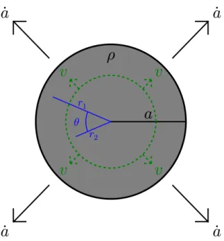
In order to highlight the relativistic effects in the above setup more clearly, let us derive the Newtonian version [35, 36, 37] of the Friedmann and Raychaudhuri equations. In Fig. 1.3, we sketch the case of an expanding sphere of radius a filled with uniform matter with mass density ⇢. Let us consider a particle of mass m sitting on the out-shell of this sphere. The Gauss theorem states that the gravitational attractive force seen by such a particle is given by GmM/a, where M = 4/3⇡⇢a3 is the integrated mass of the sphere. Its acceleration being simply ¨a, the second Newton law gives rise to m¨a =_{−MGm/a, i.e.}

¨ a a ) ) ) ) Newton =−4 3⇡⇢G =−  6⇢ . (1.19)

This matches the Raychaudhuri equation (1.18) without cosmological constant and without the pressure term. This is why in Newtonian mechanics, one must have ¨a < 0 and the expansion of the sphere can only decelerate. The reason why acceleration is allowed in the general relativistic setup is because all forms of energy gravitate, including pressure.3 As a consequence, the presence of pressure in the Raychaudhuri equation is a crucial signature of the relativistic nature

3_{Acceleration of FRLW space-times is actually one of the only manifestations of pressure’s self-gravity [}₃₈_],

otherwise tested only in the context of big bang nucleosynthesis [39] where it is necessary to account for current light element abundances. For example, even in compact objects such as neutron stars, pressure’s self-gravity is immeasurable given uncertainties on the equation of state [40,41].

(26)

Figure 1.3.: Homogeneous sphere in Newtonian radial expansion.

of the setup. Indeed, in newtonian mechanics, masses source the gravity field, but relativity relates mass to energy. Since energy is not a relativistic invariant but mixes up with momentum when changing frames, momentum, hence pressure, naturally comes into play in a relativistic context.

It is also interesting to calculate the newtonian energy ENewtonof the sphere of Fig.1.3. In order to do this, we first need to derive the velocity profile v(r) of the sphere radial expansion. When diluting, let us assume that the mass density scales as the inverse of the volume to some power 1 + w, ⇢/ V−(1+w) _{(where for ordinary “newtonian” matter, w = 0). One can first show}4 _that

its evolution is given by

˙⇢ =− (w + 1)  v0(r) + 2v (r) r $ ⇢ . (1.20)

In order for the sphere to remain homogeneous (i.e. to be such that ⇢, hence ˙⇢, does not depend on r), the term factorizing ⇢ in the right hand side of the previous relation should not depend on r, i.e. one must have v0+ 2v/r = constant. This leads to the two-branch solution

v (r) = Ar + B

r2 (1.21)

for the radial velocity, where A and B are two integration constants that can only depend on time. In this manner the sphere is and remains homogeneous. However, there is no reason why it should be isotropic. Indeed, even if the sphere is taken to be infinite, the direction pointing towards its center is a priori a privileged direction. This is not the case only if the velocity law (1.21) v(r) is valid not only for r being the distance between the center of the sphere and one of its shells, but for r being the distance between any two points within the sphere. As we shall now see, this selects out one of the two branches of the solution (1.21). Let us thus consider

4_{Two shells of radius r}

1 and r2 = r1+ dr respectively become, after a dt long expansion, two shells of radius

r0

1 = r1+ v(r1)dt and r02 = r1+ dr + [v(r1) + v0(r1)dr] dt. The volume contained between these two shells

thus evolves from V = 4⇡r12dr to V 0 = 4⇡r0 12(r 0 2− r 0 1) ' V [1 + 2v(r1)/r1dt + v 0

(r1)dt]. From here one gets

dV /dt = V (v0

+ 2v/r), and with ⇢Vw+1_{= constant, Eq. (}_1.20_).

(27)

two points of radial distances r1 and r2respectively, and with angular separation ✓ as in Fig.1.3. The distance between these two points is simply given by d12=pr2₁+ r2₂− 2r1r2cos ✓. Since ✓ is conserved through the radial expansion, its time variation is

˙ d12=

r1v (r1) + r2v (r2)− [r2v (r1) + r1v (r2)] cos ✓ d12

. (1.22)

On the other hand, if the velocity law (1.21) is isotropic, one must have ˙

d12= v (d12) . (1.23)

When the velocity law (1.21) is used in the identification of Eqs. (1.22) and (1.23), it is straight-forward to see that B = 0. Only the first branch remains, and one has

v (r) = Hr , (1.24)

where we have renamed H _{⌘ A = ˙a/a = ˙r/r, which can only depend on time. In a cosmological} context, one recovers the Hubble law previously mentioned. In particular, it is in order to stress that it eventually does not depend on the volume scaling power index w.

We are now in a position where we can calculate the energy of the sphere. It is given by the sum of its integrated kinetic energy and its integrated potential energy, that is

ENewton = Z a 0 1 2(4⇡r 2_dr⇢)(rH)2₋Z a 0 G r "4⇡r 2_dr⇢#✓ 4 3⇡r 3_⇢ ◆ = 2 5⇡⇢a 5_H2₋16⇡2 15 G⇢ 2_a5 = 2 5⇡a 5_⇢⇣_H2₋  3⇢ ⌘ . (1.25)

Remembering that ⇢ scales as V−(w+1) / a−3(w+1)_{, one obtains} H2 =  3⇢ + 5ENewton 2⇡⇢0a3(w+1)0 1 a2−3w . (1.26)

When the Newtonian energy vanishes, one obtains the Friedmann equation (1.17) in absence of cosmological constant and curvature, the presence of which is therefore a truly relativistic effect. In passing, let us notice that when ENewton6= 0 and for ordinary matter (such that w = 0), the second term in the right hand side of Eq. (1.26) plays a role similar to the one of curvature in Eq. (1.17), which scales as a−2 and which can be either positive or negative.

A last remark is in order about the conservation equation. In Newtonian mechanics, if one replaces v(r) = Hr in Eq. (1.20), one obtains the conservation equation ˙⇢ + 3(w + 1)H⇢ = 0, which, in passing, matches Eq. (1.16) if p = w⇢. This relation is fairly trivial since it just states that ⇢_{/ V}−(1+w). Thanks to this conservation law, one can check that the two equations (1.19) and (1.26) are actually equivalent when w = 0. This is just a consequence of the fact that the conservation of mechanical energy is equivalent to the second Newton law, i.e. that Newtonian mechanics derives from a potential. However, in the case of general relativity, the conservation equation (1.16) is not trivial at all and is required to relate the Friedmann and Raychaudhuri equations. One thus really have two independent dynamical equations.

(28)

fluid equation of state parameter w ρ(a) a(t)

cold matter 0 _{/ a}−3 _{/ t}2/3

radiation 1/3 _{/ a}−4 _{/ t}1/2

spatial curvature _−1/3 _{/ a}−2 _{/ t}

cosmological constant ₋₁ _{/ a}0 _{/ exp (Ht)}

scalar field _{−1 + 2✏}1/3 / a−2✏1 t1/✏1

Table 1.1.: Equation of state parameter w for a few fluid examples, with corresponding ⇢(a) (1.27) and a(t) (1.30) profiles.

1.1.2.3. Constant Equations of State

It is interesting to notice that the conservation equation (1.16) can be solved in the simple case of a single ideal fluid where the energy density and the pressure are related by a constant equation of state parameter w_{⌘ p/⇢. One obtains}

⇢= ⇢in ✓ a ain ◆−3(1+w) . (1.27)

The equation of state parameter of cold matter is simply wmat = 0 so that the energy density scales as the inverse volume ⇢mat / a−3, while the equation of state parameter of radiation is wrad = 1/3 so that the associated energy density scales as ⇢rad / a−4, which includes both volume dilution effect (/ a−3_{) and wavelength redshift (}_1.8_{) (}_{/ a}−1_{). From the Friedmann} equation (1.17), one can also associate an energy density to curvature ⇢K⌘ −3K/(a2) and to the cosmological constant ⇢Λ⌘ Λ/, so that the Friedmann equation reads

H2 = 

3(⇢matter+ ⇢K+ ⇢Λ)⌘ 

3⇢T, (1.28)

where ⇢_T denotes the “total” energy density. Here, ⇢matter can include ordinary cold matter, radiation, or any other Universe constituent. Since ⇢K/ a−2, this means that curvature can be viewed as a fluid constituent with equation of state parameter wK=−1/3. In the same manner, ⇢Λ is constant and can be viewed as a fluid constituent5 with equation of state parameter wΛ=−1. These values for the equation of state parameters are summarized in table 1.1. The last entry corresponds to a scalar field and will be further explicated in chapter 2.

Interestingly enough, since pΛ= wΛ⇢Λ=−⇢Λ, the Λ/3 term in the right hand side of Eq. (1.18) can also be written_−/6(⇢Λ+3pΛ). In the same manner, since pK=−⇢K/3, adding a−/6(⇢K+ 3pK) = 0 to the right hand side of Eq. (1.18) does not change it, so that similarly to Eq. (1.28), the Raychaudhuri equation can be written as

¨ a a =−  6 [⇢matter+ ⇢Λ+ ⇢K+ 3 (pmatter+ pΛ+ pK)] =−  6(⇢T+ 3pT) , (1.29)

where p_T denotes the “total” pressure. This is why, as far as the two dynamical equations (1.17) and (1.18) are concerned, the curvature can be viewed as an ideal fluid constituent with equation

5_{This should not come as a surprise since the conservation relation r}

µTµν = 0 is invariant under the redefinition

Tµν ! Tµν+ Λgµν. This is the reason why a cosmological constant can actually be thought of as being part

of the matter side of the Einstein equations.

(29)

of state parameter wK = −1/3 and the cosmological constant can be viewed as an ideal fluid constituent with equation of state parameter wΛ=−1.

If the scale factor a evolves monotonously with time, the right hand side of the Friedmann equation (1.28) soon gets dominated by a single fluid (the one with the smallest w if space expands, or the one with the largest w if space contracts). In this limit, it can be integrated, leading to a (t) = 8 > > > < > > > : ain  1_±3 2(1 + w) r ⇢in 3 t_{− t}in MPl $_3(1+w)2 if w_{6= −1} ainexp ✓ ±r ⇢₃int_M− tin Pl ◆ if w =₋₁ , (1.30)

where ain and tin are two integration constants. The sign ± depends on whether space is expanding (plus sign, H > 0) or contracting (minus sign, H < 0). In what follows, only the case of an expanding space will be considered. The ⇢(a) shape (1.27) and the a(t) shape (1.30) are also given in table 1.1for the fluids mentioned so far.

Finally, it is interesting to notice that the conservation equation (1.16) can also be integrated when the Universe is made of a collection of ideal independent fluids with equations of state wi= pi/⇢i. In this case indeed, the conservation equation gives rise to

X i

[ ˙⇢i+ 3H (1 + wi) ⇢i] = 0 . (1.31)

One of the solutions is of course when all the terms of the above sum vanish. Physically, this corresponds to a situation of non interacting independent fluids, where there is no energy transfer from one fluid to another. Obviously, in this case the scaling solution (1.27) applies for all the fluids, and the total energy density is given by

⇢_T =X i ⇢in_i ✓ a ain ◆−3(1+wi) . (1.32)

Unfortunately however, in this case the Friedmann equation H2 = ⇢_T/3 cannot be integrated analytically.

1.2. The Present Composition of the Universe

Thanks to Eq. (1.32), we now know how the energy density of each constituent of the Universe evolves with time, at least provided its equation of state parameter is constant. Therefore, up to potential energy transfer between constituents, it is enough to know the energy densities at a single time (most conveniently, now) to derive their value at any other time. This is why we now discuss the present composition of the Universe.

To this end, we first define the critical density ⇢crit with respect to the Hubble parameter,

⇢crit=

3 H

2_. _(1.33)

The total energy density ⇢totis the sum of all contributions but the curvature one, ⇢tot = ⇢T−⇢K.

If one writes ⇢tot=Pi⇢i, each part ⇢i stands for an ideal fluid i with its own equation of state

(30)

1.2. The Present Composition of the Universe

Figure 1.4.: Current Energy Composition of the Universe.

parameter wi. The dimensionless quantities Ωi = ⇢i/⇢crit then allow to re-write the Friedmann

equation (1.28) simply as

Ωtot = X

i

Ωi = 1− ΩK, (1.34)

where we stress again that the curvature term (which, contrary to the others, can be either positive or negative) is treated separately. In the present Universe, the components contributing to this relation have the following weights.6

Radiation

Most of the photons present in the Universe belong to the Cosmic Microwave Background, see section 1.3.3. They represent a tiny fraction of ⇢tot, with [15] Ω(0)_rad⇡ 9.3 ⇥ 10−5.

Baryonic Matter

The contribution from ordinary matter (i.e. the one we find in atoms, nuclei, etc.) to Ωtot is dominated by cold baryons (strongly interacting composite subatomic particles made up of three quarks) which are much heavier than leptons (elementary spin 1/2 particles that do not undergo strong interaction, such as electrons or neutrinos). However, they only amount to [15] Ω(0)_b ⇡ 0.049.

Nonbaryonic (or “Dark”) Matter

In order to consistently explain many observational facts, ranging from galaxy rotation curves and large scale structure formation to the CMB statistics, it is common to postulate the existence of another non-relativistic matter component in the Universe, with w = 0 as well, referred to as “dark matter”. Its current contribution is [15] Ω(0)_dm_{⇡ 0.268 and therefore, it strongly dominates} over ordinary matter. The nature of dark matter is obviously the subject of active study.

6_{All quantities referring to their current (present-day) value are designated by a subscript (or occasionally a}

superscript) “0” or “(0)”.

(31)

Chapter 1. The Cosmological Standard Model Curvature

When _{K = 0, the Universe is globally flat. If K = ±1 however (K = 1 corresponds to a} closed universe while K = −1 corresponds to an infinite universe), there should be a curvature component in the current Universe energy budget. However, it has not been detected yet, and all the observations made so far are still consistent with Ω(0)_K _{' 0. The current constraints give [}15] 100Ω(0)_K =−0.10+0.62−0.65 at 95% confidence level.

Dark Energy

Evidently, after summing over radiation, baryonic and non-baryonic matter, the bulk part of the Universe’s energy density is still missing. Together with evidence from a recent acceleration in the expansion of the Universe, this motivates the introduction of a missing fluid named “dark energy”, with an equation of state parameter w_{' −1. This is why the cosmological constant Λ} (for which w =_{−1 exactly) is one of the candidates for dark energy, even if as for dark matter,} the nature of dark energy is the subject of active study (for a nice review, see Ref. [42]). It accounts for the major contribution to Ω(0)_tot, i.e. [15] Ω(0)_de _{⇡ 0.683 .}

The values mentioned here are given in table1.2. The relative contributions of these constituents is also displayed in Fig.1.4. One can see that the Universe is currently dominated by fluids the physical nature of which is still not well understood (dark matter and dark energy). This gives us an idea of the theoretical effort still needed to build a complete and standard description of cosmology.

1.3. The History of the Universe: the Hot Big Bang Model

In the previous section, we have stated the current values of the energy fractions Ω(0)_i for the Universe main components. Combined with the dynamical considerations of section 1.1.2, this enables us to now infer the main lines of the history of the Universe.

1.3.1. Dominant Constituant

Plugging the previously given values for Ω(0)_i in Eq. (1.32), ⇢tot/⇢cri = P_iΩ(0)_i (a/a0)−3(1+wi), allows us to discuss the way ⇢tot varies with a. The result is displayed in the left panel of Fig. 1.5. The black dashed line stands for the total sum, while the coloured lines follow each of its components. Because of the different scalings with a, each component of the Universe dominates its content at a different epoch (called “eras” in what follows).

The Universe is currently dominated by dark energy which means that ⇢tot ' constant. Since cold matter ⇢mat⌘ ⇢dm+ ⇢b scales as a−3, its contribution increases when moving backwards in time and becomes larger than the one of dark energy at some point aaccdefined by ⇢mat(aacc) = ⇢de(aacc), i.e. aacc/a0 =

h

Ω(0)_mat/Ω(0)_dei1/3. Here, the subscript “acc” stands for the onset of the dark energy phase.7 _{When a < a}

acc, the Universe is dominated by cold matter and one has

7_{One should note that contrary to what the notation may suggest, acceleration of the expansion does not begin}

(32)

1.3. The History of the Universe: the Hot Big Bang Model

Figure 1.5.: Left panel: energy density (1.32) of the Universe constituents [scaled by the current critical density ⇢(0)_cri] as a function of the scale factor a. The black dashed line stands for the sum of all contributions. The Universe history is made of a radiation era (a < aeq), followed by a matter era (aeq < a < aacc) and more recently a cosmological constant era (a > aacc). Right panel: scale factor a as a function of cosmic time t. The black line corresponds to the numerical integration of Eq. (1.42), and the coloured lines stand for the piecewise approximated solution (1.38). Both panels make use of Ω(0)_K = 0 and the values of Ω(0)_i recalled in table1.2, and dark energy is described by means of a cosmological constant (wde= wΛ=−1.)

⇢tot / a−3 and a/ t2/3, see Eq. (1.30).

It can be more convenient to label time t with the redshift z of a photon emitted at time t and reaching its observer now, defined in Eq. (1.8) as

1 + z = a0

a . (1.35)

With this definition, the transition redshift between matter and dark energy eras is given by

zacc= " Ω(0)_de Ω(0)_mat #1/3 − 1 . (1.36)

With the values of Ω(0)_i recalled in table1.2, one obtains zacc' 0.29.

Then, since radiation decays faster (⇢rad / 1/a4) than matter, its contribution with respect to matter increases when moving backwards in time. Therefore, it dominates the Universe content when a < aeq, where aeq is defined by ⇢mat(aeq) = ⇢rad(aeq), giving rise to

zeq= Ω(0)_mat

Ω(0)_rad − 1 . (1.37)

at aacc exactly, since this occurs slightly before when ⇢de= ⇢mat/2.

(33)

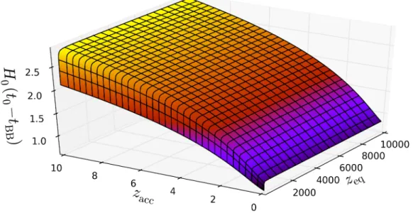
Figure 1.6.: Age of a flat universe as a function of zeq and zacc. The displayed value correspond to a numerical integration of Eq. (1.43).

With the values of Ω(0)_i recalled in table 1.2, one obtains zeq ' 3402. Here, the subscript “eq” stands for “equality” between matter and radiation. When a < aeq (or equivalently z > zeq), the Universe is dominated by radiation, ⇢tot / a−4 and a/ t1/2.

To conclude, the Universe history is made of three main phases: a radiation era for z > zeq during which ⇢tot/ 1/a4 and a/ t1/2, a matter era for zacc< z < zeq during which ⇢tot / 1/a3 and a _{/ t}2/3_{, and a dark energy era for z < z}

acc during which ⇢tot ' constant and a / eHt. These three eras can clearly be seen on the left panel of Fig. 1.5. In this discussion, the role played by curvature has not been included. Indeed, since ⇢K decays slower than, say, ⇢mat, ⇢(0)_K _{⌧ ⇢}(0)_mat implies that this inequality holds at any previous time, and curvature can never have dominated the Universe content. This is why in Fig.1.5and in this section1.3, we consider a flat universe for which Ω(0)_K = 0.

1.3.2. Age of the Universe

When the Universe is dominated by an ideal fluid, the a(t) profile has been derived in Eq. (1.30). Neglecting the transition phases between the three above mentioned eras (during which there are two equally important main constituents), we can therefore derive an approximated piece-wise form for a(t) spanning the whole Universe history. The integration constants ⇢in and tin appearing in Eq. (1.30) can be set by requiring continuity of a and ˙a at the transition times (so

(34)

1.3. The History of the Universe: the Hot Big Bang Model that H is continuous), and one obtains

a(t) a0 ' 8 > > > > < > > > > : exp [H0(t− t0)] if t > tacc 1 1+zacc ⇥1 + 3 2H0(t− tacc) ⇤2/3 if teq< t < tacc 1 1+zeq  1 + 2⇣1+zeq 1+zacc ⌘3/2 H0(t− teq) $1/2 if tBB< t < teq . (1.38)

Here, tacc is the transition time between the matter era and the dark energy era and teq is the transition time between the radiation era and the matter era. They are such that

H0(t0− tacc) = ln (1 + zacc) , (1.39) H0(tacc− teq) = 2 3 − 2 3 ✓ 1 + zacc 1 + zeq ◆3/2 . (1.40)

The piecewise function a(t) defined by Eq. (1.38) is displayed in the right panel of Fig. 1.5

(coloured lines, each colour corresponds to a different era). It is interesting to notice that when moving backwards in time, a goes to 0 in a finite amount of time. The corresponding singularity is called the Big Bang. Looking at Eq. (1.38), it occurs at the time tBB given by

t0− tBB' H₀−1 " 2 3 + ln (1 + zacc)− 1 6 ✓ 1 + zacc 1 + zeq ◆3/2# . (1.41)

One can see that as mentioned in section 1.1.1, the age of the Universe is of the order of the Hubble time H₀−1. More precisely, with the values given in table 1.2, one obtains t0 − tBB ' 0.92H₀−1 _{' 1.33 ⇥ 10}10 _year.

Obviously, the Friedmann equation (1.28) can also be solved exactly, that is the integral

t_{− t}0= H0−1 Z a/a0 1 d (˜a/a0) r P iΩ (0) i ⇣ ˜ a a0 ⌘−1−3wi (1.42)

can be computed numerically. The result is displayed with the black line in the right panel of Fig. 1.5. The matching with the piecewise approximation is fairly good. With the parameter values recalled in table1.2, this leads to a slightly different value for the age of the Universe, that is t0− tBB ' 0.95H0−1 ' 1.37 ⇥ 1010 year. Actually, since the approximated expression (1.41) for the age of the Universe is given in terms of zeq and zacc, it can be useful to express the integral (1.42) in terms of these two variables only. One obtains for the age of the Universe

t0− tBB = H₀−1 s 1 + 1 1 + zeq + (1 + zacc)3⇥ Z 1 0 dz  (1 + z)5+ 1 1 + zeq (1 + z)6+ (1 + zacc)3(1 + z)2 $−1/2 . (1.43)

One can numerically check that Eqs. (1.41) and (1.43) give similar results as soon as zeq > zacc, and that the age of the Universe increases only mildly with zeq, and more notably with zacc. The integral (1.43) is displayed in Fig.1.6as a function of zeq and zacc.

(35)

Figure 1.7.: Main events in the Cosmological Standard Scenario.

1.3.3. A Brief Cosmological History

The cosmological redshift (1.8) gives a rule for the behaviour of a black-body spectrum of radiation with temperature Tγ. Indeed, since all photons redshift as exactly the same rate λ_{/ a}−1, a system which starts out as a black-body stays as a black-body, with a temperature that decreases with expansion,

Tγ/ a−1. (1.44)

Therefore, when one goes backwards in time during the radiation era, temperature increases as 1/a. In particular, this means that the initial singularity is also a point of infinite temperature. This leads us to the standard hot Big Bang picture of the Universe: a cosmological singularity at finite time in the past, followed by a hot, radiation dominated expansion, during which the Universe gradually cools down as T _{/ a}−1 and the radiation dilutes, followed by a period of matter dominated expansion during which galaxies, stars and planets form. Finally, the vacuum energy inevitably dominates and the Universe enters a state of exponential expansion.

This simple picture allows us to infer the presence of a few notable events that we now briefly recap, and that are summarized in Fig. 1.7 with orders of magnitude about time, energy and temperature at which these events occur. As one goes backwards in time, one can check that energy or temperature increases.

Inflation takes place at t. 10−35s and is the object of section1.4and chapter2(in this section, times are given as elapsed since the initial singularity). This is why we start out our description afterwards, when the Universe is made of a hot plasma containing the fundamental particles of the standard model, at t⇠ 10−35 _s.

At t_{⇠ 10}−11s occurs the electroweak phase transition which breaks the SU (2)_{⇥U(1) symmetry} of the electroweak field into the U (1) symmetry of the present day electromagnetic field [43, 44, 45, 46, 47, 48, 49]. This transition may be important to understanding the asymmetry between the amount of matter and antimatter in the present Universe through a process of baryogenesis [50,51,52,53,54]. It occurs at the electroweak scale which is often taken to be at the Higgs vev, around 246 GeV.

In the same manner, around t _{⇠ 10}−6 s, a phase transition (associated with chiral symmetry breaking) occurs that converts a plasma of free quarks and gluons into hadrons [55,56,57,58, 59,60]. This quark-hadron transition may play an important role in the generation of primordial magnetic fields [61]. It may also give rise to important baryon number inhomogeneities which can affect the distribution of light element abundances from primordial Big Bang nucleosynthesis [62] (see below). It occurs when the temperature drops below the rest energy of nucleons, around 938 MeV.

(36)

1.3. The History of the Universe: the Hot Big Bang Model

Figure 1.8.: Big Bang Nucleosynthesis. Light elements abundances (relative to hydrogen) as a function of the density of ordinary matter Ωb and of its density relative to photons Ωb/Ωrad at time of nucleosynthesis. The WMAP satellite has been able to directly measure this ordinary matter density and found a value [63] of 4.6%(±0.2%), in-dicated by the vertical red line. This leads to predicted abundances shown by the circles in the graph, which are in good agreement with observed abundances. Image Credit: NASA/WMAP101087.

From there, nuclear fusion begins at t⇠ 0.01 s and big bang nucleosynthesis proceeds at t ⇠ 3 min. This phase is when light elements (mostly H, D, He, Li and Be) are formed [64,65,66,67]. Reproducing the observed abundances of elements from nuclear physics calculations places tight constraints on the environment it took place in [68, 69, 70, 71, 72, 73, 74, 75]. For example, in Fig. 1.8 are displayed the abundances of early produced light elements as a function of the density of ordinary matter relative to photons, Ωb/Ωrad. One can see that measures of elements abundances allow to set tight constraints on this ratio, and conversely. Nucleosynthesis begins at temperatures of around 10 MeV (which is the order of magnitude of nuclear binding energies) and ends at temperatures below 100 keV. The corresponding time interval is from a few tenths of a second to up to 103 seconds. Heavier elements are only formed later through stellar nucleosynthesis in evolving and exploding stars.

The Universe keeps on cooling down, until it reaches the point where charged electrons and protons become bound to form electrically neutral hydrogen atoms. This phase is often called “recombination” (although nuclei and electrons have never combined before). Since the photon-atom cross section (the Rayleigh section) is much smaller than the photon-electron cross-section (Thomson cross-cross-section), the Universe becomes transparent shortly after when photons decouple from matter (photon decoupling) and travel freely in the Universe. The associated

(37)

Figure 1.9.: Cosmic Microwave Background temperature fluctuations, as seen by the Planck satellite [76]. Colours encode temperature deviations from the mean temperature (blue points are colder whereas red points are hotter). Image Credit: Planck Collaboration.

relic radiation is called cosmic microwave background (CMB) and is the oldest photograph of the Universe one can get [77]. Its emission occurs at energies around 1 eV, at t ⇠500,000 y. It reaches us today with the same shape of temperature distribution, i.e. a perfect black-body spectrum, with its central temperature redshifted by the amount of expansion O"103_{# that has} occurred since then, to reach the average value TCMB= 2.725 K. This temperature is the same for all direction in the sky, up to tiny fluctuations of the order 10−5. This tells us that at recombination time, the Universe is homogeneous and isotropic on all scales up to the present horizon (see section 1.4.1) to at least one part in 100,000. The statistics of the deviations from homogeneity of this radiation is a key prediction of the theory of inflation that we discuss in chapter 2. For illustrative purpose, the spatial map of the CMB temperature fluctuations measured by the Planck satellite is displayed in Fig.1.9.

Galaxies then start to form, and inside them objects energetic enough to ionize neutral hydrogen. This is the so-called reionization epoch [78,79,80,81]. As these objects form and radiate energy, the Universe indeed goes from being neutral back to being an ionized plasma, between 150 million and one billion years after the Big Bang. Compared with before recombination however, matter is much more diluted because of the expansion of the Universe, and scattering interactions are much less frequent than at this time. This is why the subsequent Universe, full of low density ionized hydrogen, remains transparent, as is the case today.

At t _{⇠ 9 billion years, dark energy starts to dominate and the expansion accelerates [}84, 85]. First stellar systems form, and large scale structures continue to develop until today. Large scale structures constitute another observational pillar of modern cosmology, since the way they develop is related to the content of the Universe, the physical nature of its dark sector, the underlying theory of gravitation, and the initial cosmological perturbations they start from. For example, in Fig.1.10is displayed the result of simulated dark matter distributions for different cosmological models. The left panel is when structures develop in the standard cosmology described so far, the middle panel is when no dark energy is introduced in the model (Ωde= 0), and the right panel is when warm dark matter (i.e. such that wde > 0) is used instead of cold dark matter. One can see that the features of the structures are different. For example, when no dark energy is present, the Universe expansion does not accelerate at late times, which allows faster structure formation. In this manner, measuring the distribution of matter around us