HAL Id: hal-00317867
https://hal.archives-ouvertes.fr/hal-00317867
Submitted on 13 Oct 2005
HAL is a multi-disciplinary open access
archive for the deposit and dissemination of
sci-entific research documents, whether they are
pub-lished or not. The documents may come from
teaching and research institutions in France or
abroad, or from public or private research centers.
L’archive ouverte pluridisciplinaire HAL, est
destinée au dépôt et à la diffusion de documents
scientifiques de niveau recherche, publiés ou non,
émanant des établissements d’enseignement et de
recherche français ou étrangers, des laboratoires
publics ou privés.
structures associated with sporadic-E layers and QP
radar echoes
R. Pfaff, H. Freudenreich, T. Yokoyama, M. Yamamoto, S. Fukao, H. Mori, S.
Ohtsuki, N. Iwagami
To cite this version:
R. Pfaff, H. Freudenreich, T. Yokoyama, M. Yamamoto, S. Fukao, et al.. Electric field measurements
of DC and long wavelength structures associated with sporadic-E layers and QP radar echoes. Annales
Geophysicae, European Geosciences Union, 2005, 23 (7), pp.2319-2334. �hal-00317867�
SRef-ID: 1432-0576/ag/2005-23-2319 © European Geosciences Union 2005
Annales
Geophysicae
Electric field measurements of DC and long wavelength structures
associated with sporadic-E layers and QP radar echoes
R. Pfaff1, H. Freudenreich1, T. Yokoyama2, M. Yamamoto2, S. Fukao2, H. Mori3, S. Ohtsuki4, and N. Iwagami4
1NASA/Goddard Space Flight Center, Greenbelt, MD, USA
2Research Institute for Sustainable Humanosphere, Kyoto University, Kyoto, Japan
3National Institute of Information and Communications, Tokyo, Japan
4Department of Earth and Planetary Science, University of Tokyo, Tokyo, Japan
Received: 5 April 2005 – Revised: 14 July 2005 – Accepted: 7 August 2005 – Published: 13 October 2005 Part of Special Issue “SEEK-2 (Sporadic-E Experiment over Kyushu 2)”
Abstract. Electric field and plasma density data gathered on a sounding rocket launched from Uchinoura Space Cen-ter, Japan, reveal a complex electrodynamics associated with sporadic-E layers and simultaneous observations of quasi-periodic radar echoes. The electrodynamics are character-ized by spatial and temporal variations that differed consid-erably between the rocket’s upleg and downleg traversals of the lower ionosphere. Within the main sporadic-E layer (95– 110 km) on the upleg, the electric fields were variable, with amplitudes of 2–4 mV/m that changed considerably within altitude intervals of 1–3 km. The identification of polariza-tion electric fields coinciding with plasma density enhance-ments and/or depletions is not readily apparent. Within this region on the downleg, however, the direction of the electric field revealed a marked change that coincided precisely with the peak of a single, narrow sporadic-E plasma density layer near 102.5 km. This shear was presumably associated with the neutral wind shear responsible for the layer formation. The electric field data above the sporadic-E layer on the up-leg, from 110 km to the rocket apogee of 152 km, revealed a continuous train of distinct, large scale, quasi-periodic structures with wavelengths of 10–15 km and wavevectors oriented between the NE-SW quadrants. The electric field structures had typical amplitudes of 3–5 mV/m with one ex-cursion to 9 mV/m, and in a very general sense, were asso-ciated with perturbations in the plasma density. The elec-tric field waveforms showed evidence for steepening and/or convergence effects and presumably had mapped upwards along the magnetic field from the sporadic-E region below. Candidate mechanisms to explain the origin of these
struc-tures include the Kelvin-Helmholtz instability and the Es
-layer instability. In both cases, the same shear that formed the sporadic-E layer would provide the energy to generate
Correspondence to: R. Pfaff
the km-scale structures. Other possibilities include gravity waves or a combination of these processes. The data sug-gest that these structures were associated with the lower al-titude density striations that were the seat of the QP radar echoes observed simultaneously. They also appear to have been associated with the mechanism responsible for a well-defined pattern of “whorls” in the neutral wind data that were revealed in a chemical trail released by a second sounding rocket launched 15 min later. Short scale (<100 m) electric field irregularities were also observed and were strongest in the sporadic-E region below 110 km. The irregularities were organized into 2–3 layers on the upleg, where the plasma density also displayed multiple layers, yet were confined to a single layer on the downleg where the plasma density showed a single, well-defined sporadic-E peak. The linear gradient drift instability involving the DC electric field and the verti-cal plasma gradient is shown to be incapable of driving the observed waves on the upleg, but may have contributed to the growth of short scale waves on the topside of the narrow unstable density gradient observed on the downleg. The data suggest that other sources of free energy may have been im-portant factors for the growth of the short scale irregularities.
Keywords. Ionosphere (Mid-latitude ionosphere; Electric fields and currents; Ionospheric irregularities)
1 Introduction
The “Sporadic-E Experiment over Kyushu” (SEEK) ex-periments combine in-situ and ground-based measurements in order to advance our understanding of the electrody-namic properties and neutral wind forcing of the mid-latitude lower ionosphere during sporadic-E conditions when quasi-periodic radar echoes are present. The SEEK-1 campaign
Position at 105 km altitude: upleg downleg 131¡E 130¡E 132¡E S-310-31 Trajectory S-310-32 Trajectory 133¡E 134¡E 30¡N 32¡N 33¡N 31¡N JA PA N Uchinoura Space Center Tanegashima (South) Radar Kochi Radar line-of-sight Scattering region P A C I F I C O C E A N 0 50 (km) 100 B G eo g rap h ic L at it ud e Geographic Longitude
Fig. 1. Horizontal projection of the trajectories of the SEEK-2
sounding rockets and the Tanegashima south radar beam.
(Fukao et al., 1998) was conducted in August, 1996 from the Uchinoura Space Center located to the south of Kyushu Island, Japan. This joint rocket, radar, and ground-based investigation returned a wealth of information concerning sporadic-E phenomena and QP echoes including evidence for large wind shears (Larsen et al., 1998), localized polar-ization electric fields within and above the sporadic-E layers (Pfaff et al., 1998), and the existence of broad spectra of ir-regularities in both the electric field and plasma density data (Pfaff et al., 1998; Mori and Oyama, 1998).
The SEEK-2 campaign was carried out in August 2002, from the same location. Although the general investigation was similar to that of SEEK-1, several important changes
were made. Besides the addition of more
comprehen-sive ground-based measurements and the inclusion of to-mographic radio beacons to determine the horizontal spatial structure of the plasma density, two rockets were launched 15 min apart on the same night that included a variety of probe measurements as well as luminous trails to measure neutral winds. Both rockets were launched in the presence of QP radar echoes and sporadic-E conditions. Details of the SEEK-2 campaign and experiment objectives may be found in Yamamoto et al. (2005).
In this paper, we present detailed electric field double probe measurements gathered on the first SEEK-2 sounding rocket (S310-31). We report measurements of DC electric fields and large amplitude, wavelike electric structures prop-agating in the NE-SW quadrants. We relate the electric field measurements to simultaneous measurements of plasma den-sity as well as to the neutral wind measurements gathered on the second SEEK-2 rocket (S310-32) launched 15 min later. Finally, we report observations of short-scale electric field
irregularities gathered with the double probe detector. The observations are interpreted in terms of current theories of sporadic-E physics. They also serve as comparisons for nu-merical simulation studies presented in a companion paper (Yokoyama et al., 2005).
An outline of this paper is as follows. We first provide an overview of the electric field experiment and payload geom-etry. We then present the measurements and basic analysis of the DC and long wavelength electric fields. This is followed by comparisons with the plasma density measurements and an analysis of the shorter scale (higher frequency) measure-ments. The paper concludes with a discussion and summary.
2 Experiment overview
The data reported here were gathered on the Japanese sound-ing rocket S310-31 which was launched on 3 August 2002 at 23:24 LT from the launch range at Uchinoura, Japan. The rocket achieved an apogee of 151.9 km at 193.9 s after liftoff. The rocket trajectory was predominantly eastward and in-cluded a large horizontal velocity of 777 m/s such that the upleg and downleg traversals of the lower-E-region (105 km) were separated by about 157 km, as shown in Fig. 1. The geophysical conditions at launch are described by Yamamoto et al. (2005).
The S310-31 payload was equipped with a dual set of or-thogonal double probes of 4.0 m (tip-to-tip) length to mea-sure both DC and wave (or AC) electric fields in the spin plane of the payload, as shown in Fig. 2. This experiment was identical to the electric field experiment on the SEEK-1 rocket (Pfaff et al., SEEK-1998). Spherical sensors with 4.4 cm diameter were used to gather the potentials which were
de-tected with high impedance (>1012)pre-amplifiers using
the floating (unbiased) double probe technique. The potential differences on the two main orthogonal axes were digitized on-board using 16-bit analog-digital converters, sampled at 1600 samples/s with anti-aliasing filters at 800 Hz.
The electric field measurement coordinate system is shown in Fig. 2 in which the x and y components represent the orthogonal spin plane potential differences measured be-tween spheres 1 and 2 and spheres 3 and 4, respectively. The
zcomponent is subsequently computed on the ground based
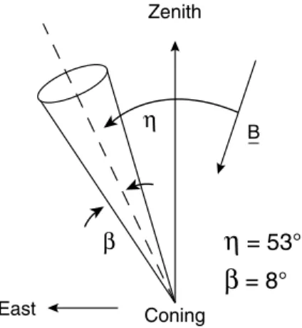
on these two measurements, as will be explained later. The payload attitude during the flight was such that the an-gle between the coning axis and the magnetic field was
cen-tered at 53◦pitched towards the east, as shown in Fig. 3. The
coning was characterized by a half angle of 8◦and a period of
243 s, and did not appear to degrade the measurements in any noticeable way. The vehicle motor casing, for which the ex-posed surface was conducting, was retained with the payload during the flight. A star sensor and magnetometer provided attitude data with an accuracy of about 1 deg.
3 Data presentation and analysis – DC electric field measurements
3.1 Overview of the raw electric field data
The principal electric field data were gathered from the two crossed (perpendicular) double probes in the rocket spin plane and are shown in the middle and lower panels of Fig. 4 for the entire flight while the payload was in the iono-sphere (>90 km). The potential differences measured
be-tween spheres 1 and 2, or Ex, are shown in the middle panel
and those potentials measured between spheres 3 and 4, or
Ey, are shown in the lower panel. As these measured fields
are in the spacecraft frame, the large sine waves result from the payload rotation at the spin period of 1.38 s. The largest contribution to the electric field measurements by double probes moving through the ionosphere at mid-latitudes is that due to the V ×B fields created by their motion across the am-bient magnetic field, where V is the rocket velocity in the Earth-fixed reference frame and B is the ambient magnetic field.
The large sine waves corresponding to Exand Eyin Fig. 4
are essentially 90 deg out of phase, as expected for orthogo-nal, spin plane DC electric field measurements on a spinning payload. (This phase shift is easier to see on expanded time scale representations, as will be shown in the next figure.) Detailed inspection of the two orthogonal measurements re-veal that they agree to within 1% with a small phase
de-parture of 1.5◦ from strict orthogonality. Adjustments for
these small amplitude and phase variations, as well as slowly changing DC offsets due to the sphere contact potentials and other sources, have been applied to the data used to compute the DC electric field solution that follows.
The sum of the squares of the two components in the lower panels are shown in the upper panel in Fig. 4 and represents the magnitude of the DC electric field in the spin plane of the payload. These data reveal abrupt, large-scale variations which can immediately be attributed to changes in the geo-physical electric field since the V ×B fields are slowly vary-ing. The sum of the squares data also reveal contributions at the spin frequency and its harmonics. These contributions result primarily from distortions of the sinuso¨ıdal waveforms in the raw data. We discuss this topic in more detail below.
3.2 Detailed examination of the measured potentials
Before calculating the geophysical DC electric fields, we per-form a detailed inspection of the raw data and the higher fre-quency contributions to the potential differences. In addition to examining the data for evidence of plasma waves and ir-regularities, we seek to identify and, if possible, remove any non-geophysical contributions to the measured potentials. Figures 5a and b show enlargements of the raw data in Fig. 4 for 13 s intervals of the flight during the upleg and downleg sporadic-E encounters corresponding to ∼97–109 km. The
Exdata are shown in the upper portion of the figures whereas
the Eydata are presented in the lower portion. The raw data
ω spin Electric Field Probes Langmuir Probe 1 2 3 4 Ez Ey Ex
ω
spin Electric Field Probes Langmuir Probe 1 2 3 4 Ez Ey ExFig. 2. Payload measurement geometry and associated coordinate
system. Zenith Coning East B
η
= 53°
β
= 8°
η
β
Fig. 3. Coning angle of the rocket with respect to the magnetic field.
have been filtered at 5 Hz and the higher frequency compo-nents are shown beneath the raw, DC-coupled waveforms.
Examination of the large amplitude spin period wave-forms reveal departures from pure sine waves for reasons that are both geophysical and non-geophysical. The geo-physical variations are due to large scale irregularities and structures associated with the sporadic-E layers that are the main subject of this paper. The upleg data in Fig. 5a shows a lower layer of irregularities between 84–89 s and an up-per layer between 93–96 s. On the other hand, the downleg data in Fig. 5b show only one layer of irregularities between
Uchinoura, Japan – – SEEK 2 (S310-31) 3 August 2002
Apogee Altitude (km)
Seconds after launch
100 110 120 130 140 150 150 140 130 120 110 100 60 60 30 0 – 30 – 60 60 30 0 – 30 – 60 40 20 0 (EX2+E Y2) 1/2 EX EY 100 150 200 250 300 mV/m mV/m mV/m
Fig. 4. Raw data from the two perpendicular, spin plane electric field detectors (lower panels). The upper panel is the magnitude of these
components.
Upleg
Uchinoura, Japan – – SEEK 2 (S310-31) 3 August 2002
Altitude (km)
Seconds after launch
98 100 102 104 106 108 40 20 0 – 20 – 40 40 20 0 – 20 – 40 mV/m mV/m mV/m mV/m 2 4 – 4 0 – 2 2 4 – 4 0 – 2 δEX, f > 5 Hz δEY, f > 5 Hz EX EY 86 84 88 90 92 94 96 (a) Downleg Altitude (km)
Seconds after launch
108 106 104 102 100 98 40 20 0 – 20 – 40 40 20 0 – 20 – 40 mV/m mV/m mV/m mV/m 2 4 – 4 0 – 2 2 4 – 4 0 – 2 δEX, f > 5 Hz δEY, f > 5 Hz EX EY 294 292 296 298 300 302 (b)
Fig. 5. (a) An expanded view of the raw electric field data gathered between 97 and 109 km on the upleg together with the filtered (wave)
data for frequencies greater than 5 Hz. (b) Same as Fig. 5a but for the downleg.
292–297 s. As can be seen in the figures, the shorter scale (i.e. filtered data) irregularities had amplitudes of approxi-mately +2–3 mV/m and were somewhat stronger during the upleg. We will return to these higher frequency irregularities later on below.
The data also include “spikes” that appear simultaneously in both waveforms that are attributed to interference from other instruments on the payload. The most prominent of these spikes have been removed from the data and thus con-stitute the brief intervals where no data are shown. In some
cases, smaller spikes were not removed and hence may con-tribute to the presence of “irregularities”. These small spikes appear more prominent in the downleg filtered data.
In order to best determine the DC electric field, we fit model sine waves at the spin frequency of 0.72 Hz to the
Ex and Ey data for the entire flight. We first identify
non-geophysical contributions to the DC electric field waveforms (e.g. from magnetic shadowing, wake, and interference ef-fects) and then compute the model fits from only those por-tions of the waveforms that are related to geophysical elec-tric fields. The sine wave fits are computed for every data
point in a progressive manner for both the Exand Ey
wave-forms. Consequently, the DC electric field data shown below are essentially low pass filtered below the spin frequency of 0.72 Hz.
3.3 DC electric field solution
Since the electric field component along the spin axis, Ez,
was not measured, vector electric fields are obtained assum-ing E·B=0, where E is the electric field vector and B is the
magnetic field vector. In this manner, we calculate what Ez
would have been based on the measured Ex and Ey data in
order to satisfy this relation. The geometry is shown in Fig. 2.
The corresponding values of Ezare shown in the center panel
of Fig. 6 based on the model fits of Ex and Ey discussed
above. The accuracy of the Ezderivation depends on the
an-gle between the spin axis and the magnetic field. Clearly, as the angle approaches 90 deg, the magnetic field vector would then lie near or within the spin plane and thus it would
be-come increasingly difficult to derive Ezusing the assumption
that there are no electric fields parallel to B. For this experi-ment, the angle between the spin axis and the magnetic field varied between 120–135 deg for the entire flight, as shown
in the top panel of Fig. 6. The Ez computations represent
the spin axis electric field component with a high degree of
confidence due to the lack of a large variation in the Ezdata
associated with the coning angle, as well as the fact that most
of the Ezpotential corresponds to the z-component of V ×B,
as shown in the middle panel of Fig. 6. Note that Ez varies
with the angle between the spin axis and the velocity vector, as shown in the top panel of Fig. 6.
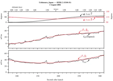
The lowest panel of Fig. 6 shows the sum of the squares of
the measured Exand Eycomponents, whose amplitudes now
correspond to those of the sine wave fits discussed above, and
the computed Ezcomponent. This sum represents the
mag-nitude of the combined ambient geophysical and V ×B elec-tric fields encountered by the payload. We have overlaid the V ×Bmagnitude based on the measured rocket velocity and the model magnetic field. Notice that most of the measured potential corresponds to the V ×Bcontribution. The depar-tures from the V ×B induced field are the geophysical fields we seek to extract, characterize, and understand.
The next step is to subtract the V ×B fields from the Ex,
Ey, and Ez components. The attitude data are then used
to rotate the fields from the payload reference frame into geophysical coordinates. The resulting fields are presented
Uchinoura, Japan Ð Ð SEEK 2 (S310-31) 3 August 2002
Apogee
Altitude (km)
Seconds after launch
100110 120 130 140 150 150 140 130 120 110100 180 90 0 100 150 200 250 300 m V/ m m V/ m de gre es 180 135 90 de gre es 40 20 0 60 40 20 0 EZ(computed) (V x B)Z ETOT Z axis, B Z axis, V | V x B |
Fig. 6. The computed spin axis electric field component, Ez, and the
corresponding V ×B component (middle panel). The total electric field and computed V ×B fields (lower panel). The upper panel shows the angle between the spin axis (z) and the velocity vector and the angle between the spin axis (z) and the magnetic field vector (see scale on right).
in zonal and meridional geomagnetic coordinates in Fig. 7 along with vector (or arrow) plots of the fields. Notice that the electric fields are characterized by large amplitude struc-tures with a quasi-periodic nature. In particular, the electric field structures display a period of roughly 20–30 s, primar-ily within the flight time period of 100–200 s, as shown in the lowest panel. Notice further that the ambient DC or static electric field is quite small. We discuss the structured fields in more detail below.
3.4 Plasma density measurements
The plasma density measurements from the fixed-bias Lang-muir probe are shown in the upper panel of Fig. 7. They have been normalized using the absolute density obtained from the impedance probe (Wakabayashi et al., 2005). On the upleg, the data reveal two main layers at 103 km and 105 km with
peak amplitudes near 105cm−3. A single, narrower layer is
observed near 102.5 km on the downleg with a peak density
of 8×104cm−3. The plasma density data show variations
throughout the flight, as discussed below.
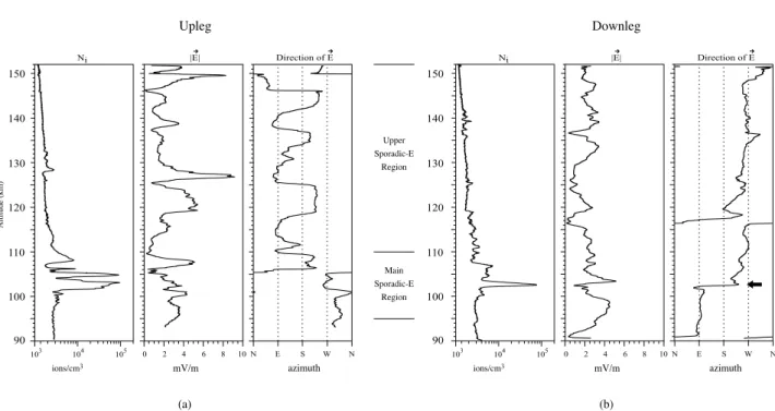
The plasma density and DC electric field results are dis-played versus altitude in Fig. 8a for the upleg and Fig. 8b for the downleg. Notice that the sporadic-E region between 95–110 km is broader and more structured in the plasma den-sity data on the upleg, which corresponds more directly to the region of QP radar echoes observed between 95–105 km during the flight (Saito et al., 2005). Above the sporadic-E layer, both the density and electric field data reveal a struc-turing at altitudes which are not the same between the up-leg and downup-leg. We interpret this structuring as that due to space/time variations encountered by the payload and not due to a layering with altitude. In other words, if the structur-ing were due to broad, stable horizontal layers, then the same
Altitude (km) 100 100 90 90 110120 130 140 150 150 140 130 120 110 mV/m mV/m cm -3 5 10 – 10 0 – 5 5 10 – 10 0 – 5 105 104 103 Ezonal Emeridional Plasma Density 150 100 200 250 300
Uchinoura, Japan – – SEEK 2 (S310-31) 3 August 2002 Apogee 4 mV/m meridonial: az, el = 354.6°, 46.2° zonal: az, el = 84.6°, 0.0° N E B in
Seconds after launch
North
South East
West
Fig. 7. The DC electric field solution in magnetic coordinates with the plasma density shown in the uppermost panel.
altitudes would be affected on both the upleg and downleg, as also discussed in Kelley et al. (1995).
3.5 Large amplitude periodic structures
We proceed by interpreting the large scale variations in the electric field and plasma density above about 107 km on the upleg as signatures of large amplitude, quasi-periodic struc-tures. The quasi-periodic variations in the electric field data, particularly in azimuth, reveal a characteristic spacing of
∼20–30 s as shown in the middle and lower panels of Fig. 9.
This period was also readily apparent in the electric field ar-row plots in the lowest panel of Fig. 7. The upper panel of Fig. 9 shows the plasma density variations versus time in a 1N/N format. Here, we compute a smoothed “ambient” plasma density based on average values of the density. We then compute the ratio: (raw data – ambient)/ambient to
cre-ate the 1N/N signature. There is a general structure in the 1N/N data that suggests a relationship with the electric field structure. However, there is no apparent, detailed correspon-dence between the 1N/N and 1E amplitudes. We now seek to characterize the temporal periodic structure observed in the vector electric field data as a wavevector.
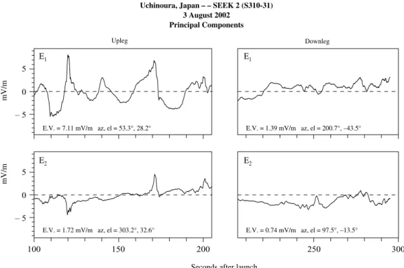
In order to obtain a more definitive measure of the wavevector direction and period associated with the elec-tric field quasi-periodic structures, we perform a minimum variance analysis. This provides the principal component of the electric field structures. We restrict ourselves to the data above the sporadic-E layer (i.e. >110 km) and separate the upleg and downleg portions of the flight. The results are shown in Fig. 10. The direction of the principal component
for the upleg data is 53.3◦(or northeast) and 200.7◦(or
south-west) for the downleg data. There is a 180 deg ambiguity in each of these measurements. The eigenvalue ratio between
Altit ude ( km ) 90 100 120 110 130 140 150 90 100 120 110 130 140 150 Uchinoura, Japan Ð Ð SEEK 2 (S310-31)
3 August 2002 Upleg Downleg 8 6 4 2 0 10 mV/m ions/cm3 Ni 105 104 103 |E| S E N W N azimuth Direction of E 8 6 4 2 0 10 mV/m (b) (a) ions/cm3 Upper Sporadic-E Region Main Sporadic-E Region Ni 105 104 103 |E| S E N W N azimuth Direction of E
Fig. 8. Electric field and plasma density displayed versus altitude for the upleg (a) and downleg (b).
QuasiÐPeriodic Structure Altitude (km) 100 110 120 130 140 150 150 140 130 120 110 100 90 m V/ m de g re e s % 0 20 6 Ð 20 8 2 4 0 0 90 180 360 270 80 100 60 40 azimuth of E magnitude of E ∆Ni/Ni 150 100 200 250 300
Uchinoura, Japan Ð Ð SEEK 2 (S310-31) 3 August 2002
Seconds after launch
North
North
South East West
Uchinoura, Japan – – SEEK 2 (S310-31) 3 August 2002
Principal Components
Seconds after launch
100 150 200 250 300 mV/m mV/m – 5 5 0 – 5 5 0 E2 E1 E2 E1 E.V. = 7.11 mV/m az, el = 53.3°, 28.2° Upleg Downleg E.V. = 1.39 mV/m az, el = 200.7°, –43.5°
E.V. = 1.72 mV/m az, el = 303.2°, 32.6° E.V. = 0.74 mV/m az, el = 97.5°, –13.5°
Fig. 10. Minimum variance solution for the upleg (left) and downleg (right) electric field structures above the sporadic-E layer (>110 km).
The solution provides the principal component (E1)and secondary component (E2). The eigenvalues (E.V.) are noted in the lower left of the panels as well as the azimuth and elevation of each component.
the principal and secondary components is much stronger for the upleg data (4.1) than for the downleg data (1.9) indicating that the variations are much more well-defined in this region on the upleg. Accordingly, we concentrate on these data in our analysis.
Notice that the electric field variations on the upleg are not sinusoidal but reveal steepened structures, similar in some ways to the narrow plasma density variations shown in Fig. 9. Further, notice in the upleg data in Fig. 10 that, although most of the variations are in the direction of the principal component as expected, the secondary component does show electric field variations in opposite directions at 50 s intervals corresponding to those times when the electric field was par-ticularly strong. The significance of this is not clear. Such features are difficult to fully ascertain because the data inter-val is limited by the relatively brief rocket trajectory.
The upleg variations display a characteristic periodicity of
20–30 s. We can relate the rocket velocity, Vr, wavevector,
k, observed frequency, ω, and the phase velocity, Vφ, by the
Doppler shift relation:
ω=k·Vr+kVφ
Since the rocket velocity along the principal component was 434 m/s, the wavelength estimate is 9–13 km, if the phase velocity is 0 m/s. If the intrinsic wave velocity were 50 m/s towards the southwest, as suggested by the QP echo time lag observed between the two radars (Saito et al., 2005), the wavelength is estimated to be 10–15 km. The vector relations are shown in Fig. 11. In the discussion section, we will relate
the wavelength and velocity direction to those observed by the QP radar data as well as with theoretical considerations.
3.6 Wave electric field measurements
Shorter-scale or higher frequency plasma waves were de-tected by the same detectors that gathered the DC electric field data. Figure 12 displays spectrograms (plotted vs.
al-titude) of the wave power detected by the Ex double probe
for the upleg and downleg. The spectrograms represent the power spectral density of the waves computed using the Fourier transform with Hanning windows for which the time-ordered spectra were subsequently mapped into equal alti-tude bins. The plasma density data are also plotted for refer-ence. The higher frequency waves in the lower-E region (95– 110 km) are the shorter-scale irregularities associated with the sporadic-E layer that were also shown in Figs. 5a and b. Notice that there is also some evidence for smaller am-plitude, narrow layers of low frequency plasma waves asso-ciated with the large scale density structures at higher alti-tudes, for example at 117 km, 127 km, and 150 km on the upleg. The downleg spectrogram shows evidence of a some-what continuous, though patchy, ensemble of very low fre-quency (<20 Hz) waves within the upper sporadic-E region between 108–142 km, in likely association with the highly structured plasma density within this region. As is clear in the spectrograms, however, the strongest and the broadest irregularity signatures are confined to the main sporadic-E regions below 110 km.
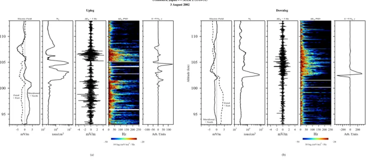
Figure 13 provides enlargements of the sporadic-E re-gion from 93–113 km for the upleg (a) and downleg
(b). Here are shown the DC electric field, plasma
den-sity, electric field waveform (Ex) filtered above 5 Hz, the
corresponding electric field spectrogram from 0–250 Hz, and the product of the vertical component of the DC electric field and the vertical density gradient. This last parameter is im-portant for growth rate considerations and will be discussed further on below. White lines in the sonograms correspond to large gaps in the data where non-geophysical signals were re-moved. Smaller gaps in the data did not result in white lines in the spectrograms as interpolation techniques between ad-jacent spectra were employed.
With respect to the interpretation of the wave electric field data, we note that it is difficult to relate wave frequency to wavelength without knowledge of the wavevector direction and phase velocity (e.g. Fredricks and Coroniti, 1976). As the horizontal component of the rocket velocity was 777 m/s, a 10 m wave in this direction with a small phase velocity (i.e.
Vφ Vr)would thus appear in the payload reference frame
at 77 Hz. A horizontal 10 m wave with near-zero phase
ve-locity traveling at 45◦to the rocket velocity would appear at
55 Hz in the rocket frame. Although higher frequencies nor-mally correspond to shorter scales, the converse is not nec-essarily true, since short scale waves oriented at directions oblique to the rocket velocity contribute to wave power at lower frequencies.
The power spectral densities shown in these spectrograms include some modulation at twice the rocket spin period, which is revealed to some extent in the filtered time se-ries data shown earlier in Figs. 5a and b. Such modulation from data gathered with a spinning electric field detector may sometimes be used to determine the direction of the observed electrostatic waves, since k is parallel to δE for electrostatic waves. However, due to their brief encounters by the rocket probes and the interference present in the raw data, the direc-tion of the short scale waves is difficult to discern. Detailed analysis (not shown) of the irregularities reveals that their di-rections appear somewhat isotropic (at least within the spin plane) on the upleg, whereas the downleg data display a more distinct twice-per-spin modulation (see in particular the
fil-tered Ey data in Fig. 5b), indicative that these wavevectors
are predominantly organized in one direction.
4 Discussion
The electric field and plasma density data reveal a com-plex electrodynamics associated with the sporadic-E layer and nearby QP radar echo region observed during the rocket flight. We now discuss the observations and attempt to re-late them to physical processes operating in the earth’s lower ionosphere during this event. Our approach is to organize the observations into two different regions: the main sporadic-E region (95–110 km) and the upper sporadic-E region (110– 152 km). We seek to understand the phenomena distinct to
53° 5° North East Magnetic East kprincipal Vrocket
Fig. 11. The principal component of the observed, large scale
elec-tric field wavevector for the upleg with respect to the horizontal rocket velocity and the horizontal magnetic field coordinates.
each region, as well as to understand how the two regions interact.
4.1 Ambient “background” DC electric fields
The ambient or background ionosphere DC electric fields encountered by this rocket on the upleg are difficult to dis-cern due to the highly variable electric fields present within and above the sporadic-E layer. The downleg data above the sporadic-E region (i.e. 110–152 km) were not charac-terized by such large amplitude structure and revealed am-bient ionospheric DC electric fields of ∼2 mV/m that were generally in the westward direction. For these data gathered at mid-latitudes near midnight, the amplitude and direction of this field agrees with MU radar observations in Japan for the same local time and season (Oliver et al, 1993). The con-tribution to the lower ionosphere electric field set up by local neutral winds and plasma density layers compared to global electric fields that mapped down along the magnetic field from the ionosphere above is not immediately clear. Nev-ertheless, this ambient ionospheric DC electric field might have contributed as a driver of the large scale dynamics rel-evant to the physics of the sporadic-E layer discussed here. Such fields are also important when evaluating the E and F region coupling during sporadic-E events.
4.2 Polarization electric fields
Polarization DC electric fields within the main sporadic E region (95–110 km) may be set up by a variety of processes that are complex and arise from a variety of sources. These include:
1. Direct generation via differential ion-electron drag driven by the neutral wind,
2. Static fields set up by charge separation within and be-tween layers including enhanced Cowling conductivity
Uchinoura, Japan Ð Ð SEEK 2 (S310-31) 3 August 2002 Upleg Downleg 200 150 100 50 0 250 Hz ions/cm3 Ni ∆Ex 105 104 103 A lti tu d e ( k m) 10 lo g ( m V/ m ) 2 / Hz 90 100 120 110 130 140 150 Ð50 Ð20 200 150 100 50 0 250 Hz ions/cm3 Ni ∆Ex 105 104 103 10 lo g ( m V/ m ) 2 / Hz 90 100 120 110 130 140 150 Ð50 Ð20 (b) (a)
Fig. 12. Spectrograms of the filtered Exdata (right hand panels) plotted alongside the plasma density data (left hand panels) for the upleg
(a) and downleg (b).
enhancements in regions of finite horizontal width as suggested by Haldoupis et al. (1996), and
3. Fields associated with large scale motions of the layer and instabilities.
Although it is difficult to sort out these processes definitively, particularly without a simultaneous, local measurement of the neutral wind (i.e. on the same payload), we comment on the different processes that the observations suggest may be at work in the sporadic-E layer.
The DC electric field observed in the main sporadic-E region (95–110 km) exhibited typical amplitudes of ∼2– 4 mV/m as shown in Figs. 13a and b. Although the elec-tric fields include variability in amplitude and direction, no consistent correlation between these variations and those of the plasma density layers were readily apparent, with a few
exceptions noted below. For example, on the upleg
be-tween 102–105 km, the plasma density is divided bebe-tween
two peaks with amplitudes near 105cm−3and altitude
thick-nesses of 1–2 km. Between the density peaks, a “valley” with an altitude extent of about 1 km exists at 104 km in which the
density dips to 3×103cm−3. However, throughout this
inter-val, the DC electric field does not exhibit much variation in amplitude or direction, despite the fact that the Hall mobility peaks near 105 km. Further, there is no enhancement of the zonal electric field due to the finite zonal horizontal extent of the layer that would produce an enhanced localized Cowling conductivity, as proposed by Haldoupis et al. (1996). In the sporadic-E region on the upleg from 90 km to 110 km, there
is a general trend for the direction of the electric field to ro-tate from west through south to the east, as shown in Fig. 8a. Perhaps this changing direction is related to the general wind pattern, although it is not presently understood.
Within the 1–2 km altitude interval near 107 km, the upleg data do show a marked ∼5 mV/m enhancement of the DC electric field amplitude (see Fig. 8a) that corresponds to some extent to the simultaneous depletion of the electron density, although the peak electric field is about 1 km above the alti-tude where the depletion has its lowest value. This signature is somewhat similar to the sharp 20 mV/m polarization elec-tric field enhancement observed near 122 km on the upleg of the SEEK-1 rocket (Pfaff et al., 1998), although not nearly as intense or as distinct. The azimuth of the electric field changes abruptly near 105.5 km on the upleg, as the electric field varies through zero, suggesting the presence of a shear node. (Of course, the direction of the electric field is difficult to determine when its amplitude is near zero, as seen in other instances in the data in Figs. 8a and b when the electric field amplitude becomes very small.) Indeed, the 5 mV/m peak at 107 km is in the southwest direction and may be evidence of the lowest altitude where the quasi-periodic structuring dis-cussed in the next section “emerges” from the sporadic-E region and becomes distinct.
The most striking evidence for a DC electric field signa-ture in the sporadic-E region that corresponds to a variation in the plasma density is that shown in the downleg data near 102.5 km. Here, a strong change in the DC electric field di-rection is coincident with the isolated, narrow sporadic-E
Upleg Altitude (km) 5 -5 0 -4 -2 0 2 4 0 50 100 150 200 250 -100 -50 0 50100 95 100 105 110 Hz mV/m
ions/cm3 Arb. Units
mV/m 105 104 103 Ni ∆Ex > 5 Hz ∆Ex PSD Electric Field Zonal + East Meridional + North (a) –50 –20 10 log (mV/m)2 / Hz E • Ni, z∆ Hz –50 –20 10 log (mV/m)2 / Hz Downleg Uchinoura, Japan – – SEEK 2 (S310-31)
3 August 2002 Altitude (km) 5 -5 0 -4 -2 0 2 4 0 50 100 150 200250 -200 0 200 95 100 105 110 mV/m
ions/cm3 Arb. Units
mV/m 105 104 103 Ni ∆Ex > 5 Hz ∆Ex PSD Electric Field Zonal + East Meridional + North (b) E • Ni, z∆
Fig. 13. (a) Expanded view of the upleg measurements in the sporadic-E region (93–113 km). The panels show (from left to right) the DC
electric field, plasma density, 1Exwaveform for frequencies >5 Hz, 1Exspectrogram, and the scalar product of the DC electric field and
the vertical gradient of the plasma number density. (b) Same as Fig. 13a but for the downleg.
plasma density peak of 8×104cm−3. Both the zonal and
meridional electric field components increase to some ex-tent just above and just below the layer (see Fig. 13b), while rotating through zero where the layer density peaks (see ar-row in Fig. 8b). This pronounced variation in the DC electric field presumably corresponds to the assumed neutral wind shear responsible for the layer. The mechanism that created this change in the zonal electric field is not clear, since the U ×B equivalent electric field would only be observed in a reference frame moving with the neutral wind (U), and would furthermore be expected in the meridional component for a classic sporadic-E layer set up by a zonal wind shear (e.g. Whitehead, 1970). If the sporadic-E layer contains zonal density gradients, then a zonal neutral wind could generate zonal polarization electric fields via the “Hall polarization” process discussed by Tsunoda et al. (2004).
The electric field shear at the sporadic-E peak on the downleg is also interesting because the “ambient” DC elec-tric field appears to change direction above and below the layer and not just in the few km altitude region defined by the layer. In other words, below the layer, the predominate DC electric field is eastward, yet it is westward above the layer, as discussed above in the ambient DC electric field section. These very low altitude (<100 km) electric fields suggest a strong dependence on the local neutral winds implying that they may dominate the global ionospheric DC electric fields that map down from above.
The correspondence of the large scale electric field and plasma density variations in the SEEK-2 data suggest a com-plex relationship between these quantities, including shifts between the electric field and density waveforms that may be due to dynamics that can not be fully captured by a snapshot
of measurements along a one-dimensional rocket trajectory. Further, this relationship would be expected to be a non-local one, in which the DC electric field maps along the field line and would more likely be correlated with the integrated den-sity along the magnetic field line rather than with the locally measured density. Multiple plasma density layers such as those observed within the upleg sporadic-E region may, in fact, be more appropriately considered as time-varying enti-ties, resulting from large scale instabilities (discussed below) and for which a “steady-state” picture is inadequate to ex-plain the observations.
4.3 Large scale structure
Pronounced, large scale variations in the electric field data were observed in the upper sporadic-E region (110–152 km) during the upleg, as shown in particular in Figs. 7, 8, and 9. It is clear from the data that these variations are organized with respect to time and not altitude. The periodic variations are considerably longer than the spin period of the rocket, are far shorter than the coning period, and are almost certainly of geophysical origin.
A summary of the main features of the periodic structures observed in the rocket data above 110 km are as follows:
1. The electric field data reveal a well-defined, quasi-periodic structuring above the sporadic-E layer that is continuous from 110 km to the rocket apogee of 152 km. 2. The dominant rocket frame period varies from 20–30 s. 3. Typical electric field amplitudes are 3–5 mV/m, with
S310-31 Launch
S310-32 Launch 32 MHz Backscatter Radar – – Tanegashima, Japan
3 August 2002
~13–15 km spacing
Fig. 14. Range-time-intensity plot of 32 MHz radar echoes from Tanegashima (south) showing QP echo structure (Saito et al., 2005).
4. A minimum variance analysis shows that the wavefronts are oriented in the NE-SW quadrants, along an azimuth
that is oriented 53◦east of geographic north.
5. The rocket frame period corresponds to wavelengths of 10–15 km assuming a phase velocity of 50 m/s towards the southwest.
6. The electric field waveforms are not sinusoidal, but show evidence of steepening and possible convergence at the source.
7. There is a coarse structuring in the plasma density data with typical 1N/N amplitudes of 10–20% that displays a general correspondence to the electric field structure. However, there is no consistent, detailed relationship between the 1E and 1N/N amplitudes for these struc-tures, even though the largest electric field structure am-plitude (9 mV/m) was observed in conjunction with the largest 1N/N value (∼50%).
8. Some of the electric field structures have associated bursts of weak, shorter-scale electric field irregularities, for example, at 127.5 km and at 150 km.
9. The downleg data show much weaker (1–2 mV/m), km-scale electric field structures that were also oriented in the NE/SW quadrants, though did not show a distinct period. On the other hand, the downleg data reveal a more structured plasma density profile.
We now seek to understand the processes responsible for these structures, as well as their relation to both the simul-taneous observations of QP radar echoes and the variations in the neutral wind revealed in a chemical trail released by a second rocket launched 15 min later.
The quasi-periodic (QP) echoes observed by the 32 MHz Tanegashima coherent scatter radar during this flight are shown in Fig. 14 (Saito et al., 2005). These authors com-pare data from two spatially separated radars from which it is concluded that the QP echo structures appear to be travel-ing at approximately 50 m/s from the northeast to the south-west. Based on this velocity, the QP echo striations observed during the launch and shown in Fig. 14 have spacings of
∼13–15 km around the time of the launch. These scales
are very similar to those of the dominant electric field and plasma density structures observed in the upleg in-situ mea-surements presented here.
The prime candidate mechanisms to explain these large scale structures include:
1. The Kelvin Helmholtz instability,
2. The Es-layer or Azimuth-Dependent instability, and
3. Gravity waves.
We now briefly discuss each mechanism in the context of the observations.
Kelvin-Helmholtz instability: The Kelvin-Helmholtz
instability (KHI) results from the same shear in the neutral wind that sets up the sporadic-E layer. A velocity shear associated with two layers of different density may become unstable, generating a series of “whorls” or billows whose wavelength depends on the thickness of the layer (e.g. Drazin and Reid, 1981). The instability thus creates a series of patches of density and velocity that evolve to increasingly smaller spatial scales with time. KHI has been proposed by Larsen (2000) as a possible explanation for QP radar echoes, arguing that the neutral winds associated with numerous sporadic-E events are sufficiently unstable (i.e.
Uchinoura, Japan – – SEEK 2 (S310-32) 3 August 2002 – – 23:39 L.T.
5 km
Up East
North Observing Site (Kochi) Looking South
Fig. 15. Image (negative photograph) of the TMA chemical release from the Kochi observing site showing the billowing structure in the
neutral wind (Larsen et al., 2005).
the Richardson number is less than 0.25) to generate these waves. Bernhardt (2002) has performed computer modeling of the KHI within sporadic-E layers and demonstrated how 10 km “whorls” would form within the layer. As the instability evolves, he shows that a single plasma layer could form into multiple layers separated by a few km in altitude, such as is observed in the SEEK-2 upleg density data presented here.
Neutral wind data were obtained from the chemical tracer release from a second rocket (S310-32) launched 15 min after the first SEEK-2 rocket along a similar trajectory,
as shown in Fig. 1 (Larsen et al., 2005). As shown by
these authors, the chemical tracer revealed evidence for strong shears with low Richardson numbers (<0.25) and hence would be unstable to the Kelvin-Helmholtz instability (KHI). Furthermore, the low apogee and large horizontal velocity of the second rocket enabled the chemical release to reveal the presence of periodic “whorls” or billows similar to that produced by the KHI mechanism, as shown
in Fig. 15 (Larsen et al., 2005). These whorls reveal a
definitive horizontal wavelength of 5 km, less than half of that observed in the electric field structures reported here. Larsen et al. (2005) also report that the KHI cusps are confined to an altitude range of 100–115 km and show an altitude extent of ∼2 km. Furthermore, the chemical release data only displayed evidence for such whorls on the upleg, even though the wind shear on the downleg was also shown to have sufficiently low Richardson numbers to be unstable to the KHI process. This is in qualitative agreement to the observations reported here of electric field structures which were much more pronounced during the upleg, or nearer to the region of observed QP radar echoes. The different scale length of the whorls observed in the chemical release data compared to that of the electric field structures is currently not explained.
Eslayer instability: Another instability mechanism that
might explain the observations reported here is the Es-layer
instability put forward in a series of papers (Cosgrove and Tsunoda, 2001; 2002a; 2002b; 2003; Tsunoda et al., 2004). This mechanism relies on the creation of a Hall polarization electric field that derives its energy from the same zonal wind shear that sets up the initial sporadic-E layer. The Hall po-larization electric field destabilizes the layer above and below the layer which subsequently deforms. Eventually, horizon-tal overlap of the layer reduces the Hall electric field and the layer is restored. Hence, a cyclical process develops that produces large scale periodic structures. A key observational
element of this mechanism is the 45◦azimuth dependence of
the resulting waveforms. In the northern hemisphere, these authors demonstrate that the wave fronts propagate along the northeast-southwest direction, as we report here.
This instability mechanism has characteristics that could explain many of the observations reported here, including the
azimuth dependence (∼53◦) of the large scale electric field
structures. Note that the QP radar echoes (Saito et al., 2005) reveal frontal structures of plasma density that were oriented in the northwest/southeast direction that is consistent with the observed electric field orientation (perpendicular to this direction).
The Es-layer instability does not include an explicit
wavelength dependence in the growth rate. Simulations
(Cosgrove and Tsunoda, 2003; Tsunoda et al., 2004) show characteristic scales of 20–30 km which simply correspond to the chosen initial seed. A shorter scale of 15 km is cer-tainly feasible for their instability. The instability displays a complex evolution from onset through the development, saturation, and re-convergence phases. Consequently, the interdependence of the electric fields, plasma density, and neutral winds evolve considerably with time. As mentioned above, the interdependency of these parameters are difficult to capture with a snapshot of probe measurements gathered along a one-dimensional rocket trajectory.
Gravity waves: Gravity waves are another possible ex-planation of the observed periodic phenomena, particularly since a link between airglow observations of gravity waves and radar observations of QP-echoes has been established (see, for example, Onoma et al., 2005; Ogawa et al., 2005). In this scenario, the quasi-periodic electric fields above 110 km would correspond to those of local gravity waves
that penetrate and/or map to the higher altitudes. Given
that a typical gravity wave period corresponding to the
Brunt-Vaisala frequency, ωB, for this region is 300 s, we see
that a 15 km wavelength would have a corresponding phase
velocity of 50 m/s, given Vφ=ωB/k, which is consistent
with the velocities inferred from the radar measurements presented by Saito et al. (2005).
Yokoyama et al. (2005) showed simulation results of the E-region modulated by gravity waves based on the work of Yokoyama et al. (2004). These simulations clearly reproduce the large scale structures as a function of altitude which are similar to that observed in the electric field and plasma den-sity data reported here. This research hence strongly supports the gravity wave interpretation of the data, particularly above the shear region.
Smoothly-varying electric fields were observed in the SEEK-1 campaign above 110 km (Pfaff et al., 1998) that were suggested by those authors to be due to gravity waves with wavelengths of ∼20 km that also were oriented between the NE-SW quadrants. The large scale electric field waves observed in the SEEK-2 experiment above 110 km have shorter temporal periods and shorter wavelengths (10–15 km) and also show evidence for steepened structures. They also show some evidence for associated plasma density variations which were not observed associated with the SEEK-1 large scale waves. It is not clear if the two experi-ments measured large scale structures launched by similar processes. Finally, we note that Gelinas et al. (2002) report similar observations and discuss how local electric fields of a few mV/m may be generated by neutral winds associated with gravity waves, but show that such fields vanish outside
the source region. We conclude that gravity waves may
explain the quasi-periodic electric field structures observed in the upleg data here.
Mapping of electric fields to higher altitudes: Electric field
structures with relatively long wavelengths (>1 km) map with high efficiency along the magnetic field in the iono-sphere, as discussed by numerous authors (e.g. Farley, 1959). The electric field structures observed in this experiment above 110 km may indeed represent fields that mapped up from the seat of instability in the sporadic-E region below. We can not discount the possibility, however, that the electric fields observed above 110 km might have also been influenced by a local generation mechanism or a combination of mapping and local processes. For example, non-linear wave distortions, including steepening associated with local plasma temperature enhancements reported in this experiment by Oyama (personal communication, 2005), would create departures from sinusoidal waveforms that are
suggested by the observed electric field signatures.
The dynamic evolution of the instabilities would likely re-sult in complex phase variations between the local density and electric field structures such as we observe here. As mentioned above, non-local effects are particularly impor-tant, since the density is a local perturbation and the electric field likely mapped from below. In this regard, one would expect the electric fields to correlate with the plasma density integrated along the magnetic field line rather than the local density.
4.4 Short scale variations
Finally, we comment on the observations of short scale elec-tric field irregularities associated with the sporadic-E layer. Notice from Fig. 13 that the spectrogram corresponding to the upleg data below 110 km is divided into two or possibly three layers whereas the downleg data shows only a single, broad unstable layer of irregularities. This difference agrees qualitatively with the appearance of multiple plasma density layers on the upleg and a single plasma density layer on the downleg.
We first consider the gradient drift instability to explain the short scale waves. In general, the gradient drift instability in the lower-E-region produces positive growth whenever the electric field includes a component aligned with the gradient in the plasma number (i.e. for E·∇N>0) as shown by several authors (see discussion in Kelley, 1989). Although horizontal gradients may indeed contribute to growth, we assume that the variations of the plasma density observed along the rocket trajectory primarily represent variations with altitude, since sharp layering with respect to altitude of the plasma density in sporadic-E events is well-established from a substantial number of previous rocket and incoherent scatter radar obser-vations. Accordingly, we concentrate on the vertical plasma density gradient for the purposes of the discussion here.
In Figs. 13a and b, we have calculated the contribution to the growth term based on the scalar product of the observed vector electric field and the vertical plasma gradient (i.e. E·∇Nvertical) measured along the rocket trajectory at 100 m
intervals. The growth term is plotted on the right hand side of the figures. Given the dip angle of the magnetic field at this location, when the meridional electric field is generally northward, the bottomside of the plasma density gradient is unstable and conversely, when the meridional electric field is generally southward, the topside of the gradient is unstable.
For the downleg data shown in Fig. 13b, irregularities are present on the topside of the sharp plasma density layer in the presence of a southward DC electric field and appear to be associated with gradient drift growth, in conjunction with the positive growth term. This region of positive wave growth on the downleg is at the lower edge of a broader re-gion of waves from 103–108 km where the sharp plasma den-sity gradient has disappeared and hence the conditions for gradient drift growth due to the DC electric field and vertical plasma gradient are no longer present. The broader region of waves may contain contributions from gradient drift driven
waves that map the short distance up from the sharp unstable layer below as well as non-local effects (Seyler et al., 2002). However, other processes, including those driven by the neu-tral wind (e.g. Kagan and Kelley, 2000), may be necessary to explain the origin and growth of the observed short scale waves in the downleg between 103 and 107 km.
In contrast to the downleg data, the appearance of shorter scale irregularities in the upleg sporadic-E region does not correspond in any predictable way to regions where the gra-dient drift growth term is positive (i.e. unstable), as shown in Fig. 13a. Notice in particular the large positive spike in the growth term at 104.5 km that corresponds to the sharp under-side of the plasma density gradient in the presence of a north-ward (albeit weak) electric field, yet does not have any cor-responding irregularities present. In fact, the density curve is remarkably “clean” on both the bottomside of this layer and the topside of the layer directly below at 103 km. Possibly, a U ×B term is counteracting that of the weak electric fields and hence suppressing wave growth where it might normally be expected. Indeed, one might well expect that wind-driven gradient drift irregularities might form on the sharp gradi-ent of the sporadic-E plasma density layers (Kagan, 1998; Kagan and Kelley, 1998; Kagan and Ogawa, 2000; Kagan, 2002), although it is difficult to directly evaluate these effects in this experiment without a local neutral wind measurement.
5 Summary
The measurements of electric field and plasma density reveal a complex electrodynamics associated with the sporadic-E layers that was considerably different between the rocket’s upleg and downleg traversals of the lower ionosphere. The data may be divided into two regions: the main sporadic-E layer (95–110 km) and the upper sporadic-E layer (110– 152 km).
Main sporadic-E layer (95–110 km): The main sporadic-E layer (95–110 km) on the upleg is characterized by sharp density layers, highly variable DC electric fields, and multiple layers of broadband irregularities. No consistent, predictable relation between the observed DC electric fields, sharp plasma density sporadic-E layers, and regions of irregularities could be discerned. Rather, the data are indicative of a dynamic region of large scale instabilities with complex electrodynamic signatures that map within the sporadic-E region as well as to higher altitudes. By contrast, on the downleg, the sporadic-E region is characterized by a single plasma density peak, by DC electric fields that exhibit some association with the density peak, and by a single layer of broadband irregularities. Although the downleg data suggest a somewhat less complex and perhaps less dynamic layer compared to the upleg, their electrodynamic properties are nevertheless not immediately transparent.
Upper sporadic-E layer (110–152 km) : The electric
field data above the sporadic-E layer on the upleg, from
110 km to the apogee of 152 km, reveal a continuous train of distinct, large scale, quasi-periodic structures with wavelengths of 10–15 km that propagate between the NE-SW quadrants. The structures have typical amplitudes of 3–5 mV/m with excursions as high as 9 mV/m, show evidence for steepening, and are generally associated with local plasma density structures. The electric field structures likely originate from the sporadic-E region below where they map along the magnetic field to the higher altitudes and are observed by the rocket probes. These structures may have been generated by the same shear in the neutral wind that was responsible for the sporadic-E layer formation
via either the Kelvin-Helmholtz instability or the Es-Layer
instability of Cosgrove and Tsunoda (2002). Gravity waves are another possible source of the quasi-periodic structures. The electric field structures observed in-situ appear to be associated with the density striations that were the seat of the QP echoes observed simultaneously with the VHF radar. The data presented here address a variety of fundamen-tal aspects of unstable sporadic-E layers and their associated electrodynamics. Furthermore, these processes are clearly associated with related phenomena observed in the upper E-region and likely couple to F-E-region ionosphere structures and irregularities (e.g. Haldoupis et al., 2003; Kelley et al., 2003; Cosgrove et al., 2004; Cosgrove and Tsunoda, 2004). In this sense, sporadic-E layers and their associated DC elec-tric field structures may be expected to have far-reaching consequences within the earth’s upper atmosphere and iono-sphere.
Acknowledgements. We salute the ISAS engineers/technicians who
designed, built, and launched the payload which gathered these data. We acknowledge the expertise of S. Powell of Cornell Uni-versity (USA), who fabricated and integrated the electric field elec-tronics.
Topical Editor M. Pinnock thanks R. B. Cosgrove and M. C. Kelley for their help in evaluating this paper.
References
Bernhardt, P.: The modulation of sporadic-E layers by Kelvin-Helmholtz billows in the neutral atmosphere, J. Atmos. Sol. Terr. Phys., 64, 1487–1504, 2002.
Cosgrove, R. and Tsunoda, R.: Polarization electric fields sustained by closed-current dynamo structures in midlatitude sporadic-E, Geophys. Res. Lett., 28, 1455–1458, 2001.
Cosgrove, R. and Tsunoda, R.: A direction-dependent instability of sporadic-E layers in the nighttime midlatitude ionopshere, Geophys. Res. Lett., 29(18), 1864, doi:10.1029/2002GL014669, 2002a.
Cosgrove, R. and Tsunoda, R.: Wind-shear-driven, closed-current dynamos in midlatitude sporadic-E, Geophys. Res. Lett., 29(2), 1020, doi:10.1029/2001GL013697, 2002b.
Cosgrove, R. and Tsunoda, R.: Simulation of the nonlinear evolution of the sporadic-E layer instability in the night-time midlatitude ionosphere, J. Geophys. Res., 108(A7), 1283, doi:10.1029/2002JA009728, 2003.
Cosgrove, R. and Tsunoda, R.: Instability of the E-F coupled night-time midlatitude ionosphere, J. Geophys. Res., 109, A04305, 2004.
Cosgrove, R., Tsunoda, R., Fukao, S., and Yamamoto, M.: Coupling of the Perkins instability and the sporadic-E layer instability derived from physical arguments, J. Geophys. Res., 109, A06301, 2004.
Drazin, P. G. and Reid, W. H.: Hydrodynamic Stability, Cambridge University Press, 1981.
Fahleson, U. V., Kelley, M. C., and Mozer, F. S.: Investigation of the operation of a d.c. electric field detector, Planet Spac. Sci., 18, 1551–1561, 1970.
Farley, D. T.: A theory of electrostatic fields in a horizontally strat-ified ionosphere subject to a vertical magnetic field, J. Geophys. Res., 64, 1225–1233, 1959.
Fredricks, R. and Coroniti, F.: Ambiguities in the deduction of rest frame fluctuation spectrums from spectrums computed in moving frames, J. Geophys. Res., 81, 5591–5595, 1976.
Fukao, S., Yamamoto, M., Tsunoda, R., Hayakawa, H., and Mukai, T.: The SEEK (sporadic-E experiment over Kyushu) campaign, Geophys. Res. Lett., 25, 1761–1764, 1998.
Gelinas, L. J., Kelley, M. C., and Larsen, M. F.: Large-scale E-region electric field structure due to gravity wave winds, J. At-mos. Sol. Terr. Phys., 64, 1465–1469, 2002.
Haldoupis, C., K. Schlegel, and D. T. Farley, An explanation for type 1 radar echoes from the midlatitude E-region ionosphere, Geophys. Res. Lett., 23, 97–100, 1996.
Haldoupis, C., Kelley, M., Hussey, G., and Shalimov, S.: Role of unstable sporadic-E layers in the generation of midlatitude spread F, J. Geophys. Res., 108(A23), 1446, doi:10.1029/2003JA009956, 2003.
Kagan, L.: Effects of neutral gas motions on mid-latitude E region irregular structure, J. Atmos. Terr. Phys., 64, 1479–1486, 2002. Kagan, L. and M. Kelley: A wind-driven gradient drift
mecha-nisms for mid-latitude E-region ionospheric irregularities, Geo-phys. Res. Lett., 25, 4141–4144, 1998.
Kagan, L, and M. Kelley, A thermal mechanism for generation of small-scale irregularities in the ionospheric E region, J. Geophys. Res., 105, 5291–5302, 2000.
Kagan, L and T. Ogawa: A Role of Neutral Motions in Formation of Midlatitude E-Region Field-aligned Irregularities, Geophys. Res. Lett., 27, 939–942, 2000.
Kelley, M.: The Earth’s Ionosphere, Academic Press, 1989. Kelley, M., Riggin, D., Pfaff, R., Swartz, W., Providakes, J., and
Huang, C.-S.: Large amplitude quasi-periodic fluctuations as-sociated with a mid-latitude sporadic-E layer, J. Atmos. Terr. Phys., 57, 1165–1178, 1995.
Kelley, M, Haldoupis, C., Nicolls, M., Makela, J., Belehaki, A., Shalimov, S., and Wong, V.: Case studies of coupling between the E and F regions during unstable sporadic-E conditions, J. Geophys. Res., 108(A12), 1447, doi:10.1029/2003JA009955, 2003.
Larsen, M., A shear instability seeding mechanism for quasiperi-odic radar echoes, J. Geophys. Res., 105, 24 931–24 940, 2000.
Larsen, M., Fukao, S., Yamamoto, M., Tsunoda, R., Igarashi, K., and Ono, T.: The SEEK chemical release experiment: observed neutral wind profile in a region of sporadic-E, Geophys. Res. Lett., 25, 1789–1792, 1998.
Larsen, M., Yamamoto, M., Fukao, S., Tsunoda, R., and Saito, A.: SEEK 2 – Observations of neutral winds, wind shears, and wave structure during a sporadic E/QP event, Ann. Geophys., 23, 2369–2375, 2005.
Mori, H. and Oyama, K.: Sounding rocket observation of
sporadic-Elayer electron density irregularities, Geophys. Res. Lett., 25, 1785–1788, 1998.
Ogawa, T., Otsuka, Y., Onoma, F., Shiokawa, K., and Yamamoto, M.: The first coordinated observations of mid-latitude E-region quasi-periodic radar echoes and lower thermospheric 557.7-nm airglow, Ann. Geophys., 23, 2391–2399, 2005.
Oliver, W. L., Yamamoto, Y., Takami, T., Fukao, S., Yamamoto, M., and Tsuda, T.: Middle and upper atmosphere radar observa-tions of ionospheric electric fields, J. Geophys. Res., 98, 11 615– 11 627, 1993.
Onoma, F., Otsuka, Y., Shiokawa, K., Ogawa, T., Yamamoto, M., Fukao, S., and Saito, S.: Relationship between gravity waves in OH and OI airglow images and VHF radar backscatter from E-region field-aligned irregularities during the SEEK-2 campaign, Ann. Geophys., 23, 2385–2390, 2005.
Pfaff, R., Yamamoto, M., Marionni, P., Mori, H., and Fukao, S.: Electric field measurements above and within a sporadic-E layer, Geophys. Res. Lett., 25, 1769–1772, 1998.
Saito, S., Marumoto, M., Yamamoto, M., Fukao, S., and Tsunoda, T.: Radar observations of field-aligned plasma irregularities in the SEEK-2 campaign, Ann. Geophys., 23, 2307–2318, 2005. Seyler, C. E., Rosado-Roman, J. M., and Farley, D. T.: A nonlocal
theory of the gradient-drift instability in the ionospheric E-region plasma at mid-latitudes, J. Atmos. Sol. Terr. Phys., 66, 1627– 1637, 2004.
Tsunoda, R., Cosgrove, R., and Ogawa, T.: Azimuth-dependent Es
layer instability: A missing link found, J. Geophys. Res., 109, A12303, doi:10.1029/2004JA010597, 2004.
Wakabayashi, M., Ono, T., Mori, T., and Bernhardt, P.: Elec-tron density and plasma waves measurement in mid-latitude sporadic-E layer observed during the SEEK-2 campaign, Ann. Geophys., 23, 2335–2345, 2005.
Whitehead, J. D.: Production and prediction of sporadic-E, Rev. Geophys. Space Physics, 8, 65–144, 1970.
Yamamoto, M., Fukao, S., Tsunoda, R., Pfaff, R., and Hayakawa, H.: SEEK-2 (Sporadic-E Experiment over Kyushu 2) – Project Outline and Significance, Ann. Geophys., 23, 2295–2305, 2005. Yokoyama, T., Horinouchi, T., Yamamoto, M., and Fukao, S.: Mod-ulation of the midlatitude ionospheric E-region by atmospheric gravity waves through polarization electric field, J. Geophys. Res., 109, A12307, doi:10.1029/2004JA010508, 2004.
Yokoyama, T., Yamamoto, M., and Fukao, S.: Numerical simula-tion of midlatitude ionospheric E region based on the SEEK and the SEEK-2 observations, Ann. Geophys., 23, 2377–2384, 2005.