Development and validation of a systems-level cost optimization tool for solar-powered drip irrigation systems for smallholder farms

(1)

Development and Validation of a Systems-Level Cost

Optimization Tool for Solar-Powered Drip Irrigation

Systems for Smallholder Farms

by

Fiona R. Grant

B.S. Mechanical Engineering

Massachusetts Institute of Technology (2017) Submitted to the Department of Mechanical Engineering in partial fulfillment of the requirements for the degree of

Master of Science in Mechanical Engineering at the

MASSACHUSETTS INSTITUTE OF TECHNOLOGY September 2019

@

Signature redacted

A uthor ... ... ...

Department of Mechanical Engineering August 312019

Certified by...Signature

redacted

Amos inter, V

Associate Professor of MechanZngineering .qesi upervisor

Accepted by

...

Signatureredacted

MASSACHUSESIMir-u NIc~as Hadjiconstantinou

OFiTECHNOM _I _{Professor of Mechanical Engineering}

SEP

19 2019

Graduate Officer

IIRPAPIES y

(2)

(3)

Development and Validation of a Systems-Level Cost

Optimization Tool for Solar-Powered Drip Irrigation Systems

for Smallholder Farms

by

Fiona R. Grant

Submitted to the Department of Mechanical Engineering on August 31, 2019, in partial fulfillment of the

requirements for the degree of

Master of Science in Mechanical Engineering

Abstract

Drip irrigation is a micro-irrigation technology that has been shown to conserve water and significantly increase crop yield. This technology could be particularly beneficial to the world's estimated 500 million smallholder farmers, but these systems tend to be financially inaccessible to this population. Drip systems require costly compo-nents including a pipe network, emitters, a pump and a power system; due to limited access to electricity, many smallholder farmers would require off-grid solutions. De-signing reliable, low cost, off-grid drip irrigation systems for smallholder farms could significantly reduce the barrier to adoption.

This thesis presents a comprehensive model that holistically simulates the system behavior and cost-optimizes the system design. A custom, low pressure emitter is used in the hydraulic network of these systems. This design tool produces low cost, solar powered drip irrigation systems that are tuned for a specific geographic location and crop type. The model simulates the agronomic, hydraulic, pump and power system behaviors. A PSO algorithm is used along with local economic data to optimize for either the lowest cost design or the design that produces the highest profit from crop yield over the lifetime of the system.

The design must include a properly sized pump and solar panels, and may include energy storage in the form of a battery, a tank or both. The reliability of the design is assessed by simulating its performance over a growing season using local weather and crop data. The extent of the model is explored through sensitivity analysis and a series of sample cases for field sizes ranging from 0.125 to 2 ha. It is shown that the optimization can reduce the life cycle cost of a system by 62% compared to the conventional method for sizing solar powered drip irrigation systems. The potential of the model to inform emitter design and pump selection is also explored. The simulation portion of the model is validated through a set of field trials where two solar powered drip systems were installed and run on small farms in Jordan and Morocco for a full growing season. Future iterations of the model will include

(4)

an optimized hydraulic network layout and irrigation operation scheme, as well as more flexible pump selection criteria. Future field work will validate the optimized operation scheme, which will be used along with feedback from the farmers to design a custom controller.

Thesis Supervisor: Amos G. Winter, V

(5)

Acknowledgments

I would like to acknowledge Carolyn Sheline, my main collaborator on this project. Our advisor Professor Amos Winter for his continued support throughout the project. The entire drip irrigation team - Jaya Narain, Julia Sokol, Jeffrey Costello, Georgia Van de Zande, Elizabeth Brownell, and Susan Amrose - for offering their advice, expertise and support over the past two years. I would like to acknowledge our un-dergraduate research assistants, Yazan Baa'ra and Kenza M'Haimdat, for their work gathering economic data in the field. I would like to thank Wei Hei and Anne-Claire Le H6naff for their insights on optimization and solar powered system design, Kevin Simon and Hilary Johnson for their insights on pumping systems, and Ian Marius Peters for his insights on solar panel operation. I would also like to acknowledge our international partner organizations, ICARDA in Morocco and MIRRA in Jordan, as well as Jain Irrigation, Xylem and Xylem ITC.

Acknowledgment of Joint Work

This work was completed jointly with Carolyn Sheline as part of our Master's degree in the GEAR Lab. The theses were prepared in parallel and share much of the same content. I focused on modeling the hydraulic system behavior and pump operation, while Carolyn focused on the agronomic and power system modeling, but we both contributed equally to the simulation analysis and field work.

(6)

(7)

List of Figures

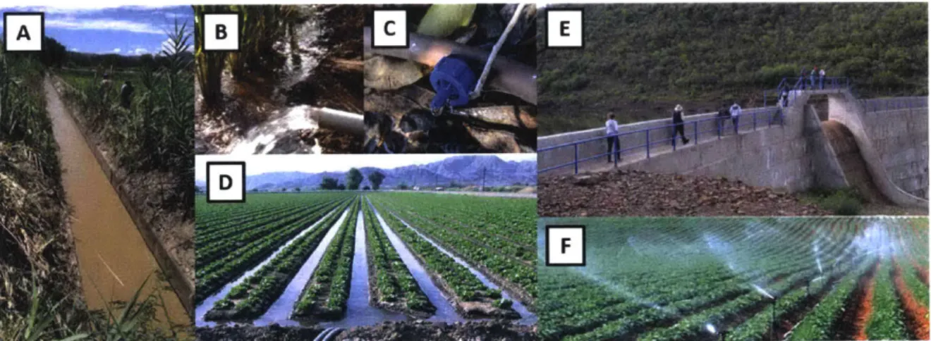
1-1 Examples of various irrigation methods. More traditional methods such as canal (A), flood (B) and furrow (D) irrigation lose water to evaporation and absorption. Methods with a pressurized pipe network include sprinklers (F), which can still lose water to evaporation, and drip (C), which minimizes water loss. Any of these methods can be gravity-fed (E) with an elevated tank or dam. . . . . 24

1-2 An example stakeholder map for the development and distribution of solar powered drip irrigation systems. . . . . 26

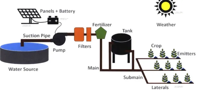
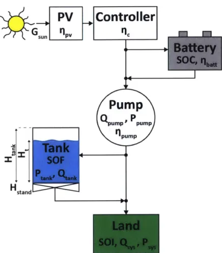
2-1 A diagram of a solar powered drip irrigation system shows the relevant

components and subsystems. . . . . 30

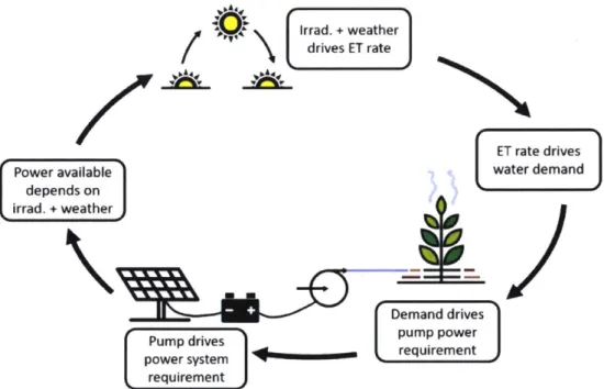
2-2 The cyclic relationship of the four interdependent subsystems. The agronomic requirements of the crop are influenced by local weather patterns, and dictate the hydraulic load on the pump. This in turn dictates the capacity requirements for the power system, which is also dependent on the weather throughout the irrigation season. . . . . 32

(10)

3-1 The system model architecture and its three phases: simulation, design and performance. The modules in the first two phases represent the four subsystems, and the last phases assesses the performance of the proposed system design. A PSO algorithm iteratively proposes designs until the solution converges on the design with the best performance. The performance can either be defined as the life cycle cost, or the profit from crop yield. Note that the crop yield module is only used for the profit-based optimization. . . . . 35

3-2 Field data shows how the daily water demand varies over the season, tracking the available solar irradiance. This illustrates the link between local weather patterns, crop water demand, and the resulting hydraulic load on the system . . . . 37

3-3 An example hydraulic network layout for the 1 ha sample field shows the main pipe (blue), submain pipes (red) and laterals

(black).

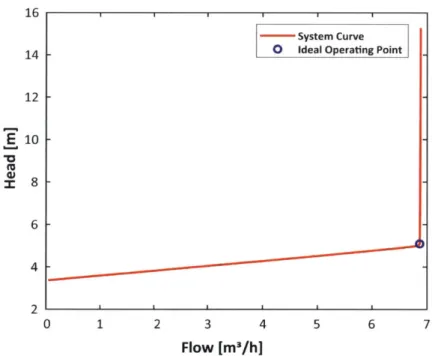
The emitters (not shown) are spaced along the laterals. The pipe diameter decreases for each type of pipe. The network geometry is subjective, but in this study, the laterals are 50 m and the submain lengths are selected to meet the area requirement. . . . . 41

3-4 The hydraulic system curve for the 1 ha sample case shows the pressure compensating behavior introduced by the low pressure PC emitters.

(11)

3-5 A diagram of the design components and their parameters shows how the components relate to one another energetically. The panels are defined by their efficiency, Tpv, the controller is represented by'%, and the battery has a state of charge vector (SOC) and an efficiency, batt. The pump is characterized by its operating point at

Qpump,

Pump, and

its efficiency, 7pump. Water is pumped to the tank at the operating

point

Qtank,

Ptank. The tank has a height, Htank, and its operating pressure depends on the stand height, Htan, the height of the water,

Ht, and its state of fill vector (SOF). The battery and tank are both

optional energy storage options that may be added to the power system design. The drip network operates at Qsz,, Pay,, and there is a state of

irrigation vector (SOI) that describes the volume water delivered to the field at any given time. . . . . 44

3-6 The constant system flow rate, Qy,, is used to select a set of feasible pumps from a database such that the system flow rate is within

65-110% of the pump BEP flow rate. Each pump is assumed to be paired

with a VFD. The system operating point (QSVS, H.y,) is used along with

the centrifugal pump affinity laws to determine the pump operating curve (dotted green line). The operating power, efficiency and NPSHr (red stars) can then be determined. . . . . 47

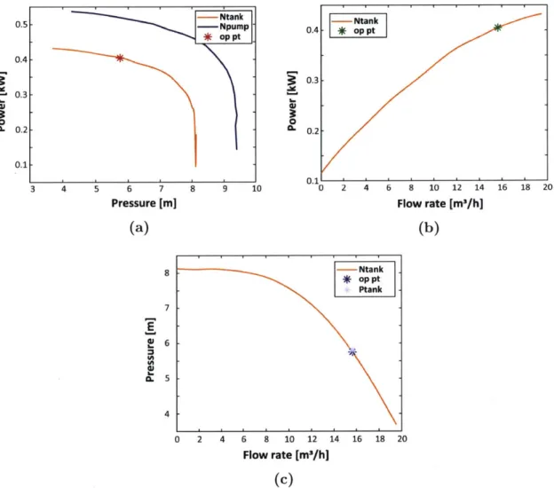
3-7 For designs that include a tank, the pump operation when pumping to the tank must be determined. A constant pumping pressure Piank

is assumed and used with the available power and affinity laws to de-termine the operating speed at each time step (red star). This is used to determine the flow rate to the tank (green star). The calculation can be checked by plotting the corresponding pressure on the pump pressure-flow curve, which should equal Ptank (blue stars). This simu-lation allows the flow rate to vary with available power when pumping to the tank. . . . . 49

(12)

3-8 A snapshot of the simulated pump operation with a tank shows the pump can operate at various flow rates. This enables the system to store energy at times of low irradiance or after the irrigation demand

has been met. The normalized tank SOF fills with Qiank and drains

during irrigation events

(SoI).

. . . . 50 3-9 The single diode model is consistently more accurate in determining

the power output of a PV panel at various irradiance levels (a) and temperatures (b) than the efficiency equation. However, the single diode model is more computationally expensive. Either may be used in the system model to predict the power output of the solar panels. . 52 3-10 The system operation simulation has six possible pathways, with four

that power the system and two that store energy. (1) fills the tank and delivers water to the field. (2) pumps directly to the field and (3) drains the tank to the field. Pathways (1)-(3) also charge the battery when there is enough power. (4) charges the battery and uses it to power pumping directly to the field. (5) charges the battery and fills the tank, and (6) just charges the battery. These pathways are tested in sequence to determine which can be used, and multiple pathways may be used in a given time step. This sequence is fixed and prioritizes irrigating over storing energy. . . . . 53 3-11 An example of how the logic flow determines the system state over

two days. The available solar power (orange) is shown for reference. On March 30th, the system irrigates by first draining the tank, then powering the pump with the battery (3,4). The battery is charged, drained and charged over the course of an irrigation event (6,4,6). The

(13)

3-12 The soil water balance at the crop root zone depends on the evapotran-spiration (ET), irrigation (I), precipitation (P), and root zone depletion

(D,), which is dictated by the readily available water (RAW) and to-tal available water (TAW). Accounting for these parameters on a daily basis allows for a more accurate calculation of the irrigation demand and thus a more finely tuned system design. . . . . 59 3-13 The linear and data fit yield curves for olives show the percent change

in yield as a function of the change in crop evapotranspiration (ET), which is related to crop water demand. The fit curve more accurately characterizes the resistance of olives to water stress for low changes in ET. Below 50% ET it is assumed the yield falls to zero. . . . . 62

4-1 The sensitivity of the optimum life cycle cost (LCC) to field size. The systems are direct drive or have a small energy storage capacity. The bar on the left breaks down the LCC into component costs, showing that the hydraulic network makes up over 50% of the cost in all cases. The bar on the right breaks down the LCC into initial, maintenance, and replacement costs, showing that the initial cost makes up more than 70% of the cost in most cases. The loss of load probability (LLP) hovers between 0.1 and 0.15, reaching a minimum in the 0.75 ha case. 73 4-2 The LCC per ha of the optimal system designs. This shows economies

of scale when expanding up to 1 ha, after which there are diseconomies of scale. For this case study, the 1 ha field has the optimal LCC per ha design . . . . 76 4-3 The sensitivity of the system LCC for the 1 ha sample case to panel

area. Each design is an optimum for a given panel area. For small arrays, batteries and very small tanks are included in the design. The overall minimum cost system is effectively a direct drive system. After this optimum, the LLP drops considerably as more capacity is added to the power system . . . . 78

(14)

4-4 The cost-optimum emitter flow rate for each field area. The 2 Lph emitter is only cost effective for the smallest field because the larger fields would require energy storage to meet the reliability requirement at such a low flow rate. The 8 and 10 Lph emitters are never the opti-mum because the power system capacity required to run at such a high flow rate is expensive. The optimal emitter flow rate of the remain-ing cases oscillates between 4 and 6 Lph, likely because the discrete pump selection becomes the primary cost driver in the optimization. For these field sizes, the mid-range flow rates are optimal. The LCC of each optimum system design is labeled in the plot. . . . . 80

4-5 The LLP limit is varied from 0 to 0.5 for the 0.125, 1 and 2 ha fields to explore the sensitivity of the cost-optimization to the reliability re-quirement. An LLP limit of 0 is the most expensive, but the LCC of the optimal designs drops between 7 and 13% when the LLP limit is increased to 0.1. A small relaxation of the reliability requirement can significantly reduce the optimal system cost. An LLP limit of 0.15 was selected for the cost-optimization based on the olive crop yield curve that shows 100% yield at 85% evapotranspiration, which is a proxy for dem and . . . . 81

4-6 The system designs corresponding to the reliability requirement sweep show that the majority of the systems are direct drive. For an LLP limit of 0, the optimal systems have a panel area of 0.67, 4.3 and 15.3

(15)

4-7 The sensitivity of the optimum profit to field size, where the profit and LCC are normalized to the 1 ha case. The profit-optimization produces direct drive designs with slightly larger panel areas than the cost-optimization. The profit is approximately an order of magnitude larger than the cost, so this optimization scheme is less sensitive to small changes in component capacity. There is no imposed LLP limit; the crop yield model, which links the water delivered directly to rev-enue, acts as the reliability constraint. . . . . 84

4-8 The convergence repeatability of the PSO is tested for the (a) 0.125, (b) 1 and (c) 2 ha field sizes while minimizing LCC. Four combinations of the swarm size, N, and the convergence criterion, e, were each run five times per field. The runs converge on an LCC. Typically, for a larger N and smaller e, it takes longer for the optimization to converge. 87

4-9 The corresponding system designs for the PSO repeat runs minimizing LCC. Aside from a few outliers, the runs converge on approximately the same system design for the (a) 0.125 and (b) 1 ha cases. For the (c) 2 ha case, there seem to be two minimum cost solutions, with the direct drive design having a tighter convergence. A swarm size of N = 50 appears to be too large and worsen the ability of the algorithm to

converge on one solution for a convergence margin of e = 10. N = 20,

e = 10 converged tightly and reliably in a reasonable amount of time, so these parameters were selected for the PSO. . . . . 89

(16)

4-10 The sensitivity of the cost-optimum result to varying weather condi-tions for the 1 ha sample case. The TMY data

(hourly)

produces the most expensive optimum design. The data from two drought years (hourly) produces slightly less expensive designs. The LLP is larger in these years indicating a trade-off between taking advantage of the higher irradiance by reducing panel area and meeting less of the crop water demand. The measured 2018 weather data (five-minute) pro-duces the least expensive design, indicating possible further cost re-duction using higher resolution weather data. The design variation suggests a preliminary "weather robustness factor" of 1.33 for direct drive optimum designs. . . . . 92

5-1 Field trial layout and instrumentation. Data recorded by two pressure sensors (P1, P2) and a flow meter (F) were transmitted every 10 min-utes. A manual pressure gauge (M) was used to verify the last emitter was at activation pressure. The pump operating pressure was set based on the pump house pressure sensor reading when the last emitter was operating at its rated flow. . . . . 95

5-2 The water delivered compared to the simulated demand in Morocco (a) and Jordan (b). The season LLP calculated using the data and simulated demand was zero for both sites because the crops were over-w atered . . . . 96

5-3 The pressure and flow rate measured over the season. The dashed line intersection shows the simulated operating point, and the grey bands show the expected variation range for pressure and flow. The

(17)

5-4 The measured pressure, simulated operating pressure, and expected range. In Saada (a), the pump frequently operates below the simulated value, but within the expected range. In Sharhabeel (b), the pump operates close to or above the upper end of the expected pressure range.

In both cases, the system should have delivered water uniformly. . . . 99

5-5 The pressure drop across the filters and fertigation unit were monitored during the season. The maximum pressure difference is 0.40 bar in Saada (a) and there is a gradual increase in pressure drop from around 0.05 to 0.15 bar, which is likely the sand and disk filter becoming dirty over the season. The maximum pressure difference is 0.25 bar in Sharhabeel (b). Both plots show distinct spikes, which are likely fertigation events. . . . . 99

5-6 The measured flow rate, simulated operating flow rate, and expected range. The points outside of the expected range correspond to lower pressures. Although these pressures are within the expected range, they still could be too low for all the emitters to reach activation. In Sharhabeel (b), the lowest flow rate points correspond to the highest pressure points, indicating some part of the system was partially closed off during testing or start-up. . . . . 100

5-7 The measured electrical power to the pump, simulated operating power, and expected range. For both sites, the measured power is frequently higher than the expected range. There is a higher power requirement than expected because both systems are oversized. The pump is not operating within its POR, and therefore it is operating at a lower effi-ciency than simulated. The average simulated pump effieffi-ciency is 36% for Saada and 40% for Sharhabeel, but the average measured pump efficiency is 27% for both sites . . . . 101

(18)

5-8 Example of a "good" and "bad" solar day. The orange shaded region shows the available power output of the solar panels and the yellow line shows the electrical power consumed by the pump. On a good solar day, the system operation is not limited by the available solar power. On a bad solar day, the system operation is limited. A system may appear to be oversized for the former, but it is sized such that it can reliably operate during the latter. . . . . 102

(19)

List of Tables

4.1 Optimum LCC Design for Various Field Sizes . . . . 75

4.2 Optimum Profit Design for Various Field Sizes . . . . 85

4.3 Weather Data Averages . . . . 90

A.1 Sample Case Definition . . . . 106

(20)

(21)

Chapter 1 Introduction

1.1 Motivation

Globally, an estimated 500 million smallholder farmers work plots of 2 hectares (ha) or less and produce 80% of the food consumed in Asia and Sub-Saharan Africa

[1].

However, only about 10% of global arable land is irrigated

[2].

Irrigation can improve yields and decrease water usage for farmers working small plots of land. Traditional methods of irrigation, such as flood and furrow irrigation, involve pouring large quan-tities of water over the field or into adjacent troughs in the soil. Water can easily evaporate or be absorbed into the soil without reaching the crop roots. If existing agricultural land can be made more productive, the increased output per capita can increase incomes and improve food security.

A drip irrigation system is comprised of a power source connected to a pump that pumps water through a pipe network to the crops. The main pipe connects the pump to the submain pipe, which is connected to lateral pipes that extend along the crop rows. Emitters are attached along the laterals at each crop and release water and nutrients to the root zone of the crop. Pressure compensating (PC) emitters are flow control devices that operate at a relatively constant flow rate above a certain activation pressure. Drip systems with PC emitters can uniformly distribute water to the field, regardless of topology, ensuring that all crops receive the same amount of water. Drip irrigation can reduce water consumption by up to 70% over traditional

(22)

methods, and has been shown to increase crop yields by 20-90%, depending on the type of crop [3, 4, 5, 6, 7]. This is especially important in arid regions that are already experiencing water scarcity.

Despite the benefits of drip irrigation, the high capital cost of the systems makes it difficult for smallholder farmers to adopt the technology [8]. The system cost is sensitive to a complex set of co-dependent factors. Many rural farmers have inter-mittent or no access to grid electricity, which means they would require an off-grid power source, such as solar panels and batteries

[9].

Traditional PC emitters have a minimum activation pressure of 0.5-1 bar to operate at their nominal flow rate, which requires significant pumping power, and therefore more expensive pumps and power systems. This thesis considers a drip system with custom, low-pressure emit-ters that exhibit PC behavior at a minimum pressure of 0.15 bar. This low pressure significantly reduces the pumping power required to operate the drip system

[101.

For a given geographic location and crop type, agronomy parameters and local weather patterns determine the water demand of the plant. This informs the hydraulic system design and pump selection, which in turn dictates the power system requirements. Modeling these components as an integrated system can elucidate trade-offs that cannot be exploited if the components are modeled independent of one another.

This thesis presents the development of a drip irrigation system design tool that produces the optimal low cost system for a given location and crop type. The model simulates the system behavior, selects components and then optimizes for the lowest-cost system design. The extent of the model capabilities is explored through sensitiv-ity analysis. This tool is used to design systems for two field trial locations in Jordan and Morocco, and the data from these trials are used to validate and improve the

(23)

1.2 Drip Irrigation

Traditional irrigation methods include flood, furrow, and canal irrigation. Flood irrigation involves flooding the entire field with water (Figure 1-1B

[11]).

Most of the water is absorbed into the ground away from the crop roots or evaporates, making this an inefficient form of irrigation. In furrow irrigation, channels are cut into the ground alongside the crop rows (Figure 1-1D [12]). These channels are filled with water, and although the absorption is more localized, the water can still be lost to evaporation and absorption where the furrows have not yet reached the crop rows. Canal irrigation improves on this slightly with concrete lined channels that carry the water to unlined channels along the crop rows. This reduces the amount of water lost to absorption, but evaporation is still an issue

(Figure

1-1A). In all three of these methods, the water is exposed to atmospheric pressure, so the distribution of the water to the crops is highly dependent on the field topology, and some sections of the field may routinely receive more water than others.

A sprinkler system is a pressurized method of irrigation that delivers water through a pipe network to sprinklers in the field, which spray water over the crops

(Figure

1-IF

[131).

Due to the pipe network, no water is lost to absorption as it travels to the field, but the water can still evaporate from the sprinklers and wind can blow the water droplets away from the crops. This is a more efficient form of irrigation, but typically more expensive due to the pipe network and sprinklers. In any of these irrigation methods the water may be pumped or gravity-fed. Gravity-fed irrigation involves water stored at a height, which could be in the form of an elevated water tank or an entire dam, depending on the size of the field (Figure 1-1E).

Drip irrigation is similar to sprinklers in that it requires a pipe network, but instead of spraying the water over the crops, drip emitters placed along the pipes at each crop release a controlled volume of water directly to the root zone of the crop (Figure 1-IC). This significantly reduces the amount of water lost to evaporation and absorption away from the crop. Fertilizer is typically introduced into the water source and distributed through the irrigation system in a process called fertigation.

(24)

LU

Figure 1-1: Examples of various irrigation methods. More traditional methods such as canal (A), flood (B) and furrow (D) irrigation lose water to evaporation and absorption. Methods with a pressurized pipe network include sprinklers (F), which can still lose water to evaporation, and drip (C), which minimizes water loss. Any of these methods can be gravity-fed (E) with an elevated tank or dam.

This means drip irrigation systems can deliver an exact amount of nutrients directly to the crops, without runoff or uneven distribution.

Although drip irrigation is a more efficient and controlled irrigation method, it only makes up 6% of the global irrigated area [14]. Drip is not widely adopted among smallholder farmers because of the high initial investment and additional mainte-nance costs [15, 16]. Typically the pressure required for a drip system with existing emitter designs is too high to be gravity-fed. Many smallholder farmers have inter-mittent or no access to electricity, so the power system must be off-grid for reliable irrigation

[9].

Drip systems also require additional maintenance compared to other irrigation methods. Emitters have small internal flow paths, so the water typically needs to be filtered and emitters need to be routinely checked for clogging. All this

(25)

1.3 Stakeholders

The target users of these systems are smallholder farmers who may lack access to the capital and technical knowledge to purchase and maintain drip irrigation systems. Smallholder farmers work less than 2 ha of land, growing crops for either subsistence or profit. In Jordan and Morocco, the two countries considered in this study, there are programs to encourage adoption of more efficient irrigation methods by educating farmers about these technologies and offering subsidies. However, farmers often lack the capital to purchase such systems and have difficulty obtaining loans from banks. Depending on the specifications of the program, this can make it difficult for farmers to take advantage of the subsidies

[15,

16].

The key stakeholders in this process are the company that produces the drip sys-tems, an organizational body that coordinates distribution and subsidies for farmers, and the farmers themselves. The main priorities of each stakeholder have been iden-tified through conversations with two agricultural research organizations: Methods for Irrigation and Agriculture (MIRRA) in Jordan and the International Center for Agricultural Research in the Dry Areas (ICARDA) in Morocco. Jain Irrigation Ltd., the second largest irrigation company in the world, and local smallholder farmers in Jordan and Morocco were also consulted. An example stakeholder map that shows how these groups might interact is given in Figure 1-2.

The priority of the company is to make a profit and continually improve the system design. The priorities of the government agency or NGO are to expand access to more efficient forms of irrigation and conserve water resources. The priority of the users is to increase yield and income, decrease their use of water, fertilizer and other resources, and avoid a high capital investment or added maintenance costs. An irrigation company would design, source, and assemble drip kits for farmers in a specific location. A government agency or NGO would handle distribution of these kits to the farmers and coordinate subsidies for the farmers to encourage adoption. This agency would also collect user feedback and system performance data for the company. A training program must be established to install the systems and provide

(26)

Company

• Manufactures drip kits

• Organizes training program _$$

Training Program Provides training

and maintenance 4- ?

-NGO or Government Agency

• Distributes kits • Provides subsidies FarmersI • Target users $ • Customers _E I -T -- O rip kit nowledge Money ata Maintenance nquiries ransfer ptional transfer

Figure 1-2: An example stakeholder map for the development and distribution of solar powered drip irrigation systems.

farmers with initial training and continued technical support. This program would be organized and funded by the company, potentially with additional funding from the government agency or NGO. This proposed set of stakeholder interactions would ensure that smallholder farmers have access to low-cost drip irrigation technology as well as the knowledge to maintain and profit from it throughout the system lifetime.

1.4 Previous Work

Shamshery (2018) presents a low-pressure, online PC drip emitter design with an activation pressure one seventh that of existing commercial products

[17].

These emitters have been manufactured and tested in the field, as shown in [18], and are used exclusively in the systems-level model presented in this thesis. Their low

(27)

acti-Bakelli (2011), Muhsen (2018), Kelley (2010), Deveci (2015), and L6pez-Luque (2015) all consider the design and optimization of solar powered pumping systems but impose limitations on their models [19, 20, 21, 22, 23]. Bakelli (2011) defines a demand-based reliability constraint and an economics model for calculating the system life cycle cost (LCC), which are useful for framing the optimization problem. The hydraulic behavior of the system is estimated using a polynomial fit to data, rather than fluid mechanics, and the optimization method is a simple minimum point search. This limits the scope of cases the model could design for and the system design space. Muhsen (2017) proposes a multiobjective optimization scheme that minimizes LCC, a reliability metric called the loss of load probability (LLP), and excess water volume. While the optimization algorithm is more advanced, the three minimization criteria are weighted subjectively. The paper also defines the system components a priori, rather than selecting the components within the optimization scheme, and only optimizes for the number of panels and tank capacity. Kelley (2010) assesses the feasibility of solar powered irrigation, assuming a system with a well source, and using average irradiance and maximum crop water requirement for five cases studies. The system designs are not optimized, but local economic data are used to link designs to their locations. This is a concise, first-order assessment that is a useful benchmark for a more detailed sensitivity analysis. Deveci (2015) discusses the design of a low-cost, solar powered drip irrigation system for small farms using a systems-level approach. The study assumes a system that includes batteries and a tank, assumes the irrigation time required and only considers component capital cost. The systems-level approach is useful for framing the problem, but the system description is over-simplified by its assumptions. L6pez-Luque (2015) discusses the optimal design for a solar-powered irrigation system using an olive orchard case study. The paper uses various sub-models to simulate the system while implementing a deficit irrigation scheme and optimizing for profitability. This study shows that with deficit irrigation the cost of the solar-powered pump is able to be reduced, but the model is limited with a very specific system design that does not include energy storage options and only considers non-pressure compensating emitters.

(28)

Other studies focus on specific aspects of this design problem. Almeida (2018) produces a pump selection method for solar powered irrigation systems, with the goal of pumping as much water as possible

[24].

The method suggests pairing a vari-able frequency drive (VFD) with a pump to ensure a wide potential operating range. The method becomes useful in the context of this study when selecting pumps that must pump to the PC drip network as well as to a water storage tank. Villalva (2009) presents a comprehensive and instructional approach to accurately model photovoltaic (PV) array operation under various temperature and irradiance conditions

[25].

Sev-eral studies have explored how to model the life cycle cost of these systems. Lai (2017) and Muhsen (2017) both propose detailed cost models that consider initial investment, maintenance, replacement, interest, and inflation over the lifetime of the system. The cost equations used in this study are based off of these definitions [26, 20].

This study builds upon previous work on solar powered drip irrigation systems by adding resolution and flexibility to the model. Local hourly weather data are used to simulate the PV array behavior and calculate a daily water demand based on crop properties and growth. The behavior of the hydraulic network is simulated using fluid mechanics equations to allow for any pipe network configuration. The custom ultra-low pressure PC emitters used in the model shift the system operating point into a lower pressure regime than a system with conventional PC emitters. The pump selection and power system design are optimized in a particle swarm optimization (PSO). Local economic data are used in a life cycle cost objective function and a limit on the LLP constrains the optimization. By using high resolution datasets and simulating the behavior of the individual system components, this holistic model offers a broader design space to explore and optimizes for a solution that is intrinsically linked to a given location and crop type.

(29)

Chapter 2 System Components

2.1 Drip System Overview

A drip irrigation system consists of a water source, a pump, a power system, a hy-draulic pipe network, filters, a fertigation unit, and emitters (Figure 2-1). The hydraulic components are connected by a network of pipes that have progressively smaller diameters. The main typically has the largest diameter to reduce pressure losses along its length as water flows to the field. A sand and disk filter are typically placed after the pump to reduce emitter clogging. This is followed by a fertigation unit that periodically injects fertlizer into the network. The type, amount and fre-quency of fertilizer depends on the crop. At the field, the submain pipe lies along one dimension of the irrigated plot. The submain can be the same or slightly smaller in diameter than the main. The laterals, which have the smallest diameter, branch off of the submain and run down the rows of crops, with one or more emitters at each crop. The spacing of the lateral rows, the spacing of the emitters along the lateral, and the number of emitters per crop are agronomic parameters that depend on the type of crop and the soil properties. The emitters exhibit PC behavior, which means that above a certain activation pressure, the emitter flow rate is constant. This ef-fectively means the entire drip system will operate at a fixed flow rate. The emitters considered in this work have been designed to operate at 0.15 bar, one-seventh the activation pressure of conventional online PC emitters

[17].

(30)

Panels + Battery0; Fertilizer Weather Tank -Suction Pipe Filters Crop Pump _~Emitters

Water Source Main

Submain

Laterals

Figure 2-1: A diagram of a solar powered drip irrigation system shows the relevant

components and subsystems.

Single-speed AC pumps are ubiquitous and about 62% of the global irrigated area draws from surface water sources [2]. The pressure drop in the hydraulic network will fluctuate over time as the water filters become dirty, the fertigation unit is used and the emitters clog. Therefore, the pump must be paired with a VFD to ensure its operating range can accommodate all the states of the system. The pump also requires a controller that can regulate the pump operation and program the irrigation schedule. The power system consists of a solar panel array and, in some cases, energy storage in the form of a battery, a water tank, or both. It is beneficial to have a Maximum Power Point Tracker (MPPT) attached to the panel array to boost efficiency by ensuring that the panels always output the maximum possible power for the given weather conditions. The selection and capacity of these components is highly dependent on the geographical location and the way the components interact as the system operates, which is discussed in Section 2.2.

(31)

2.2 Subsystems

The irrigation system components can be be grouped into four interdependent sub-systems that interact in a loop: an agronomy subsystem, a hydraulic subsystem, the pump, and the power system. The crop type, growth cycle, and water and nutrient needs, as well as the local weather patterns and soil properties are all agronomic considerations. The local solar irradiance, temperature, wind speed, and humidity will determine the evapotranspiration rate of the crops, and rainfall will offset the amount of water the crop needs from the drip system. The type of crop and soil properties will determine the spacing requirements of the drip network, which will in turn dictate the hydraulic behavior of the system. The crop water demand, emitter properties, and network layout will determine the hydraulic operating point, and the selected pump must be able to operate reliably at this point. The characteristics of this pump will determine the power requirement at different head conditions the pump encounters due to the the filters, fertigation, and emitter clogging. This power requirement will dictate the capacity of the power system components, namely the solar panels, batteries, and tank. Given this is a solar powered system, the irradi-ance and weather patterns will determine the power available to the system, thus completing the subsystem loop (Figure 2-2).

This is a dynamic, interdependent system that makes for an interesting opti-mization problem. The objective is to reduce the total life cycle cost of the system. Although the relationships between the subsystems make modeling more complex, these relationships also introduce design flexibility and expand the solution space. The model can simulate the hydraulic behavior of any hydraulic layout which allows for a variety of crops, hydraulic components, and field shapes and sizes. Calculating the crop water demand using local weather data links the hydraulic load on the sys-tem to the available solar power and ensures the design is customized for a specific location. Battery and tank storage allow for irrigation at times of low irradiance or at night. Due to the PC behavior of the emitters, the flow rate of the drip system is fixed, but the pump could fill a tank quickly at higher flow rates, making use of excess

(32)

rrad. + weather

drives ET rate

ET rate drives

Power available water demand

depends on

irrad. + weather

Demand drives

Pump drives pump power

power system requirement

requirement

Figure 2-2: The cyclic relationship of the four interdependent subsystems. The agronomic requirements of the crop are influenced by local weather patterns, and dictate the hydraulic load on the pump. This in turn dictates the capacity require-ments for the power system, which is also dependent on the weather throughout the irrigation season.

solar irradiance, or slowly at lower flow rates, making use of times of low irradiance when there is not enough power to pump directly to the drip system. The field size, crop water demand, and local weather will together determine the capacities of the power system components. By exploiting the subsystem relationships in simulation, the drip system can be cost-optimized for any given location, crop type, and field layout.

(33)

Chapter 3 Methods

3.1 Model Formulation

The systems-level model optimizes a drip system design for a specific "case," and is divided into modules that represent the subsystems discussed in Section 3. Each mod-ule has a set of inputs, which can include datasets and outputs from other modmod-ules, and a set of outputs which is passed to other modules as inputs or for evaluation. The modules and their inputs and outputs are discussed in detail in the following sections. A case is defined by the location, soil texture characteristics, length and diameter of the main, submains and laterals, crop spacing, emitter properties, the pressure drop across the filters and fertigation unit, and the start date of irrigation.

The architecture of the model can be broadly divided into three phases: sim-ulation, design and performance (Figure 3-1). In simulation, the agronomic and hydraulic behavior of the case is established. Information about the local weather and crop properties, such as growth stages and water requirements, are passed into the agronomy module, which calculates the parameters necessary for the daily crop water demand. In parallel, the dimensions of the hydraulic network and the emitter flow properties are passed into the hydraulic module, which simulates the hydraulic behavior of the network and produces a hydraulic system curve. This module is not limited to PC emitters - it can also simulate non-pressure compensating (NPC) emit-ters, sprinklers, or any other irrigation device that works in a pipe network. Both

(34)

the daily crop water demand and the hydraulic system behavior become inputs for the modules in the design phase. In this phase, a suitable pump is selected based on the pipe network hydraulic requirements. The pump specifications and the local weather data are passed into the power module which sizes a solar panel array, a tank, and a battery. The solar panels are required, but the tank and battery can be omitted to produce a direct drive power system. The power system module also runs a simulation of how this drip system would operate over the course of one growing season. Up to this point, no optimization has occurred. This combination of pump and power system components is just one possible design that must be evaluated in the performance phase. The life cycle cost of the entire drip system and the relia-bility with which it meets the crop water demand are calculated and passed into the crop yield module. This module calculates the yield based on the amount of water delivered to the crops over the simulated season and the predicted revenue over the lifetime of the drip system, assuming that seasonlis representative of how the system will perform every year.

A custom particle swarm optimization (PSO) algorithm is used in MATLAB to generate possible designs and determine the trajectory of the design vector. The details of the optimization are discussed further in Section 3.3. The PSO was mod-ified from an algorithm that was successfully used to cost-optimize solar powered village-scale desalination systems

[27,

28]. The PSO operates between the design and performance phase, iteratively offering designs and evaluating their performance until it converges on a solution (Figure 3-1). The objective of the optimization can either be set to minimize life cycle cost or to maximize the profit over the lifetime of the system. With the former, the crop yield module is not used in the optimization. Crop yield is dependent on many variables, which makes it difficult to model accurately, and data on local crop prices may not always be available. It is useful to estimate the profit a farmer could make with one of these systems, but being able to remove the

(35)

Simulation

Weather Crop properties Agronomy module Water requirement per day Emitter spacing Emitter properties Pipe layout Pipe geometry Hydraulic module System pressure-flow curve

Design

Pump database PV database Pump Irrigationschedule modulee PumpselSolapower

Solar array size Battery capacity Water tank capacity

(

Legend:

User inputs

(Code )

Code Outputs

Capital & lifetime cost

Reliability Crop yield module

Revenue 1W ofit

Performance

Figure 3-1: The system model architecture and its three phases: simulation, design and performance. The modules in the first two phases represent the four subsystems, and the last phases assesses the performance of the proposed system design. A PSO algorithm iteratively proposes designs until the solution converges on the design with the best performance. The performance can either be defined as the life cycle cost, or the profit from crop yield. Note that the crop yield module is only used for the profit-based optimization.

(36)

hydraulic network, once simulated, is considered fixed. The purpose of this is twofold. First, the layout of the hydraulic network is typically left to the discretion of the farmer whose agronomic knowledge and familiarity with the field will inform these decisions. Furthermore, some farmers will already have pipe networks that they use with electric or diesel pumps. Second, the optimum of the hydraulic network is known. For a given field size and crop type, the layout that minimizes pipe materials for the lowest operating pressure will be the most cost effective. In future generations of the model, the hydraulic network can be optimized independent of the rest of the system and the result can still be used as an input to the design phase shown here. Similarly, the simulated operation of the drip system for a season in the power module is predetermined. This means that the operation sequence for powering the pump, filling the tank and charging the battery is fixed. This operation scheme has binary checks based on available solar power and the daily water requirement, but it is not optimized. Eventually the algorithm should be able to make decisions about when and how to operate different components such that the system operation parameters become variables within the optimization.

The first step to using the model is defining a case. For continuity, a sample case has been selected as an example for the remainder of this chapter. The case is a 1 ha field of olive trees in Morocco. The trees have a 5 m by 5 m spacing and there are two low-pressure, PC emitters at each crop. The emitters have a rated flow rate of 8 Lph and an activation pressure of 0.15 bar. The module outputs shown are the results for this case, but would be similar in form for any case.

3.2 Subsystem Modules

(37)

400 1 1 1 5 0 -40 300 -C~ - _{- 30} 200 --020 100

r

> -10 0 0

Figure 3-2: Field data shows how the daily water demand varies over the season, tracking the available solar irradiance. This illustrates the link between local weather patterns, crop water demand, and the resulting hydraulic load on the system.

crop, soil texture, sow date, and irrigation type to be specified. It is important to calculate the water demand on a daily basis, rather than use an average or maximum demand, because it varies with the daily weather parameters such as solar irradiance (Figure 3-2). The water demand calculation does not exactly follow the irradiance, as it is also determined by other weather and crop parameters. The large spikes in the water demand in April and July are due to changes in the water uptake in the root zone of the crop. By using a more detailed calculation, the system design can be more closely tuned to the crop needs. The water demand calculation is discussed further in Section 3.2.6.

In the current model implementation, crop data from

[29]

and typical meteoro-logical year weather files (ASHRAE IWEC2) from

[30]

are used. These weather files give representative hourly average weather values based on weather data collected for that location over at least the past 12 years and up to the past 25 years. The important weather parameters used in this model are air temperature (T), relative humidity (RH), solar radiation (Gsoar), wind speed (u), and precipitation (P). The crop tables, which were created based on similar tables in [29] and [8], include the crop growth stages, root depth, plant height, depletion fraction, and crop coefficients.

(38)

In order to calculate the crop water requirement, it is necessary to compute a water balance on the soil (Section 3.2.6). Part of the water balance is the crop evapotran-spiration

(ET),

which is calculated from the crop coefficient (Kc) and the reference evapotranspiration

(ETo),

shown in Equation 3.1.

ETc = Kc • ETo (3.1)

ETo is the evapotranspiration [mm/day] for a grass reference crop of 0.12 m height.

It is calculated using the meteorological data and the Penman-Monteith equation [29]:

0.4086(Rnet - G) + -yC/(T + 273)u2(es - ea)

6 + y(1 + 0.34u2)

Rnet is the net radiation at the crop surface [MJ/m2_{day], G is the soil heat flux}

density [MJ/m2_{day], T is the daily or hourly average air temperature at 2 m height}

_[

],

u2 is the wind speed at 2 m height

[m/s],

e, is the saturation vapor pressure

[kPa]

at air temperature T, ea is the actual vapor pressure

[kPa],

6 is the slope of vapor

pressure curve [kPa/

]

at air temperature T, y = 0.665 x 10-3 is the psychrometric constant [kPa/

],

and P is the atmospheric pressure [kPaj. Details of the calculations of specific terms in the Penman-Monteith equation can be found in [29], Chapter 3. Meteorological variables are extracted directly from weather data whenever possible. At minimum, temperature, relative humidity, wind speed, and total solar shortwave radiation must be provided in the weather file.

Hourly weather data are adapted to the daily evapotranspiration calculation (Eq. 3.1) as follows. Vapor pressure and the slope of the vapor pressure curve are com-puted using minimum and maximum hourly temperatures and relative humidity levels recorded throughout the day. Net radiation at the crop surface (Rnet) is computed as described in

[29],

with the incoming shortwave radiation taken directly from the

(39)

to each stage (Kc,iniiKc,mid, Kc,end) are pulled from the crop tables. Initial and

mid-season stages have constant coefficients, with a linear change in coefficient during the crop development stage between andKc,midandlateseasonbetween Kc,midand

Kc,end. When climate conditions are different from the climates used for tabulated

Kc values such that RHmin,mean

#

45% or U2,mean

#

2.0m/s, Kc,mid and Kc,end are

adjusted (Eq. 3.3), provided that the tabulated value of Kc,nd(Tab) > 0.45:

Kc,mid/end = Kc,mid/end(Tab)+(0.04(U 2,mean -2) - 0.004(RHmin,mean -45))( )o.3, (3.3)

where Kc,mid/end(Tab) is the tabulated value for Kc,mi or Kc,end, h is the mean plant height during the mid/late-season stage [m] (tabulated), and values of 2,mean

and RHmin,mean are calculated for the corresponding growth stage. Custom crop coefficients and development stage lengths can also be entered directly into the crop tables if more accurate local data is available.

After the daily ETc is calculated for the given crop [mm/day], it is converted to the volume of water that needs to be delivered to the field [m 3_{/day]. Equation}

3.4 describes how to convert irrigation (I) in [mm/day] to a volumetric daily water requirement (Virri).

Virri = fw - Afeid -1/1000, (3.4)

where ft is the soil wetted fraction, which is assumed to be 0.3 for drip irrigation and Afield is the field area that is being irrigated [29]. This calculated daily water de-mand is the key parameter that links the subsequent drip system design to a location and crop type.

3.2.2 Hydraulics

The hydraulics module takes in details about the pipe lengths and inner diameters, as well as the pipe network geometry (Figure 3-1). The pipe layout is set by the

(40)

length of the suction pipe, the length of the main between the pump and the field, and a set of subunits whose area is defined by the length of the submain and the length of the laterals. The spacing of the laterals, the spacing of the emitters along each lateral, and the number of emitters per crop are specified based on agronomic recommendations for the crop. The example case includes two subunits of 0.375 ha and a third of 0.25 ha, with a 5 m by 5 m crop and row spacing and two emitters per olive tree (Figure 3-3). This emitter layout is based on suggestions from local agronomists during the field trials. The pipe lengths and number of subunits are somewhat subjective decisions. In all the simulated cases, the laterals were set to 50 m and the length of the submains were made as long as possible to meet the total area requirement. Increasing the length of the submain will incur less of a pressure loss than increasing the length of the laterals because pressure loss in a pipe scales inversely with the pipe diameter squared, and the laterals have the smallest diameter. Not shown in this schematic are additional hydraulic components that incur pressure losses in the system, namely the disk and sand filters, the fertigation unit, elbows, tees, connectors, and valves. Each hydraulic network will contain different quantities of these additional components, so the total additional pressure losses are estimated as part of the case definition that is passed into the hydraulic module.

The final inputs to the hydraulics module are the emitter properties. PC emitters are flow control devices that operate at a constant flow rate above their activation pressure. A drip network of PC emitters will have a constant flow rate once the emitter at the end of the last lateral, which is the furthest from the pump, has reached this activation pressure. The nominal flow rate, activation pressure, flow coefficient, k, and pressure compensation exponent, x, of the custom low-pressure, PC emitters are inputs to the hydraulic module

[17].

The module simulates the hydraulic behavior

(41)

400- 350-300-

I

250-T200 150- 10050 -01L M________ -250 -200 -150 -100 -50 0 50 100 150 200 250 [im]

Figure 3-3: An example hydraulic network layout for the 1 ha sample field shows the main pipe (blue), submain pipes (red) and laterals

(black).

The emitters (not shown) are spaced along the laterals. The pipe diameter decreases for each type of pipe. The network geometry is subjective, but in this study, the laterals are 50 m and the submain lengths are selected to meet the area requirement.

LrpV2 APmajor = fd D 2 APmajor = K 2 (3.5) (3.6)

The Darcy friction factor,

fd,

for turbulent flow in pipes is calculated using the Swamee-Jain formula (Eq. 3.7), where Re is the Reynolds number, D is the pipe

inner diameter and e is the pipe roughness 132].

164

fd = Re ₂

0.2 x log10 ( (E +

-for Re < 2300 for Re > 2300

The emitter flow behavior is modeled as linear when 0

<

P

<

Pact and as following

the curve

Q

= kP when P > Pact. Here, k is the flow coefficient, x is the pressure

compensation exponent, and Pact is the activation pressure. A constant 0.01 bar is added for the pressure loss due to additional pipe fittings and 0.3 bar is added for the (3.7)

(42)

- System Curve

14 Ideal Operating Point

12 E 8l-o 6 4 2 0 1 2 3 4 5 6 7 Flow [m3 /h]

Figure 3-4: The hydraulic system curve for the 1 ha sample case shows the pressure compensating behavior introduced by the low pressure PC emitters. The flow rate increases with pressure until the last emitter has reached its activation pressure, at which point the flow remains constant. The ideal, minimum power operating point for the system is just after this slope change

(blue

circle).

pressure drop across the filters and fertigation unit. Pressure losses due to flow over the emitters are neglected, and the simulation only models steady state behavior. The hydraulic calculation is run for a range of input pressures until the flow rate solution converges to within 1 L/h of the flow at the entrance of the submain. This iterative flow calculation is discussed in further detail in

[31].

The module outputs the system hydraulic curve, as shown in Figure 3-4. The flow rate is the drip network flow rate and the pressure head is the input pressure to the system from the pump. The flow rate increases gradually until the last emitter, the emitter at the end of the furthest lateral, has reached the activation pressure. As the input pressure increases beyond this point, the flow rate remains constant, which

Development and validation of a systems-level cost optimization tool for solar-powered drip irrigation systems for smallholder farms

Development and Validation of a Systems-Level Cost

Optimization Tool for Solar-Powered Drip Irrigation

Systems for Smallholder Farms

Fiona R. Grant

@

Signature redacted

redacted

...

Signatureredacted

SEP

19

2019

Development and Validation of a Systems-Level Cost

Optimization Tool for Solar-Powered Drip Irrigation Systems

for Smallholder Farms

by

Fiona R. Grant

Abstract

Acknowledgments

Acknowledgment of Joint Work

Contents

List of Figures

(black).

Qpump,

Qtank,

(SoI).

(hourly)

List of Tables

Chapter 1

Introduction

1.1

Motivation

[1].

[2].

[9].

[101.

1.2

Drip Irrigation

[11]).

(Figure

(Figure

[131).

LU

[9].

1.3

Stakeholders

[15,

1.4

Previous Work

[17].

[24].

[25].

Chapter 2

System Components

2.1

Drip System Overview

[17].

2.2

Subsystems

Chapter 3

Methods

3.1

Model Formulation

[27,

Simulation

Design

(

Performance

3.2

Subsystem Modules

r

[29]

[30]

(ET),

(ETo),

[

],

[m/s],

[kPa]

_[