HAL Id: hal-01070827
https://hal.archives-ouvertes.fr/hal-01070827
Submitted on 2 Oct 2014HAL is a multi-disciplinary open access
archive for the deposit and dissemination of sci-entific research documents, whether they are pub-lished or not. The documents may come from teaching and research institutions in France or abroad, or from public or private research centers.
L’archive ouverte pluridisciplinaire HAL, est destinée au dépôt et à la diffusion de documents scientifiques de niveau recherche, publiés ou non, émanant des établissements d’enseignement et de recherche français ou étrangers, des laboratoires publics ou privés.
Density and Distribution Function estimation through
iterates of fractional Bernstein Operators
Claude Manté
To cite this version:
Claude Manté. Density and Distribution Function estimation through iterates of fractional Bernstein Operators. 21st International Conference on Computational Statistics, Aug 2014, Genève, Switzer-land. pp.335-342. �hal-01070827�
estimation through iterates of
fractional Bernstein Operators
Claude Mant´e, Aix-Marseille Universit´e, Universit´e du Sud Toulon-Var, CNRS/INSU, IRD,
MIO, UM 110, Campus de Luminy Marseille, France, [email protected]
Abstract. We describe a method for distribution function and density estimation with Bern-stein polynomials. We take advantage of results about the eigenstructure of the BernBern-stein operator to refine the Sevy’s convergence acceleration method, based on iterates of this opera-tor; the original Sevy’s algorithm is improved by introducing fractional operators. The proposed algorithm has better convergence properties than the classical one; the price to pay is a control-lable loss of the shape-preserving properties of the Bernstein approximation (monotonicity and positivity in the Density Estimation setting). The method is tested on simulated data.
Keywords. Density Estimation, Bernstein operator, root of operators, Bernstein polynomials, Lagrange polynomials
1
Introduction
Bernstein simultaneously introduced in 1912 the polynomials and the operator that bear his name in a famous paper [2]. But, as Farouki [8] noticed, this approximation has been seldom used, due to its slow convergence. For instance, to approach f (t) = t2 on the unit interval with a maximal error of 10−4, we need a polynomial of degree 2500 [8] ! Nevertheless, this
operator (denoted Bn) has attractive shape-preserving properties: if f is positive (or monotone,
or convex), its image Bn[f ] is so (see [5] for further properties). Consequently, the structure of
a distribution function (d.f.) is preserved by Bn; this point strongly motivated the use of the
Bernstein approximation in Density Estimation [19, 1, 3, 12, 13, 14].
Notations
We will work in the Banach space C [0, 1] of continuous functions on [0, 1], equipped with the norm ∥f ∥ := max
2 Density and d.f. estimation through iterated Bernstein Operators
Pnwill be the supplementary of P1in Pn. We will denote F+the closed convex cone of positive
functions of C [0, 1], and F1 the closed convex set of functions of C [0, 1] integrating to 1. Consider an operator U : C [0, 1] → C [0, 1]; for n ≥ 2 (fixed), its restriction to Pn will
be denoted U , and its restriction to P◦ n will be denoted U . For the sake of simplicity, the
restrictions of the identity operator to these subspaces will be denoted 1 instead of 1 or 1;◦ M at (U ; B1, B2) will denote the matrix representation of U with respect to the bases B1 and
B2 of C [0, 1]. We will use the matrix p-norms ∥U ∥p := sup v̸=0
∥U(v)∥p
∥v∥p where ∥v∥p is the usual vector ℓp-norm. Notice that ∥U ∥
1 := max 1≤k≤dim(U)
∑dim(U )
j=1 |Uj,k|, ∥U ∥2 is the spectral norm, and
∥U ∥∞:= max
1≤j≤xdim(U)
∑dim(U )
k=1 |Uj,k| (see [7]).
2
Expression of powers of the Bernstein operator into different
bases
The Bernstein operator Bn: C [0, 1] → C [0, 1] is defined by [4, 15, 18]:
Bn[f ] (x) := n ∑ j=0 wn,j(x)f ( j n) with wn,j(x) := (n j )
xj(1 − x)n−j; its range R (Bn) ⊆ Pn. Cooper and Waldron [4] gave its
spectral decomposition, which can be also written into the form hereunder [16].
Theorem 2.1. The Bernstein operator can be represented in the diagonal form
Bn[f ] = n ∑ j=0 λ[n]j πj[n]⊗ π∗[n]j (Ln[f ]) where f ∈ C [0, 1], λ[n]j = n! (n−j)! nj ∈ ]0, 1] and π [n]
j ∈ Pn are its eigenvalues and eigenvectors,
πj∗[n] is the dual vector of π[n]j , and u ⊗ v∗(w) := u ⟨v∗, w⟩.
We will need the Lagrange interpolation operator (equispaced case) Ln: C [0, 1] → C [0, 1]
defined by: Ln[f ] (x) := n ∑ j=0 ℓn,j(x) f ( j n), with ℓn,j(x) := n ∏ k=0 k̸=j n x − k j − k .
Three bases of Pn will be needed:
1. the Bernstein’s basis Wn:= {wn,j(x) , 0 ≤ j ≤ n}
2. the Lagrange’s basis Ln:= {ℓn,j(x) , 0 ≤ j ≤ n}
3. the eigenvectors of Bn, Π[n]:=
{
πj[n](x) , 0 ≤ j ≤ n}.
Let us denote LW[n]the transformation matrix associated with the bases Lnand Wn, whose
jthcolumn consists in the coordinates of w
n,j in the basis Ln. The following results can be easily
demonstrated [16]: Lemma 2.2. M at ( ◦ Bn; Ln, Wn ) = In and M at ( ◦ Bn; Wn, Wn ) = LW[n].
Thank to this lemma, we obtain for any k ≥ 2 a first matrix representation of Bkn from the diagram:
Bnk: C [0, 1] Ln
−→ (Pn, Ln)−→ (PIn n, Wn) LW[n]k−1
−→ (Pn, Wn) . (1)
Besides, Theorem 2.1 gives an alternative representation of this operator:
Bnk: C [0, 1] Ln −→ (Pn, Ln) LΠ[n] −→ (Pn, Π[n] ) Λk [n] −→(Pn, Π[n] )ΠW[n] −→ (Pn, Wn) (2)
where Λ[n] is the diagonal matrix associated with the vector (
1, 1, 1 − 1/n,(3n − 2)/n2), · · · , n!/nn)
of eigenvalues of Bn, and LΠ[n] and ΠW[n] are transformation matrices associated with the
three bases.
3
Sevy’s sequences for d.f. and density approximation
We saw that in the elementary case f (t) = t2, the speed of convergence of Bn[f ] towards f is
only O[n1][8]; the situation is worse in the special case of d.f.s, since it can be proven [15] that one should rather expect O[√1n
]
. To get a sequence of approximations converging faster than Bn, Sevy [17] proposed to supersede Bn by the iterated operator
IIn:=(1 − (1 − Bn)I
)
(3)
and proved the following result.
Theorem 3.1. ([18], see also [4]) For n ≥ 1 fixed, and any function F defined on [0,1], we have: II n[F ] − Ln[F ] −→ 0 I→∞ .
Such a sequence build a bridge between I1n[F ] = Bn[F ] and Ln[F ]. It is worth noting
that Ln[F ] interpolates the data but can be very bumpy and that in the equispaced case, the
interpolation errors are maximal ([6, Ch. 2]; [11, Ch. 5]). Suppose now F is a d.f.; Bn[F ] is also
a d.f., but in general Ln[F ] will not share the same characteristics. Thus, it is natural to try to
determine some optimal number of iterations I∗≥ 1 in order that IIn∗[F ] has the structure of a d.f., while II∗+1
n [F ] has not. In other words, the density approximation cfn (I∗)
(x) := dxdIIn∗[F ] (x) should be bona fide, i.e. should belong to F+∩ F1, while cf
n (I∗+1)
/
4 Density and d.f. estimation through iterated Bernstein Operators
4
Interpolating Sevy’s sequences (see [16])
To refine Sevy’s sequences, we build for K ≥ 2 the Kth “root” of the operator G
n:= (1 − Bn)
involved in Formula 3. Because Bn only preserves P1, the eigenvalues of Gn belong to ]0, 1[.
Thus, thanks to classical results about convergent series of operators (see [10] for instance), one may consistently define the fractional operator
Gn(1/K):= exp ( 1 Klog ( Gn) ) . (4)
One can easily verify the following lemma.
Lemma 4.1. ∀ I ≥ 1, IIn=(1 − (1 − Bn)I ) = ( 1 − ( 1 −B◦n )I) ◦ Ln.
Consequently, we can proceed as if f ∈ R (Ln) and don’t have to worry about the “Lagrange
residual” f − Ln[f ]. Since P1 is preserved by Bn and because of Lemma 4.1, Ikn(f ) = L1[f ] +
Ikn(Ln[f ] − L1[f ]), and we can set the definition of K-fractional Sevy’s sequences.
Definition 4.2. Let K ≥ 2, and f ∈ C [0, 1]. The K-fractional Sevy’s sequence of approxima-tions of f is: Ijn;K[f ] := L1[f ] + ( 1 − Gn(j/K) ) (Ln[f ] − L1[f ]) , j ≥ 1.
Such a sequence interpolates the original one, since Ij Kn;K[f ] = Ijn(f ). Its matrix
representa-tion stems from diagram 2.
Lemma 4.3. M at (◦ I j n;K; Ln, Wn )
= ΠW[n]◦Λ(j/K)[n] ◦LΠ[n], where Λ(j/K)[n] is the diagonal matrix
associated with the vector
( 1, 1, 1 − ( 1 n )(j/K) , 1 − ( 3n − 2 n2 )(j/K) , · · · , 1 − ( 1 − n! nn )(j/K)) .
5
Numerical issues
Because of Lemmas 2.2 and 4.1, building a classical Sevy’s sequence amounts to compute powers of the transformation matrix LW[n] (see diagram 1). The condition number of this matrix in the ℓ2-norm is [7]: ∥LW[n]∥2 LW −1 [n] 2 =λ[n]0 λ[n]n = nn!n ≈ √en
2πn (asymptotically - see [9]). Thus, LW[n] is
ill-conditioned, and one must expect to meet numerical problems when n is big. The situation is potentially worse for fractional sequences, since Lemma 4.3 shows that the matrix of the restricted operator depends on both the ill-conditioned transformation matrices LΠ[n]and ΠW[n]
(see Figure 1).
Figure 1. Logarithm of the condition numbers of the transformation matrices P L[n], P Π[n] and LW[n] ; the continuous line corresponds to the asymptotic value n −12Log (2πn).
òò òò òò òò ò òò òò òò òò òò ò òò òò òò ò òò ò òò òò ò ôô ôô ôô ôô ôô ôô ôô ôô ôô ôôô ôôô ôôô ôôô ôô ôô ô æ ææ æ æ ææ æ æ ææ æ æ ææ æ ææ æææ æææ æææ æææ æææ ææ 0 5 10 15 20 25 30 35 0 10 20 30 40 50 60 70
{2-norms of the transformation matrices
ò PL
ô PP
æ LW
But the point for us is merely to control numerical errors in computing Ijn;K[f ]! No-tice that on the one hand M at
(
◦
Bn; Ln, Wn
)
= In (Lemma 2.2), while on the other hand
M at ( ◦
Bn; Ln, Wn
)
= ΠW[n]◦ Λ[n]◦ LΠ[n] (diagram 2). Consequently, the matrix norms ΠW[n]◦ Λ[n]◦ LΠ[n]− In 1 ΠW[n]◦ Λ[n]◦ LΠ[n]− In ∞ (5)
are convenient indicators of loss of numerical accuracy imputable to the ill-conditioning of the transformation matrices. Since the only easy-to-handle basis is the power basis, the transforma-tion matrices P L[n], P Π[n] and P W[n] are straightforwardly computed, and we can write:
ΠW[n]= P Π−1[n] ◦ P W[n]
LΠ[n]= P L−1[n] ◦ P Π[n] (6)
(formally). But we can derive from Figure 1 that these inverse matrices cannot be computed with sufficient accuracy in general. Thus, it’s necessary to supersede in (6) the inverse matrices by the Moore-Penrose generalized inverses P Π+[n] and P L+[n]. This gives rise to the regularized operators:
g
ΠW[n]:= P Π+[n]◦ P W[n] f
LΠ[n]:= P L+[n]◦ P Π[n]. (7)
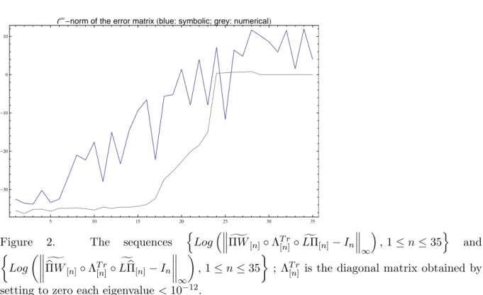
On Figure 2, we plotted the logarithm of the second indicator of Formula (5), for n ranging from 1 to 35 (a similar graph can be obtained for the first indicator). Two cases must be distinguished on this plot: the “symbolic” one, where polynomial eigenfunctions were computed from the recurrence formula given by [4], and the “numerical” one, where they were computed by polynomial interpolation of the eigenvectors of LW[n], giving rise to the alternative basis
b Π[n] :=
{ ˆ
6 Density and d.f. estimation through iterated Bernstein Operators 5 10 15 20 25 30 35 -30 -20 -10 0 10 {¥
-norm of the error matrixHblue: symbolic; grey: numericalL
Figure 2. The sequences {Log( gΠW[n]◦ ΛT r[n]◦ fLΠ[n]− In
∞ ) , 1 ≤ n ≤ 35} and { Log( ΠWbg[n]◦ ΛT r [n]◦ fLbΠ[n]− In ∞ ) , 1 ≤ n ≤ 35 } ; ΛT r
[n] is the diagonal matrix obtained by
setting to zero each eigenvalue < 10−12.
not different roundoff errors on both sides, imputable to different algorithms! That is why we took into account the numerical rank of B◦n, discarding from the computation of Formula (5)
eigenvectors associated with eigenvalues smaller than 10−12 (see Figure 2 and its legend).
It is worth noting that the computational cost in the symbolic case is considerable: it took about 6600 seconds to produce the symbolic part of Figure 2, while the numeric part was obtained in 80 seconds.
6
Application to density an d.f. estimation
Suppose F is some differentiable d.f. associated with a random variable X defined on [0, 1], and that SN := {X1, · · · XN} is a N -sample of X, giving rise to the empirical d.f. FN(x). Babu et
al. [1] proposed to estimate F by a Bernstein polynomial eFN,m of degree m:
e FN,m(x) := m ∑ k=0 FN( k m) wm,k(x) = Bm[FN] (8)
with m ≤ m0 := ⌈N/Log (N )⌉. The proposed method consists in superseding Bm0[FN] by some IIm∗∗;K[FN], where m∗ ≤ m0 and I∗≥ K (fixed) are convenient values of the degree of the estimator and of the number of iterations in Definition 4.2.
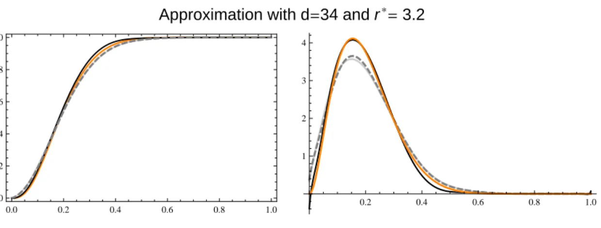
As an illustration, we displayed first on Figure 3 the results obtained with a sample of size 200 of β (3, 12), with K = 10. We found that I∗ = 32 iterations of the fractional operator (4)
simultaneously corresponded to a satisfactory fit of the e.d.f. and an approximately bona fide density estimation. Thus, in this case, the fractional number of iterations was r∗ = 1 + 2210. On this plot, we superimposed to the true d.f. three estimators: the Babu’s one, of degree m0 = 38,
Figure 3. Estimation of the β (3, 12) d.f. and density from a sample. Left panel: the true d.f. (orange), the Babu’s one (gray and dashed, of degree m0 = ⌈200/Log (200)⌉ = 38), the classical
Bernstein estimator of degree m = 34 (gray), and the proposed one (black), of degree 34 too. Right panel: density estimators obtained by deriving the d.f.s estimated.
0.0 0.2 0.4 0.6 0.8 1.0 0.0 0.2 0.4 0.6 0.8 1.0 0.2 0.4 0.6 0.8 1.0 1 2 3 4
Approximation with d=34 and r*=3.2
the Bernstein estimator of degree m = 34, and the iterated estimator (black), of degree 34 too. The density estimators are derivatives of these d.f.s
In addition, we collected in Table 1 results from simulations carried on with 30 samples of size N = 150 (⇒ m0 = 30) of four Beta distributions. For sake of simplicity, we fixed I∗ = 20
(see [16] for a theoretical justification). For each one of these samples and for each estimator (4 estimators of the d.f. and 3 estimators of the density, since the e.d.f. is not differentiable), the Integrated Squared Error (ISE)∫ ( ˆF (x) − F (x))2dx and the L1 error norm∫ ˆf (x) − f (x) dx were computed. Clearly, even in this suboptimal situation (I∗ = 20 ), the proposed estimators
outperformed classical ones, excepted in the very simple case β (1, 2) (uniform distribution). Notice the honorable performances of the good old e.d.f.! 1
Table 1. Simulations results. First group of colums: the distribution simulated, and optimal value of m (for further details, see [16]); second group: median of 103.ISE of estimated distri-bution functions; third group: median of the L1 error norms for estimated densities. Best result
are in bold characters.
Probability m∗ e.d.f. B30 Bm∗ I20m∗ B′30 Bm′ ∗ I′20m∗ β (1, 2) 16 0.497 0.415 0.38 0.569 0.1 0.09 0.108 β (2, 4) 18 0.6 0.51 0.56 0.368 0.108 0.12 0.099 β (3, 12) 25 0.32 0.783 0.908 0.258 0.197 0.207 0.118 β (10, 10) 25 0.318 1.16 1.37 0.289 0.248 0.263 0.153
Bibliography
[1] Babu, G. J., Canty, A. J. and Chaubey, Y. P. (2002) Application of Bernstein polynomials
for smooth estimation of a distribution and density function. Journal of Statistical Planning
8 Density and d.f. estimation through iterated Bernstein Operators
and Inference, 105, 377-392.
[2] Bernstein, S. N. (1912) D´emonstration du th´eoreme de Weierstrass fond´ee sur le calcul des
probabilit´es. Commun. Soc. Math. Kharkov, 13, 1-2.
[3] Bouezmarni, T. and Rolin, J.M. (2007) Bernstein estimator for unbounded density function. Journal of Nonparametric Statistics, 19, 3, 145-161.
[4] Cooper, S. and Waldron, S. (2000) The eigenstructure of the Bernstein operator. Journal of Approximation Theory, 105, 133-165.
[5] Davis, P. J. (1963) Interpolation and approximation. Blaisdell, New York
[6] de Boor, C. (1978) A practical guide to splines. Applied Mathematical Sciences, 27, Springer-Verlag, New York.
[7] Farouki, R. T. (1991) On the stability of transformations between power and Bernstein
polynomials forms. Computer Aided Geometric Design, 8, 29-36.
[8] Farouki, R.T. (2012) The Bernstein polynomial basis: a centennial retrospective. Computer Aided Geometric Design, 29, 379-419.
[9] Impens, C. (2003) Stirling’s series made easy. Amer. Math’l Monthly, 110, 730-735. [10] Kato, T. (1995) Perturbation theory for linear operators. Springer-Verlag, Berlin,
Heidel-berg.
[11] Laurent, P.-J. (1972) Approximation et optimisation. Enseignement des sciences, 13, Her-mann, Paris.
[12] Leblanc, A. (2010) A Bias-reduced approach to density estimation using Bernstein
polyno-mials. Journal of Nonparametric Statistics, 22, 4, 459–475.
[13] Leblanc, A. (2012) On estimating distribution functions using Bernstein polynomials. Ann. Inst. Stat. Math., 64, 919-943.
[14] Leblanc, A. (2012) On the boundary properties of Bernstein polynomial estimators of density
and distribution functions. Journal of Statistical Planning and Inference, 142, 2762-2778.
[15] Mant´e, C. (2012) Application of iterated Bernstein operators to distribution function and
density approximation. Applied Mathematics and Computation, 218, 9156-9168.
[16] Mant´e, C. (in revision) Iterated Bernstein operators for bona fide distribution function and
density estimation. Balancing between the iterations number and the polynomial degree.
[17] Sevy, J. C. (1993) Convergence of iterated boolean sums of simultaneous approximants. Calcolo, 30, 41-68.
[18] Sevy, J. C. (1995) Lagrange and least-squares polynomials as limits of linear combinations
of iterates of Bernstein and Durrmeyer polynomials. Journal of Approximation Theory, 80,
267-271.
[19] Vitale, R.A. (1975) A Bernstein polynomial approach to density function estimation. Sta-tistical Inference and Related Topics, 2, 87-99.
![Figure 1. Logarithm of the condition numbers of the transformation matrices P L [n] , P Π [n] and LW [n] ; the continuous line corresponds to the asymptotic value n − 1 2 Log (2πn).](https://thumb-eu.123doks.com/thumbv2/123doknet/14743446.577273/6.892.106.567.215.494/figure-logarithm-condition-transformation-matrices-continuous-corresponds-asymptotic.webp)