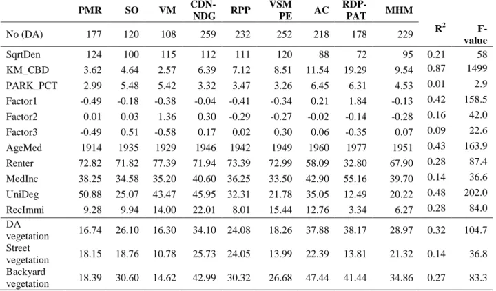
Table 1. Mean values and ANOVA coefficients of the independent variables and three dependent variables by borough (see variable labels, borough names and units in Table 4)
6
0
0
Texte intégral
Figure
+3
Documents relatifs
