HAL Id: hal-00473119
https://hal.archives-ouvertes.fr/hal-00473119
Submitted on 14 Apr 2010
HAL is a multi-disciplinary open access
archive for the deposit and dissemination of
sci-entific research documents, whether they are
pub-lished or not. The documents may come from
teaching and research institutions in France or
abroad, or from public or private research centers.
L’archive ouverte pluridisciplinaire HAL, est
destinée au dépôt et à la diffusion de documents
scientifiques de niveau recherche, publiés ou non,
émanant des établissements d’enseignement et de
recherche français ou étrangers, des laboratoires
publics ou privés.
Networks
Tahiry Razafindralambo, Isabelle Guérin-Lassous
To cite this version:
Tahiry Razafindralambo, Isabelle Guérin-Lassous. SBA: A Simple Backoff Algorithm for Wireless
Ad Hoc Networks. NETWORKING, May 2009, Aachen, Germany. pp.416-428,
�10.1007/978-3-642-01399-7_33�. �hal-00473119�
Ad Hoc Networks
Tahiry RAZAFINDRALAMBO1 and Isabelle GU´ERIN LASSOUS2
1
INRIA Lille - Nord Europe / CNRS / Universit´e Lille 1 tahiry.razafindralambo@inria.fr
2
Universit´e de Lyon / LIP / INRIA isabelle.guerin-lassous@ens-lyon.fr
Abstract. The performance of ad hoc networks based on IEEE 802.11 DCF degrade when congestion increases. The issues concern efficiency and fairness. Many solutions can be found at the MAC layer in the literature, but very few solutions improve fairness and efficiency at the same time. In this paper, we design a new backoff solution, called SBA. SBA uses only local information and two contention window sizes. By simulations, we compare SBA with IEEE 802.11 and several alternatives to 802.11 in ad hoc networks. We show that SBA achieves a good trade-off between fairness, simplicity and efficiency.
Key words: Ad hoc Networks, MAC protocol, Backoff Algorithm
1
Introduction
An ad hoc network is a collection of nodes that communicate via wireless links in a multihop fashion without any fixed infrastructure or centralized servers. An ad hoc network has many practical applications including emergency/rescue operations, military operations and personal area networking.
One challenge in designing protocols for such a network is Medium Access Control. The IEEE 802.11 standard provides a communication mode called DCF (Distributed Coordination Function) that is fully distributed and usable in ad hoc networks [1]. However, the MAC protocol described in DCF exhibits some performance issues in terms of efficiency (often given as the overall throughput in the network) and fairness [2]. If some stations cannot access to the medium or cannot send its packets successfully, these nodes can disconnect the network. Such a disconnection may affect the behaviour of the whole network or prevent some nodes from providing a given service. On the other hand, if fairness and efficiency are achieved, QoS guarantees may be expected and/or provided by/for upper layer and thus for the user application.
Many works have tackled the problem of fairness and efficiency in ad hoc networks. Some approaches modify the BEB (Binary Exponential Backoff) al-gorithm of IEEE 802.11 to provide better performance, whereas ohers introduce new mechanisms. Most ot the existing solutions provide either efficiency or fairness, but very few solutions consider both of them.
In this article, we propose a new approach for a backoff-based algorithm for ad hoc networks, called hereafter SBA for Simple Backoff Algorithm. Our solution relies only on local information, as successful transmissions and collisions under-gone by each station without taking advantage of the carrier sensing mechanism nor the packets that can be decoded. Contrary to the BEB algorithm, SBA has only two distinct contention window sizes. SBA also uses the same contention window for all the packets it has to send in a given time interval. At the end of this interval, some computations are done to choose the contention window for the next interval. The first results show that SBA is a good candidate in terms of trade-off between fairness, simplicity and efficiency.
After a state-of-the-art given in Section 2, SBA is described in Section 3 . Then, the protocol is evaluated by simulation. The results are given in Section 4. We compare SBA with 802.11 and some other fair MAC protocols. Finally, we give a preliminary study on the complexity of these protocols in Section 5.
2
Related work
Due to space limitation, we only cite works that focus on the fairness issue in ad hoc networks and that design single channel and single interface MAC protocols. There are mainly two categories of MAC protocols in the literature. The first one is based on the backoff mechanism: the protocol uses the contention window to modify the behaviour of the protocol. The use of the contention window can be a modification of the window size or of the way of increasing/decreasing it. The protocols that belong to this category are mainly based on the DCF of IEEE 802.11 for the medium access method. The second category consists of protocols that do not use the backoff algorithm to modify their behaviour. This does not mean that there is no backoff algorithm but the main changes and evolutions inside the protocol are not made via the backoff.
Backoff-based approach: The protocols in this category can be also di-vided into two classes. The first class, called BEB-like algorithms, contains the backoff algorithms that behave like the BEB algorithm: this means that, di-rectly after a successful transmission, the contention window is decreased, and after a collision, the contention window is increased. The MILD (Multiplicative Increase Linear Decrease) algorithm [3] and the DIDD (Double Increase Double Decrease) algorithm [4] belong to this category. Surprisingly, in the literature, most of these algorithms are mainly designed for single-hop networks, and very few of them are tested in ad hoc networks conditions.
The protocols of the second class modify the contention window based on some computations made by the station. These computations use some infor-mation gathered by each station from its neighbourhood. For example, in MB-FAIR [5], the algorithm computes what the authors call a fair share and mod-ifies the contention window size accordingly. The fair share is computed based on some information received from the two-hop neighborhood. The protocols described in [6, 7] also belong to this category.
Other approach or non backoff-based approach: In this category, there are also two main classes of protocols. The first class uses some information other than the one initially provided by 802.11. In the protocol EHATDMA [8], a handshake in EHATDMA can be initiated by the sender or the receiver. The protocols of this category use broad information to provide fairness for all sta-tions.
The protocols of the second class do not use any extra information except the information gathered from the active carrier sensing mechanism. For instance, the protocols PNAV [9] and MadMac [10] belong to this category. MadMac and PNAV insert a waiting time before sending a packet with 802.11. The waiting time is inserted depending on the activity perceived on the medium.
3
SBA: a Simple Backoff Algorithm
3.1 Basic issues with 802.11
(a) The hid-den terminals.
(b) The asymmet-ric hidden termi-nals.
Paire 0 Paire 1 Paire 2
(c) The three pairs.
Fig. 1.Basic configuration issues with IEEE 802.11 DCF
We describe here some basic ad hoc configurations that present performance issues when 802.11 is used. These configurations are often sub-configurations of larger ad hoc topologies. We think that a good understanding of these basic scenarios is important because the rules of our algorithm SBA are based on these issues. We describe three configurations: hidden terminals, asymmetric hidden terminals and the three pairs.
a) The hidden terminals configuration is given on Figure 1(a): the two trans-mitters are independent and try to send packets to the same receiver. The col-lisions due to concurrent transmissions lead to a throughput degradation and a short term unfairness as described in [11]. The collisions may be reduced with the RTS/CTS mechanism of 802.11. b) The asymmetric hidden terminals con-figuration is given on Figure 1(b): the transmission of the upper emitter always collides and the transmission of the lower emitter always succeeds. This asym-metry leads to a long term unfairness between the two transmitters when 802.11 is used and the RTS/CTS mechanism does not solve the problem [3]. c) The three pairs scenario is presented on Figure 1(c): there is no collision issue, but unfairness arises with 802.11 because the central pair cannot access the medium due to asymmetric contention [12].
3.2 Principles
In SBA, we keep the main principles of the MAC protocol of IEEE 802.11 DCF: a packet is emitted on the radio medium after a DIFS and a backoff time (dur-ing which the medium must be free) and in unicast mode, the data packet is acknowledged after a SIFS. The main differences between SBA and 802.11 are the number of backoff stages and the conditions that determine the contention window size to use. Due to space limitations, we do not describe IEEE 802.11 DCF (see [1] for more details).
Only two states. Compared to 802.11, SBA has only two different contention
window sizes, one large called hereafter CWmaxand one small called CWmin.
Local information. Our protocol relies only on local information. What we mean by local information is information that a station can derive from its
own experience without using any measure from the carrier sensing mechanism3
and without exploiting the content of the packets it receives nor the packets it can listen on the radio medium. Therefore the used information is collisions and successful transmissions undergone by the station, as done in the DCF mode. There are many advantages in using such local information. For example, such information is always available and reliable and if no message is exchanged the protocol overhead is reduced. Not using the carrier sensing mechanism, for computing the medium occupancy ratio for instance, can be also of some interest concerning the energy consumption. But using only local information has also some drawbacks. For example, when the number of stations is not known, it is difficult for the protocol to have an optimal behaviour. However locality is an important property for ad hoc networks protocols, especially for MAC protocols. How to use local information? The BEB algorithm of IEEE 802.11 is said to be aggressive due to the adaption of the contention window size after a suc-cessful transmission. Many BEB-like algorithms try to cope with this aggressive behaviour by a slow reduction of the contention window size. As SBA has only two distinct contention window sizes, we do not adapt the contention window size after each transmission, in order to reduce the oscillations between these two states. SBA uses the local information gathered during a given time interval to adapt the contention window for the next time interval. The length of this interval must not be too short to avoid possible oscillation and not be too long to increase the reactivity of the algorithm. The time interval used in SBA is fixed and the same for all stations. This interval is called ∆ hereafter.
Computing medium state probabilities. The medium can have different states. From the station point of view, the medium can be occupied by other stations, or occupied by its transmission resulting in a successful transmission or in a collision, or the medium can be idle. We denote the probability for the medium to be in each state by P [occ], P [suc], P [col] and P [f ree] respectively. These four probabilities cannot be accurately computed by using only local in-formation as defined previously. However they can be approximated with this
3
Note that SBA uses the carrier sensing mechanism for accessing the medium to check whether the medium is free or not, but does not make any measure, as the medium occupancy ratio for instance, with this mechanism.
local information. The local information, known and used by a station, is the length and the time needed to transmit each packet. The value of P [suc] for a given interval is thus given by:
P[suc] = Tsuc
∆ (1)
where Tsuc is the time spent by a station in successful transmissions. In the
same way, we can compute P [col] based on Tcol, where Tcolis the time spent by a
station in collisions. Another local information used by a station is the number of successful transmissions and the number of collisions it undergoes during ∆,
and denoted by Nsucand Ncol(resp.). As SBA uses only one contention window
size during a given time interval, it is possible to approximate, during a given ∆ and without sensing the medium, the period during which the medium is idle, denoted by P [f ree], by:
P[f ree] =(Ncol+ Nsuc) × (cw + DIF S)
∆ (2)
where cw is the mean backoff time. This value is an approximation, because, we use the mean backoff time and because it only takes into account the free periods just before the transmissions. Based on previous equations, we can compute P [occ] by using the following relation:
P[occ] = 1 − (P [suc] + P [f ree] + P [col]) (3)
Note also that when the network is unsaturated, the value of P [occ] (P [f ree] resp.) is not the real occupation (idle period resp.) of the medium. This be-haviour is due to the fact that the station does not use the carrier sensing mechanism to define free periods and thus occupation periods, but only local information. However, we will see that this approximation ensures good perfor-mances to SBA in unloaded networks.
3.3 SBA: the protocol
The code of SBA is presented in Algorithm 1. As we have only two states, the algorithm can be seen as the transition between these two states. Algorithm 1 shows how the statistics gathered during the ∆ period are used to switch from one state to another.
Algorithm 1 consists of two main cases given in Line 1 and Line 9. If the condition of Line 1 is true, it means that the station’s occupancy with successful transmissions is lower than the other stations’ occupancy and then its contention
window is set to CWmin (Line 2), otherwise it is set to CWmax (Line 10).
This condition ensures that a node does not monopolize the medium as in, for instance, the three pairs or asymmetric hidden nodes scenarios. If a node thinks that it uses too much the radio medium, then it slows down its emissions by using CWmax.
The condition of Line 1 does not take into account the medium load. The medium load is considered in the condition of Line 6 with two cases. If the
Algorithm 1 SBA
1:if (P [suc] ≤ P [occ] + P [f ree]) then
2: CW← CWmin
3: if (P [col] > r && rand{0,1}=1) then
4: CW← CWmax
5: end if
6: if ((P [f ree] ≤ s && P [col] > 0) || (Nsuc+ Ncol= 0)) then
7: CW← CWmax
8: end if
9:else
10: CW← CWmax
11: end if
medium is heavily loaded, then free periods are reduced and the collision prob-ability is greater than 0 and/or the station can not access to the medium. When these two conditions are satisfied, the station uses CWmax.
The condition of Line 3 uses a random variable to create asymmetry when the probability of collisions is greater than r. In this case, a random variable is
drawn, and depending on its value, the contention window is set to CWmax or
left to CWmin. When the collision probability is very high, it means that there is problem of symmetry in the network. This symmetry appears when the stations use the same contention window size, especially CWmin. If these configurations lead to a high collision probability, this is probably due to the value of CWmin which cannot solve the collisions. In this case, this random drawing tries to break the symmetry and divides by two the number of stations that can potentially use CWmin, which may reduce the number of collisions in the next period. This condition should solve hidden nodes configurations.
4
Simulation results
In this section we present the simulation results of SBA. The simulations are realized on different ad hoc scenarios. We selected scenarios presented in the literature, most of them can be found in [2].
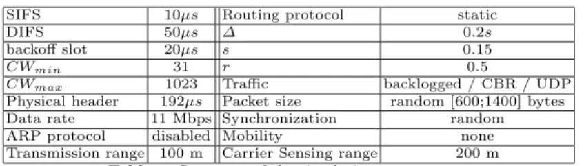
4.1 Simulation parameters
The simulations presented in this section were run with NS-2 [13]. We modified the simulator to reflect the DSSS modulation described in 802.11b. We also removed the overhead due to the routing protocol and the ARP protocol in order to better understand the behavior of SBA. Table 1 gives the summary of
the simulation parameters we use by defaults4. These parameters are used in all
simulations if changes are not specified.
We compare SBA to other MAC layer solutions, including the IEEE 802.11 DCF, MBFAIR [5], PNAV [9], MadMac [10] and DIDD [4]. These protocols belong to different categories of MAC protocols presented in Section 2. We also
4
Due to space limitation, we do not discuss the possible values for the SBA parame-ters. The results are given with a single set of values.
SIFS 10µs Routing protocol static
DIFS 50µs ∆ 0.2s
backoff slot 20µs s 0.15
CWmin 31 r 0.5
CWmax 1023 Traffic backlogged / CBR / UDP
Physical header 192µs Packet size random [600;1400] bytes
Data rate 11 Mbps Synchronization random
ARP protocol disabled Mobility none
Transmission range 100 m Carrier Sensing range 200 m
Table 1.Summary of the simulation parameters.
evaluate SBA when the ∆ periods of all the nodes are synchronized, called SBA sync hereafter. Of course, it is difficult to achieve such a synchronization in ad hoc networks, but this evaluation shows the upper bound on SBA performance. The studied results are the global throughput and the fairness of these protocols. The global throughput, i.e. the sum of the throughputs of all the stations, corresponds to the efficiency of the protocol. We measure fairness, according to the Jain fairness index defined in [14]. When this index is close to 1, it means that the protocol is fair according to a fairness scheme. We use the Max-Min fairness scheme as a baseline comparison, as many studies on fairness in ad hoc networks
do5.
4.2 Performance results
Specific ad hoc scenarios
The 3 pairs The results of efficiency and fairness for the three pairs scenario, depicted in Figure 1(c), are given in Figure 2. In this scenario, the protocol is fair (under a Max-Min fairness scheme) when the throughputs obtained by the three pairs are roughly the same.
0 0.2 0.4 0.6 0.8 1 1.2
MBFAIRMadMacPNAV SBA syncSBA802.11 DIDD MBFAIRMadMacPNAV SBA syncSBA 802.11 DIDD 0 2000 4000 6000 8000 10000 12000 Fairness Index Aggregate throughput (kbps) Efficiency Fairness
Fig. 2.Simulation results for the three pair scenario.
This figure shows that the fairness index of SBA is close to 1, therefore SBA is fair, like MBFAIR, MadMac and PNAV. In this scenario, the three pairs alternate
the use of CWminand CWmax. This alternation allows the central pair to access
the medium more often than with 802.11, which increases the throughput of the central pair and decreases the throughputs of the two external pairs. The
5
flows throughput are roughly equal, which is not the case for 802.11 (or DIDD). On the other hand, the throughput reduction of the external pairs reduces the global throughput of the network. Therefore, SBA is less efficient than 802.11 (or DIDD).
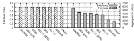
We also see that MadMac has the better global throughput among the fair MAC protocols. This throughput is the maximum throughput that can be achieved under a Max-Min fairness restriction. This maximum throughput is achieved with MadMac by synchronizing the 3 pairs by using carrier sensing information. In SBA, we do not use such a synchronization scheme and we can see that the performance of SBA is smaller but not so far from the fair capacity. We can also notice that SBA is more efficient than MBFAIR and PNAV. The hidden terminals Figure 3 shows the fairness index and the global through-put obtained in the hidden terminals scenario presented in Figure 1(a). As the stations have a symmetrical behaviour, the two stations have statistically the same behaviour (see [11] for more details). Thus, there is no long term unfairness issue with this scenario, as the different fairness indexes show. We can see from this figure that, when SBA is randomly asynchronous, the global throughput is roughly the same as with 802.11. But when the stations are fully synchronized, the global throughput of SBA is better than the throughput of 802.11 with or without the use of RTS/CTS mechanisms. The throughput of MadMac is better than the throughput of SBA, because MadMac synchronizes the hidden terminal by using the acknowledgement to identify the hidden terminals problem. Note that the performance of MadMac degrades when acknowledgements are not used. We show here that SBA can provide a good fairness-efficiency trade-off without any information. 0 0.2 0.4 0.6 0.8 1 1.2
MadMacSBA syncDIDD 802.11 (RTS)SBA 802.11MBFAIRPNAV MadMacSBA syncDIDD 802.11 (RTS)SBA 802.11MBFAIRPNAV 0
1000 2000 3000 4000 5000 6000 7000 Fairness Index Aggregate th. (kbps) Efficiency Fairness
Fig. 3.Simulation results for the hidden terminals scenario.
The asymmetric hidden terminals Figure 4 shows the simulation results on the asymmetric hidden terminals, given in Figure 1(b). We can see that when the stations are synchronized, the throughput of SBA is close to the throughput of 802.11 and the fairness index of SBA is close to 1, which means that the two emitters have roughly the same throughput. The figure also shows that even if the stations are not synchronized, the performances of SBA are either better or close to the performances of the other fair protocols. These good performances are due to the alternation between the use of the contention window sizes. Concerning
802.11 (or DIDD), it is more efficient than all the other tested protocols, but much less fair.
0 0.2 0.4 0.6 0.8 1 1.2
SBA syncMBFAIRSBA MadMacPNAV 802.11 (RTS)802.11DIDD SBA syncMBFAIRSBA MadMacPNAV 802.11 (RTS)802.11DIDD 0
1000 2000 3000 4000 5000 6000 7000 Fairness Index Aggregate th. (kbps) Efficiency Fairness
Fig. 4.Simulation results for the asymmetric hidden terminals scenario.
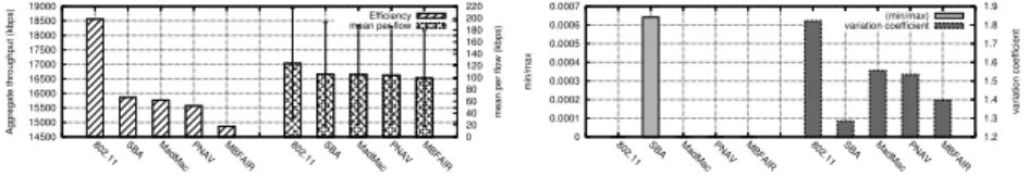
Random topologies In this subsection, we present the results on random topologies. In these topologies, stations’ positions are uniformly and randomly chosen in a square of 500m × 500m size. The communication range of the station is set to 150m. Sources and destinations of flows are also randomly chosen. It is worth noting that, in these simulations, the same topology and flows config-uration are tested for each protocol. The results given in this section are thus topology dependent.
Due to the random aspect of these scenarios, the performance metrics we use are different. For efficiency, we compute the global throughput of the network, the mean throughput of each flow and the corresponding 95% confidence interval. For fairness, we measure the min−max ratio which is the ratio between the minimum throughput achieved in the network over the maximum throughput. This metric has the advantage, compared to the usual variance, of being independent from the number of considered emitters and does not mask the situation in which a few stations are starved. If the min − max ratio is close to 1 this means that all emitters have the same throughput. If the min − max ratio is equal to 0, it means that at least one flow is starved in the networks. We also use the variation coefficient which gives the dispersion around the mean value. The variation coefficient is the ratio of the standard deviation over the mean. This metric is independent from the mean value unlike the usual variance. The higher the value of the coefficient, the higher the dispersion around the mean value. This metric gives an intuition on how the flows are distributed around the mean value.
14500 15000 15500 16000 16500 17000 17500 18000 18500 19000
802.11 SBA MadMac PNAV MBFAIR 802.11SBA MadMac PNAV MBFAIR 0
20 40 60 80 100 120 140 160 180 200 220 Aggregate throughput (kbps)
mean per flow (kbps)
Efficiency mean per flow
0 0.0001 0.0002 0.0003 0.0004 0.0005 0.0006 0.0007
802.11SBA MadMac PNAV MBFAIR 802.11SBA MadMac PNAV MBFAIR 1.2
1.3 1.4 1.5 1.6 1.7 1.8 1.9 min/max variation coefficient (min/max) variation coefficient
Figure 5 shows the simulations results in a random scenario with 200 stations and 150 flows. This figure shows that SBA is slightly more efficient than MadMac, PNAV and MBFAIR. We can also see that no flow is starved with SBA, unlike the other protocols for which the min − max ratio is equal to 0. The coefficient variation also shows that the dispersion around the mean throughput is smaller for SBA, which means that the flows’ throughputs are close. This figure shows that in this case, SBA is the best trade-off between fairness and efficiency. To better see the difference between SBA and the other protocols, we plotted the distribution of the flows throughputs.
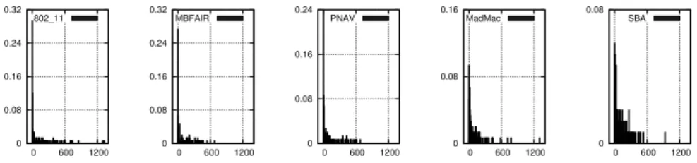
0 0.08 0.16 0.24 0.32 0 600 1200 802_11 0 0.08 0.16 0.24 0.32 0 600 1200 MBFAIR 0 0.08 0.16 0.24 0 600 1200 PNAV 0 0.08 0.16 0 600 1200 MadMac 0 0.08 0 600 1200 SBA
Fig. 6.Throughputs distribution for a random scenario with 200 stations and 150 flows (throughput vs percentage of flows achieving this throughput).
Figure 6 shows the throughputs distribution of each protocol. The x-axis gives the throughput in kbps and the y-axis the proportion of flows that get this throughput. The size of each chart is equal to 3 kbps. We can see that with SBA, the number of flows that have a throughput close between 0 and 3 kpbs is less than 6%. Moreover, the min − max ratio tells us that no flow is starved with SBA. On the other hand, with 802.11, more than 28% of flows have a throughput between 0 and 3 kpbs. This value is more than 24% for PNAV and MBFAIR and more than 8% for MadMac. These charts also show that the difference between the aggregated throughputs of 802.11 and SBA comes from the fact that with 802.11 a little proportion of flows can get more that 1200 kbps. With SBA, there is no flow with such a throughput, the higher throughput is around 920 Kbps. One interesting point is that even if a small percentage of flows have a throughput around 1300 Kbps with MadMac, the global throughput of MadMac is lower than the SBA’s one.
It is worth noting that we ran many other random simulations and the results are always the same. We mean here that SBA exhibits a good trade-off between fairness and efficiency among the tested protocols.
5
Complexity
The complexity of MAC protocols for ad hoc networks is hard to quantify. In this section, we define some parameters to quantify complexity and then we provide the measure of each indicator for the protocols we compare in the previous section.
5.1 Complexity parameters
(HD) History dependence: with this parameter, we try to provide the age of the information used by each protocol.
(Dist) Distance of information given in number of hops: it indicates the locality degree of the protocol.
(E) Event: it indicates the event(s) from which the protocol reacts. We have identified different events: (a) successful transmission and/or collision: such an event gives, to a node, the status of the packet it has just sent; (b) carrier sensing detection; (c) reception of control packets: the protocol can use control packets to adapt its behavior; (d) reception of data packets from which the protocol can extract and use useful information like packet source, packet size, etc.
(NV) Number of variables: we give here the maximum number of variables that are modified by a node after each different event given previously and used by the protocol.
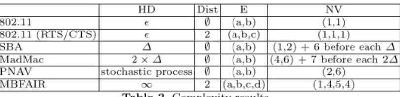
5.2 Complexity results
Table 2 gives the complexity parameters for the MAC protocols we evaluate in Section 4. For the HD parameter, ǫ means that the history length is very short, i.e. the protocol adapts its behavior just after an event. For example, IEEE 802.11 DCF only needs the transmission status of the last sent packet. Stochastic process means that the history length depends on a stochastic process which can be probabilistically long even if it can only depend on the previous status of the protocol.
We give the NV parameter in respect to the format of the parameter (E): for
instance (xa, xb) for NV corresponds to at most xamodified variables after event
(a) and xbmodified variables after event (b) if E is denoted by (a,b). With 802.11,
each node stops its backoff decrease after event (a) or changes its contention window size or not after event (b). When RTS/CTS are activated, these packets are also used to update the NAV, which corresponds to one variable modification
after event (c). With SBA, Tsucc or Tcol and Nsucc or Ncol are updated after
event (b). At the end of each interval, the four different probabilities, as the new contention window size, are computed, and ∆ is reset. This is denoted by 6 before each ∆ in the table. With MadMac, more variables are maintained and modified: after event (a), the backoff decrease is stopped, but some variables are updated to indicate the share of the medium as the status of a possible multiple hidden nodes configuration; after event (b), the contention window size may be updated, but MadMac also counts, via some variables, the number of collisions as the number of successive sent packets and infers, via other variables, whether the node is within a multiple hidden nodes configuration. At the end of the ∆ period, some of these variables are reset. With PNAV, a stochastic process is used to determine if the NAV is used or not. For that, different variables are updated after events (a,b). With MBFAIR, four variables are updated after event (b), (c) or (d): thanks to the sent packets or the received packtets, each node can compute its medium’s occupancy of the medium, the medium’s occupancy of
the other stations, its fair share and the contention window size to use. With the receipt of RTS/CTS, each node can also update its NAV.
HD Dist E NV
802.11 ǫ ∅ (a,b) (1,1)
802.11 (RTS/CTS) ǫ 2 (a,b,c) (1,1,1)
SBA ∆ ∅ (a,b) (1,2) + 6 before each ∆
MadMac 2 × ∆ ∅ (a,b) (4,6) + 7 before each 2∆
PNAV stochastic process ∅ (a,b) (2,6)
MBFAIR ∞ 2 (a,b,c,d) (1,4,5,4)
Table 2.Complexity results.
It is difficult to order these algorithms in terms of complexity. It is clear the IEEE 802.11 without RTS/CTS uses very few information and very few variables. If we consider that the use of control packets introduces more complexity in the protocol than local operations, then SBA is rather simple and requires less variables than MadMac.
6
Conclusion and future works
In this paper, we have presented a new backoff algorithm for ad hoc networks: only two contention window sizes are used and the choice of the contention window depends on computations based on local information only. Compared to existing backoff algorithms, SBA is designed for ad hoc networks. The results presented in this paper show that SBA is fairer than 802.11. Of course, the fairness induced by SBA reduces the global throughput (compared to 802.11), but this decrease is often lower than the one achieved by some other fair MAC protocols. Given the first obtained results, we think that SBA is a good candidate in terms of trade-off between fairness, simplicity and efficiency.
The next step of this work is to modify the value of each parameter of SBA
such as CWmin, CWmax and the conditions presented in the algorithm to
opti-mize the performances of SBA depending on the requirement of the networks.
References
1. IEEE, between Systems, I.E.: Local and Metropolitan Area Network – Specific Re-quirements –Part 11: Wireless LAN Medium Access Control (MAC) and Physical Layer (PHY) Specifications. The Institute of Electrical and Electronics Engineers (1997)
2. Chaudet, C., Dhoutaut, D., Gu´erin-Lassous, I.: Performance Issues with IEEE 802.11 in Ad Hoc Networking. IEEE Communications Magazine 43(7) (July 2005) 110–116
3. Bharghavan, V., Demers, A., Shenker, S., Zhang, L.: MACAW: a media access pro-tocol for wireless LAN’s. In: ACM SIGCOMM Computer Communication Review, London, United Kingdom (1994) 212–225
4. Chatzimisios, P., Boucouvalas, A., Vitsas, V., Vafiadis, A., Oikonomidis, A., Huang, P.: A simple and effective backoff scheme for the IEEE 802.11 MAC protocol. In: Cybernetics and Information Technologies, Systems and Applications (CITSA), Orlando, Florida, USA (July 2005)
5. Fang, Z., Bensaou, B., Wang, Y.: Performance evaluation of a fair backoff algorithm for IEEE 802.11 DFWMAC. In: ACM Symposium on Mobile Ad Hoc Networking and Computing (MOBIHOC), Lausanne, Switzerland (2002) 48–57
6. Nandagopal, T., Kim, T., Gao, X., Bharghavan, V.: Achieving MAC Layer Fairness in Wireless Packet Networks. In: ACM Conference on Mobile Computing and Networking (MOBICOM), Boston, Massachusetts, United States (2000) 87–98 7. Luo, H., Lu, S., Bharghavan, V.: A new model for packet scheduling in multihop
wireless networks. In: ACM Conference on Mobile Computing and Networking (MOBICOM), Boston, Massachusetts, United States (2000) 76–86
8. He, J., Pung, H.K.: Fairness of Medium Access Control Protocols for Multi-hop Ad Hoc Wireless Networks. Computer Networks 48(6) (2005) 867–890
9. Chaudet, C., Chelius, G., Meunier, H., Simplot-Ryl, D.: Adaptive Probabilistic NAV to Increase Fairness in Ad Hoc 802.11 MAC. Ad Hoc and Sensor Wireless Networks: an International Journal (AHSWN) 2(2) (June 2005)
10. Razafindralambo, T., Gu´erin-Lassous, I.: Increasing Fairness and Efficiency using the MadMac Protocol in Ad Hoc Networks. Ad Hoc Networks Journal, Elsevier Ed. 6(3) (May 2008) 408–423
11. Li, Z., Nandi, S., Gupta, A.K.: Modeling the Short-Term Unfairness of IEEE 802.11 in Presence of Hidden Terminals. In: IFIP NETWORKING. (2004) 613–625 12. Dhoutaut, D., Gu´erin Lassous, I.: Impact of Heavy Traffic Beyond
Communi-cation Range in Multi-Hops Ad Hoc Networks. In: Third International Network Conference, Plymouth, Angleterre (2002)
13. NS-2: The Network Simulator. http://www.isi.edu/nsnam/ns/
14. Jain, R., Durresi, A., G., B.: Throughput Fairness Index: An Explanation. In: ATM Forum Document Number: ATM Forum/990045. (February 1999)