Lire la première partie de la thèse

(1)

la

première partie

de la thèse

(2)

Physics and modelling around two

supercritical airfoils

3.1 Shock-vortex shear-layer interaction in

tran-sonic buffet conditions

The OAT15A is a supercritical airfoil designed by ONERA (Jacquin et al., 2005) in the context of the ATAAC European project (same as the tandem of cylinders, chapt. 2). The numerical aspects of the simulations of this test case, as well as some physical properties, in transonic buﬀet conditions, have been investigated by Fernando Grossi in our research team in the context of a Master’s and a Ph.D. theses (Grossi, 2010, 2014) and have been published in articles (Grossi et al., 2014) as well as proceedings from several oral communications (Grossi et al., 2011,2012b,a). Enriched from all this work, new simulations have been performed and the physics of

(3)

results on the physical analysis, have been the subject of an article accepted in the Journal of Fluids and Structures in March 2015Szubert et al. (2015b). This article is fully reproduced in this manuscript in the following section to present the results, in addition to details about the geometry and the numerical method. A discussion about the upscale turbulence modelling, in the context of the ensemble-averaged approaches, is given in section 3.1.2.

3.1.1 Shock-vortex shear-layer interaction in the transonic

flow around a supercritical airfoil at high Reynolds

number in buffet conditions

(4)

Shock-vortex shear-layer interaction in the transonic flow around a supercritical airfoil at high Reynolds number in buffet conditions

Damien Szuberta,n

, Fernando Grossia_{, Antonio Jimenez Garcia}a_,

Yannick Hoaraub_{, Julian C.R. Hunt}c_{, Marianna Braza}a

a_{Institut de Mécanique des Fluides de Toulouse, UMR No 5502 CNRS-INPT-UPS, Allée du Prof. Camille Soula, F-31400 Toulouse, France} b_{Laboratoire ICUBE, UMR No 7357, Strasbourg, France}

c_{Department of Earth Sciences, University College London, London WC1E 6BT, UK}

a r t i c l e i n f o

Article history:

Received 4 April 2014 Accepted 7 March 2015 Available online 2 May 2015

Keywords: Transonic flow Buffet instabilities Wavelets POD Turbulence modelling Stochastic forcing a b s t r a c t

This paper provides a conceptual analysis and a computational model for how the unsteady ‘buffeting’ phenomenon develops in transonic, low incidence flow around a supercritical aerofoil, the OAT15A, at Reynolds number of 3.3 million. It is shown how a low-frequency buffet mode is amplified in the shock-wave region and then develops upstream and downstream interaction with the alternating von Kármán eddies in the wake past the trailing-edge as well as with the shear-layer, Kelvin–Helmholtz vortices. These interactions are tracked by wavelet analysis, autoregressive (AR) modelling and by Proper Orthogonal Decomposition. The frequency modulation of the trailing-edge instability modes is shown in the spectra and in the wall-pressure fluctuations. The amplitude modulation of the buffet and von Kármán modes has been also quantified by POD analysis. The thinning of the shear layers, both at the outer edge of the turbulent boundary layers and the wake, caused by an ‘eddy-blocking’ mechanism is modelled by stochastic forcing of the turbulent kinetic energy and dissipation, by small-scale straining of the higher-order POD modes. The benefits from thinning the shear-layers by taking into account the interfacial dynamics are clearly shown in the velocity profiles, and wall pressure distribution in comparison with the experimental data.

1. Introduction

Understanding the various mechanisms related to buffet instabilities in the transonic flow around a supercritical airfoil is the main objective of this paper. A detailed physical analysis is developed for the interactions between shock waves and the boundary layer over the aerofoil, as well as between wake vortices and the shock waves. A further complexity arises from the interactions between the wake vortices near the trailing edge and the fluctuating sheared interface that bounds the wake flow.

Pioneering studies ofLevy (1978)andSeegmiller et al. (1978), made evidence of a shock unsteadiness characterised by a

low-frequency and high-amplitude, in the Mach number range 0.7–0.8 corresponding to aircraft's cruise-speed. Several experimental

Contents lists available atScienceDirect

journal homepage:www.elsevier.com/locate/jfs

Journal of Fluids and Structures

n_{Corresponding author.}

(5)

and numerical studies have been devoted to this flow phenomenon and its impact on the aerodynamic forces:McDevitt et al. (1976),Jacquin et al. (2005,2009) andBrunet (2003).

Whereas the majority of the studies devoted to the transonic interaction deal with the high-Reynolds number range, the physical mechanisms of the buffet onset can be studied more easily in the lower Reynolds number range, allowing for Direct

Numerical Simulation. For a NACA0012 airfoil, (Bouhadji and Braza, 2003a,2003b) have analysed the successive states of the

unsteadiness due to the compressibility effects in the Mach number range 0.3–1.0 by 2D and 3D Navier–Stokes simulations. The buffet instability was analysed in association with the von Kármán vortex shedding in the Mach number range 0.75– 0.85, as well as the suppression of the buffet form Mach numbers beyond 0.85. The buffet mode has also been analysed by

DNS ofBourdet et al. (2003), who used in addition the Stuart-Landau model (Landau, 1944) in order to quantify the linear

and non-linear parts of the buffet instability.

These studies showed the sharp rise of the drag coefficient as the Mach number increases in the range 0.7–0.8, as well as the interaction of the shock wave with the von Kármán wake instability downstream of the trailing-edge. It was shown that this instability was formed in the wake and propagated towards the trailing-edge beyond a low-subsonic critical value of the

Mach number, of order 0.2, for a NACA0012 airfoil at zero incidence and Reynolds number of 10 000 (Bouhadji, 1998). This

instability (mode I) persists within the whole transonic speed interval, up to Mach number of order 0.85, independently on the appearance of the buffet. This second instability (mode II) was found to appear in the interval 0.75–0.8 and to strongly interact with mode I, where the buffet was sustained by mode I. Experimental evidence of mode I was made by the

Schlieren visualisations of D.W. Holder (Fung, 2002),Fig. 7.

Numerical simulations in the high-Re range (Grossi et al., 2012b;Jimenez-Garcia, 2012), regarding a supercritical airfoil,

the OAT15A, introduced a splitter-plate at the trailing edge, which suppressed the von Kármán mode. It was shown that in the cases where the von Kármán mode was remote (downstream of a critical length of the splitter plate), the buffet mode was considerably attenuated and disappeared. Therefore, it is worthwhile analysing the interaction of these two modes in the high-Reynolds number regimes for aerodynamics applications. In particular, there is little knowledge of this kind of interaction in the state of the art with regard to the high-Re range as well as more generally, of the trailing-edge dynamics

feedback effect towards the shock-wave/boundary-layer interaction region (SWBLI) upstream of the trailing-edge. Lee

(1990)reported a schematic explanation of the buffet interaction with Kutta waves coming from the trailing-edge, without a quantification of this interaction. Furthermore, it is worthwhile mentioning that the SWBLI is followed by separation of the boundary layer and by the formation of thin shear layers at the edges of the boundary layers and in the wake, where local Kelvin–Helmholtz (K–H) instabilities are observed.

In order to compute the interactions and feedback between the shear-layer and trailing-edge instabilities with the upwind shock-buffet mode, new methods are needed. These have to overcome the tendency of the shear layers to thicken downstream of the SWBLI, because of the turbulent shear stress modelling near the interface is usually approximated by employing eddy-viscosity concepts based on equilibrium turbulence hypotheses and direct cascade. In the flow physics however, upscale phenomena occur that increase the energy of the turbulence spectrum from intermediate range towards

the lower wavenumbers (Braza et al., 2006). These mechanisms are not yet sufficiently taken into account in the modelling

equations. However, theoretical analysis (Hunt et al., 2008) and experimental studies (e.g.Ishihara et al., 2015) show that

these stresses are generated by the inhomogeneous small-scale motions in the turbulent region near the interface and

thence increase the local “conditional” shear and “eddy blocking effect” within the interfacial layer (Fig. 1). This influence of

small scales on the whole flow is effectively an “upscale” process. The local turbulence adjacent to the interface tends to

reduce the Kelvin–Helmholtz instability modes of the interface (Dritschel et al., 1991).

A new approach for modelling the interface regions is needed, which can be based on recent numerical and experimental research into turbulent interfacial shear flows, on the outer edges of jets, wakes and the outer parts of boundary layers with thickness L. The thin randomly moving interfaces which separate regions of strong and weak turbulence have a thickness

ℓ_{(≪L). This general property of turbulent flows was in fact suggested and discussed by Prandtl in 1905, though he did not}

take it further once he became interested in the mixing length model of the mean properties of turbulent shear flows (see

Bodenschatz and Eckert, 2011;Taveira and da Silva, 2014). Within these layers, the average shear (or in 2-dimensions the gradient of shear) is much stronger than that in the adjacent turbulent shear flows. At very high Reynolds numbers Re,

determined by L and the R:M:S:, turbulent velocity uo, the thickness ℓ of these interface layers is of the order of the Taylor

microscale ℓv(i.e L Re! 1=2), but within them very thin elongated vortices form with a thickness ℓvof the order of the

Kolmogorov microscale (i.e. ℓv" L Re! 3=4,Eames and Flor, 2011). Numerical simulations show that these sharp interfaces

occur even in complex turbulent flows, such as flows over aircraft wings (Braza, 2011).

These interfaces have their own mean local dynamics that keep the mean gradients at the interface at a maximum,

through eddy blocking and enhanced vortex stretching (Hunt et al., 2008). Similar bounding interfaces also occur at the

edges of patches of turbulence, such as puffs or vortex rings (Holzner et al., 2008). These intensely sheared layers interact

with the motions outside the layers by blocking external eddies (through shear sheltering), which leads to a balance

between sharpening of the velocity gradients in the layer and the tendency to diffuse outwards (Hunt et al., 2008). The

typical spacing between the interfacial layers is of order of the “dissipation integral length scale” (Hunt et al., 2014).

Thus, the overall high-Re dynamics of the interface has to be modelled in order to correctly represent the turbulent transfers through the rotational–irrotational regions either side of these interfaces that have to be kept thin. This modelling has to include the complex interactions between the developing instability modes and the fine-scale turbulence. It is necessary to have a comprehensive turbulence model that should include the effects of the low-frequency organized motion

(6)

and the transfers due to the random turbulence. Such models should take sufficient account of the large and small motion

effects, especially the shear–stress gradients as studied at high-Re atmospheric flows byHunt et al. (1984). The turbulence

modelling in the present case should also accurately predict the pressure distribution and the unsteady loads in fluid– structure interaction.

In this context, approaches such as standard URANS, derived from assumptions of turbulence in statistical equilibrium and using downscale cascade, tend to produce higher rates of the turbulence kinetic energy and to underestimate the global

coefficients (drag, lift) and their amplitudes (Haase et al., 2009).

The Large Eddy Simulation uses a number of degrees of freedom being orders of magnitude higher than the grid size needed

for URANS and hybrid approaches. For moderate Reynolds number flows (Re Oð104

Þ), LES can capture the major instabilities past

bodies, whereas for the high-Reynolds number range (Re 4106), for industrial designs, it is not practical with typical

computational capacity to apply LES for aerodynamic flows around lifting structures. Furthermore, even with LES methods, improvements can be expected by reconsidering the classical downscale energy transfer models for the small-scale eddies in the dissipative wave-number range by using upscale transfer processes in the turbulence modelling of the thin interfaces.

Recent efforts in turbulence modelling are devoted to accurately reproduce the flow physics in respect of instability amplification, strong flow detachment and accurate prediction of the associated frequencies, unsteady loads and in particular, of pressure fluctuations, representing a crucial need for aeroacoustics.

Hybrid RANS-LES methods are quite suitable for this category of fluid–structure interaction problems, because they associate the benefits of URANS in the near-region and those of LES in the regions of flow detachment, as reported the

proceedings of the 4th HRLM, ‘Hybrid RANS-LES Methods’ symposium (Fu et al., 2012). Hybrid methods can be considerably

improved by using adapted URANS modelling in the near-wall region and adapted LES modelling in the flow detachment areas, in order to allow for modification of the turbulent scales accounting for non-equilibrium turbulence.

In this context, improved URANS approaches can be used to reduce the turbulent viscosity levels and allow the

amplification of instabilities, as for example the Scale Adaptive Simulation (SAS;Menter and Kuntz, 2003;Menter and

Egorov, 2005), the Organised Eddy Simulation (OES;Braza et al., 2006;Bourguet et al., 2008, among others). SAS adapts the Kolmogorov turbulence scale according to flow regions governed by non-equilibrium turbulence effects. OES accounts for stress-strain directional misalignment in non-equilibrium turbulence regions thanks to a tensorial eddy-viscosity concept derived from Differential Reynolds Stress Modelling (DRSM) projection on the principal directions of the strain-rate tensor. Although significant conceptual progress has been accomplished in the last decade, there still remain open questions with regard to the quantitative prediction of the above mechanisms with the accuracy required by the design. To our knowledge, the majority of the available modelling approaches produce less thin shear-layer interfaces, even by using considerably fine grids. This is generally due to a higher turbulence diffusion level than in the physical reality, produced by the modelling approaches, which mostly employ downstream turbulence cascade assumptions. In the present paper, the motivation is to enhance the eddy-blocking effect and vortex stretching in the sense of an upscale cascade.

On view of the above elements, the objectives of the present paper are as follows: to analyse in detail the interaction between two main instabilities, the buffet and the von Kármán modes in the transonic flow around a supercritical airfoil, whose configuration is involved in the next generation of civil aircraft design, by means of numerical simulation and adapted turbulence modelling concepts. A method of stochastic, inhomogeneous forcing of the turbulence transport equations is presented. This models the thin turbulent/non-turbulent, shear-layer interfaces and thence the large-scale flow structure on the purpose to provide the correct pressure fluctuations needed for fluid–structure interaction. The content of

the following sections are as follows:Section 2presents the flow configuration and the numerical approach.Section 3

presents the results regarding the buffet instability, its interaction with the shear-layer and near-wake instabilities based on conventional URANS/OES methods. This section includes in particular wavelet analysis and Proper Orthogonal

Decomposi-tion. InSection 4, the stochastic forcing approach for the higher modes is presented and compared with other methods and

experimental results.Section 5is the conclusion of the paper.

2. Flow conﬁguration, numerical method and turbulence modelling

2.1. Test case description

The transonic buffet over the OAT15A airfoil was investigated in the experimental work byJacquin et al. (2005,2009), as

well as byBrunet et al. (2003), by means of both experimental and numerical study at free-stream Mach numbers in the

range of 0.70–0.75 and a chord-based Reynolds number of 3 million. The OAT15A is a supercritical wing section with a thickness-to-chord ratio of 12.3%. The wind tunnel model has a chord of C¼0.23 m and a blunt trailing edge measuring 0.005C. The airfoil was mounted wall-to-wall and the boundary layer was tripped on both sides at x=C ¼ 0:07 from the leading edge for fully-turbulent behavior. The results showed that a periodic self-sustained shock-wave motion (buffet) was obtained for angle of attack values higher or equal to 3.51. A detailed experimental study, for this angle of attack, is reported in Jacquin et al. (2009). The main flow features concerning buffet were essentially two dimensional, and the buffet

D. Szubert et al. / Journal of Fluids and Structures 55 (2015) 276–302

(7)

2.2. Numerical method

The simulations of the OAT15A configuration have been carried out with the Navier–Stokes Multi-Block (NSMB) solver. The NSMB solver is the fruit of a European consortium that included Airbus from the beginning of '90s, as well as main European aeronautics research Institutes, as KTH, EPFL, IMFT, ICUBE, CERFACS, Univ. of Karlsruhe, ETH-Ecole Polytechnique de Zurich, among other. This consortium is coordinated by CFS Engineering in Lausanne, Switzerland. NSMB is a structured code that includes a variety of efficient high-order numerical schemes and of turbulence modelling closures in the context of

LES, URANS and of hybrid turbulence modelling. A first reference of the code description can be found inVos et al. (1998)

concerning the versions of this code in the decade of '90s. Since then, NSMB highly evolved up to now and includes an ensemble of the most efficient CFD methods, as well as adapted fluid–structure coupling for moving and deformable

structures. These developments can be found inHoarau (2002)regarding URANS modelling for strongly detached flows,

Martinat et al. (2008), in the area of moving body configurations,Barbut et al. (2010)andGrossi et al. (2014)allowing for Detached Eddy Simulation with the NSMB code.

NSMB solves the compressible Navier–Stokes equations using a finite-volume formulation on multi-block structured grids. In 3D cartesian coordinates ðx; y; zÞ, the unsteady compressible Navier–Stokes equations can be expressed in conservative form as

∂ ∂tð ÞþW ∂ ∂xðf !fvÞþ ∂ ∂yg !gv ! " þ_∂∂_zðh !hvÞ ¼ 0; ð1Þ

where t denotes the time. The state vector W and the inviscid fluxes f, g and h are given in the following for the laminar model:

W ¼ ρ ρU ρV ρW ρE 0 B B B B B B @ 1 C C C C C C A ; f ¼ ρU ρU2þp ρUV ρUW UðρE þpÞ 0 B B B B B B @ 1 C C C C C C A ; g ¼ ρV ρVU ρV2þp ρVW VðρE þpÞ 0 B B B B B B @ 1 C C C C C C A ; h ¼ ρW ρWU ρWV ρW2 þp WðρE þpÞ 0 B B B B B B @ 1 C C C C C C A : ð2Þ

Fig. 1.Schematic diagram of shock, shear-layer and wake dynamics, including SWBLI, showing how the shear layer of the interface remains thin as a result of eddy-blocking mechanism.

Fig. 2.Comparison of spectra of pressure signal for 2 different time steps; left: Δt ¼ 10! 6_{s; right: Δt ¼ 0:5 ' 10}! 6_s.

(8)

Hereρis the density, U, V and W are the cartesian instantaneous velocity components, p is the pressure and E is the total energy. The viscous fluxes are defined as

fv¼ 0 τxx τxy τxz τU ð Þx!qx 0 B B B B B B @ 1 C C C C C C A ; gv¼ 0 τyx τyy τyz τU ð Þy!qy 0 B B B B B B @ 1 C C C C C C A ; hv¼ 0 τzx τzy τzz τU ð Þz!qz 0 B B B B B B @ 1 C C C C C C A ; ð3Þ

whereτijare the components of the stress tensor, qithe heat flux (Fourier's law) and the work due to the viscous dissipation is

expressed asðτUÞi¼τixU þτiyV þτizW.

The third-order of accuracy Roe upwind scheme (Roe, 1981) associated with the MUSCL van Leer flux limiter scheme (van

Leer, 1979) is used to discretize the convective fluxes. Implicit time integration using the dual time stepping technique with

3 Gauss–Seidel iterations has been performed. A physical time step of 0:5μs has been adopted ( ( 5 ' 10! 4_C=U

1) after

detailed tests carried out inGrossi (2010).

A study of the time step has been carried out with the grid used in this study. The Power Spectral Density (PSD) of the

pressure signal on the airfoil at the location x=C ¼ 0:45 for two time steps are shown inFig. 2. The PSD spectrum on the left

has been obtained from a calculation with a time step Δt ¼ 10! 6_{s, while the spectrum on the right comes from a}

calculation with a time step twice smaller and used in this study. A very similar distribution of the PSD can be observed in terms of frequency as well as of the energy level. A typical number of 30 inner iterations was necessary for the convergence

in each time step. The convergence criterion at the inner step n is defined by the ratio between the L2-norm of the density

equation residual at the inner step n and the one at the initial inner step. The methodology adopted in the simulations is the

same as inGrossi et al. (2014).

The grid has a C–H topology. Two different grids had been compared in previous studies (Grossi, 2014). The first is of size

110 000 cells approximately, used byDeck (2005)and provided within the partnership in the ATAAC (Advanced Turbulence

Simulations for Aerodynamic Application Challengers) European program No. 233710 and a second, finer grid built in our

research group, having 130,000 cells and a domain size of 80 chords. A comparison of these two grids is provided inFig. 3.

The mean value of the pressure coefficient (Fig. 3left) and the RMS pressure distribution over the airfoil (Fig. 3right) are

very similar for the two grids. The buffet frequency is practically unchanged. The second grid has been used for the present

Fig. 3.Grid comparison concerning the mean wall-pressure coefficient (left) and the normalized RMS of the pressure fluctuations (right); experiment by Jacquin et al. (2009).

(9)

study. The yþ_{coordinate regarding the turbulence modelling near the wall is smaller than 0.5 in the whole domain.}_{Fig. 4}

shows the grid and the computational domain.

2.2.1. Boundary conditions

On the solid wall, impermeability and no-slip conditions are employed. The far-field conditions are characteristic

variables with extrapolation in time, defined by means of the experimental upstream values, the total pressure (P0¼ 105Pa)

and total temperature (T0¼ 300 K), as well as the upstream Reynolds number of 3 million. The upstream turbulence

intensity is set equal to the experimental value of Tu¼1%.

2.3. Turbulence modelling

Based on previous studies in our research group which examined the predictive ability of various turbulence models (Grossi et al., 2011,2012a;Grossi, 2014), it was shown that the two-equation k!ω-SST model (Menter, 1994) was not able to

produce any unsteadiness at the present incidence value. The Spalart-Almaras model (SA;Spalart and Allmaras, 1994) in its

standard version, and its Edwards and Chandra variant (SA-E;Edwards and Chandra, 1996) with compressibility correction

of Secundov (SA-EþCC;Shur et al., 1995;Spalart, 2000), underpredicted the amplitudes of the shock motion, even by

tripping the flow at x=C ¼ 0:07 like in the experiment (trip), which does not have a significant effect on the flow. The strain

adaptive formulation of the Spalart–Allmaras model (SALSA;Rung et al., 2003) gave good amplitudes but no secondary

oscillations. The k!ε-OES model (Braza et al., 2006;Bourguet et al., 2008) involving in the present study an eddy-diffusion

coefficient Cμ¼ 0:03, was able to produce the shock unsteadiness with a frequency close to the experimental one. Moreover,

Fig. 5.Comparison of the time-dependent evolution of the lift coefficient between the strain adaptive formulation of the Spalart–Allmaras model (SALSA), the Edwards and Chandra variant of the Spalart–Allmaras model using compressibility corrections (SA-EþCC) without and with tripping at x=C ¼ 0:07 (trip) and the k!ε-OES modelling.

Time (s) 0 0.005 0.01 0.015 0.02 0.025 0.03 0.035 -7 -6.5 -6 -5.5 -5 -4.5 -4 -3.5 EXP SALSA SA-E+CC k- OES

Fig. 6.Comparison of the time-dependent evolution of the surface pressure at x=C ¼ 0:45 between three turbulence models as inFig. 5; experiment by Jacquin et al. (2009).

(10)

the formation of secondary oscillations within the buffet cycles, mainly due to intermittent von Kármán vortex shedding,

has been captured. These results can be observed inFig. 5for the evolution of the lift coefficient and in Fig. 6for the

evolution of the pressure versus time at x=C ¼ 0:45. The latter is compared with the experimental results fromJacquin et al.

(2009)where the secondary oscillations are visible both in experiment and in the simulation with the k!ε-OES model.

3. Results

3.1. Buffet phenomenon and trailing-edge instabilities

According to the OES method, the resolved turbulence corresponds to an ensemble-averaged flow evolution, representing the organised, coherent part of the flow. A first overview of the buffet phenomenon and of the shear-layer

and trailing-edge instabilities is represented inFig. 8, by means of the velocity divergence field (∇ * U ¼ ∂xU þ∂yV þ∂zW),

which highlights compressibility effects around the airfoil and illustrates density gradients similar to the Schlieren visualizations. A qualitative similarity of the physical phenomena (shock waves, shock foot, wake) observed in the Schlieren

visualization, for the experiment, by D.W. Holder (Fung, 2002; Fig.7), and the field of divergence of velocity, for the CFD, is

provided by the figures.

In the present study, the dimensionless time is tn

¼ tU1=C. Furthermore, tn¼ 0 was set to the maximum lift phase, with

the shock wave at its most downstream position, as illustrated inFig. 8(a). At that moment, in addition to the separation

bubble at the foot of the shock, rear separation is also developed. These two regions grow simultaneously and fuse into a large separation area extending from the foot of the shock to the trailing edge. This scenario coincides with the well

developed shock-wave motion towards the upstream direction, represented inFig. 8(b). This figure shows the presence of a

von Kármán instability, which quickly gives rise to alternate vortex shedding. In addition, Kutta-type waves are generated at the trailing edge of the airfoil and move upstream, at both sides of the airfoil. Upside, waves are refracted by the shock wave (Fig. 8(e)). As the shock moves towards the leading edge, the thickness of the separated region increases progressively, causing a dramatic decrease of the lift coefficient. As the shock wave comes towards its most upstream positions, the

boundary layers becomes more and more detached. At the most upstream position (Fig. 8(f)), the reattachment process

starts and reaches full reattachment while the shock is moving downstream (Fig. 8(g)), until x=C ¼ 0:60 approximately

(Fig. 8(h)). The alternate vortex shedding practically disappears, and the trailing-edge waves generation is temporarily attenuated, until the shear layer thickens again for a new cycle of buffeting.

The transonic flow around the symmetric NACA0012 airfoil (Bouhadji and Braza, 2003b), where a shock wave is observed

on both upper and lower sides of the body, is cited in the introduction in order to comment the interaction between the buffet and the von Kármán modes. In the buffet regime (M¼0.80), the boundary layers downstream of the shock waves are alternately separated, inducing a thicker effective obstacle between the two separated shear layers that generates significant vorticity gradients in the trailing-edge region and hence creates the von Kármán mode. In the case of the supercritical OAT15A airfoil, at a slight angle of attack (3.5–3.91), only one supersonic region exists at the upper side. In the buffet regime, the sequence of detachment and attachment still exists but only for the suction side. While the boundary layer is attached, the effective obstacle including the viscous region is thin enough to attenuate the vortex shedding which is only significant when the boundary layer is separated. It can be noted therefore that the shock wave, which thickens the boundary layer and the separated shear layers, creates favorable conditions for the von Kármán mode development, but this can happen even

without buffet. In Bouhadji and Braza (2003a), where the successive stages of the von Kármán instability are analysed

within a large Mach number interval including no-buffet and buffet regimes, the vortex shedding is developed according to

Fig. 7.Schlieren photograph of the eddying wake following a shock-induced flow separation (Courtesy of National Physical Laboratory, England; study by Duncan et al. (1932); photo by D.W. Holder.)

(11)

the buffet motion in the OAT15A test case thickens the boundary layer and hence favorizes the von Kármán mode appearance. The buffet also produces intermittently a thinning of the boundary layer when the shock moves downstream and leads to the intermittent disappearance of the von Kármán mode. Therefore, it can be mentioned that the buffet does not cause directly the von Kármán mode but it helps its appearance and disappearance.

3.2. Dynamic interaction between large-scale low-frequency shock motion and smaller-scale higher-frequency vortices

The buffeting process is analysed in more detail in terms of signal processing. Pressure signals containing 21 buffet

periods and approximately 271 000 samples, have been recorded at the airfoil surface, as in the experiment ofJacquin et al.

Fig. 8.Instantaneous fields of velocity divergence (Tbis the buffet period).

(12)

(2009). In the present study, probe positions have been added in the wake, up to one chord downstream of the trailing edge.

The sampling rate is 10! 6_{s. The signals are plotted in}_{Fig. 9}

for 5 buffet periods, at 6 positions from x=C ¼ 0:10 to x=C ¼ 2:00, and along y=C ¼ 0:03 in the wake.

Upstream of the SWBLI, large-scale periodic oscillations corresponding to the buffet instability are obtained. At farther downstream positions, this mode is amplified, and secondary oscillations at a higher frequency appear. These oscillations, mainly generated near the trailing edge of the airfoil, reach a maximum amplitude in the near-wake at x=C ¼ 1:20, and can

be also observed in the div(U) field (Fig. 8). A significant part of these oscillations corresponds to a von Kármán mode, as will

be discussed in the next section (Figs. 11and12). This mode presents a frequency modulation, due to the interaction with

the trailing-edge and ambient turbulence, as highlighted by spectral analysis.

3.2.1. Spectral analysis

The mentioned instabilities and their interactions are studied by a spectral analysis and a time–frequency study using

0.01 0.02 0.03 0.04 0.05 0.06 −1.7 −1.6 −1.5 −1.4 −1.3 −1.2x 10 5 Time (s) p−p 0 (Pa) x/C = 0.10 0.01 0.02 0.03 0.04 0.05 0.06 −1.7 −1.6 −1.5 −1.4 −1.3 −1.2x 10 5 Time (s) p−p 0 (Pa) x/C = 0.45 0.01 0.02 0.03 0.04 0.05 0.06 −1.7 −1.6 −1.5 −1.4 −1.3 −1.2x 10 5 Time (s) p−p 0 (Pa) x/C = 0.90 0.01 0.02 0.03 0.04 0.05 0.06 −1.7 −1.6 −1.5 −1.4 −1.3 −1.2x 10 5 Time (s) p−p 0 (Pa) x/C = 1.20 0.01 0.02 0.03 0.04 0.05 0.06 −1.7 −1.6 −1.5 −1.4 −1.3 −1.2x 10 5 Time (s) p−p 0 (Pa) x/C = 1.50 0.01 0.02 0.03 0.04 0.05 0.06 −1.7 −1.6 −1.5 −1.4 −1.3 −1.2x 10 5 Time (s) p−p 0 (Pa) x/C = 2.00

Fig. 9.Pressure fluctuations at the upper surface of the airfoil and in the wake.

(13)

(Welch, 1967). An overlapping of 80 % is applied on segments of size 60 % of the total length of the signal. Each segment is filtered by a Hanning window, and zero padding is used such that the number of samples on which the PSD is calculated

equals to 219_.

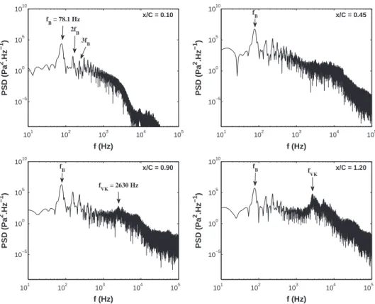
All the spectra show the appearance of the buffet frequency, at fB¼ 78:1 Hz (St ¼ fC=U1¼ 0:075), and its harmonics. In

the experiment, this frequency was equal to 69 Hz (St ¼0.066). At the most upstream position (x=C ¼ 0:10), the spectrum does not display any predominant frequency beyond 4000 Hz. Farther downstream (x=C ¼ 0:45), the spectrum displays a more significant spectral amplitude and more rich turbulence content in the area beyond 4000 Hz. This occurs because of the influence of the separated region downstream of the SWBLI. At this position, the spectrum can be compared with the

experimental results (Jacquin et al., 2009, Fig. 10). In the range of frequencies available on the spectrum from the

experiment, both spectra are similar in terms of the buffet frequency and its harmonics, although the shape of the peaks are different, which is due to the number of buffet periods (order of 20) in the numerical study which is less than in the experimental study. At this farther downstream position, the main mode is amplified and secondary oscillations at a higher frequency appear. This phenomenon becomes more pronounced for positions near the trailing edge (x=C ¼ 0:90) and in the

near-wake (x=C ¼ 1:20; see Fig. 8). At x=C ¼ 0:90, the power spectral density distribution can be compared with other

URANS simulations (Brunet et al., 2003, Figs. 11 and 18). The comparison of the spectral peak amplitude and their frequency

are close between the present study and the above reference. A frequency peak appears at around 2600 Hz (St ¼2.5). This peak becomes more pronounced at x=C ¼ 1:20.

We can show that this frequency corresponds to the von Kármán vortex shedding.Fig. 11presents snapshots of the

vorticity field taken at four equidistant time intervals in respect of the period 1/2600 s. These fields clearly show the alternating von Kármán vortex shedding and the periodicity of the vortex pattern from t¼0.00962 s to t¼0.01 s. In order to quantify the frequency of this vortex shedding, a tracking of the vorticity values versus time has been carried out at the

locations 1 and 2 (seeFig. 11) during one buffet period. The vorticity signals and their spectra are presented inFig. 12, where

a bump is identified at 2600 Hz. This fact insures the identification of a von Kármán mode at the present frequency. The peak localized at 2600 Hz in the spectra of the pressure signals is characterised by a spreading of frequencies (spectral ‘bump’). This is mainly due to a strong interaction of the von Kármán mode with the trailing-edge unsteadiness

(appearance of grey fringes related to Kutta waves in the div(U) plots,Fig. 8) and to the turbulent motion. This spectral

region is studied in more details in the next section, by means of time–frequency analysis.

Moreover, the Kelvin–Helmholtz vortices shown inFig. 8(c) in the detached shear layer downstream of the shock foot

can be identified by tracking them during the time-interval of 0.24μs. Their convection velocity has been assessed of order

101 102 103 104 105 10−5 100 105 1010 f (Hz) PSD (Pa 2.Hz −1 ) x/C = 0.10 f B = 78.1 Hz 2f B 3f B 101 102 103 104 105 10−5 100 105 1010 f (Hz) PSD (Pa 2 .Hz −1 ) x/C = 0.45 f B 101 102 103 104 105 10−5 100 105 1010 f (Hz) PSD (Pa 2.Hz −1 ) x/C = 0.90 f B f VK = 2630 Hz 101 102 103 104 105 10−5 100 105 1010 f (Hz) PSD (Pa 2 .Hz −1 ) x/C = 1.20 f VK f B

Fig. 10.PSD of the wall-pressure fluctuations at locations x=C ¼ 0:10, 0.45 and 0.90 on the airfoil surface and at point x=C ¼ 1:20, y=C ¼ 0:03 in the wake.

(14)

202 m * s! 1_{, as well as their wavelength,}_λ_{, of order 1:9 ' 10}! 2_{m. From these parameters, their shedding frequency has}

been assessed of order 104Hz (St ¼9.5) from the relation Uconv¼λ* f . This is higher than the von Kármán frequency. By

considering the energy spectrum at x=C ¼ 1:20 and y=C ¼ 0:03 with suitable window size and zero padding in order to better

visualize the region of frequencies around 104 _{Hz (}_{Fig. 13}_{), a predominant frequency peak at 10}4_{Hz can be identified, which}

corresponds to the Kelvin–Helmholtz shedding frequency.

As previously mentioned, the buffet frequency is found 78.1 Hz in the current study, while the vortex shedding frequency is about 2600 Hz when this phenomenon is well established. The ratio of these two frequencies is 33.29. The closest buffet harmonic regarding the von Kármán peak is 78.1 ' 33¼2577 Hz. This frequency slightly varies inside each buffet cycle, and from a cycle to another, which produces the bump observed in the spectra around 2600 Hz. This increases the uncertainty of

this frequency value. As shown in the spectrum ofFig. 14, the higher buffet harmonics “merge” with the von Kármán bump

onset and a synchronization may occur with von Kármán subharmonics. This interaction is difficult to analyse because the amplitudes of these higher harmonics and subharmonics are somehow “hidden” in the continuous part of the spectrum between the two events, the buffet and the von Kármán frequency peaks.

It is recalled that the present study aims at analysing the trailing-edge instabilities in association with the buffet mode.

The fluctuations related to the von Kármán instability appear less explicitly in the spectra inJacquin et al. (2009),Deck

(2005), as well as inThiery and Coustols (2005)andBrunet et al. (2003), because the main objective of these studies focused on the buffet phenomenon. Indeed, these studies measure the pressure fluctuations on the airfoil wall, with the most downstream position of the measurements located at x=C ¼ 0:90, where the level of the von Kármán fluctuations is still very small and the experimental spectrum cut-off is lower than the expected von Kármán frequency, captured by the present numerical study, which displays existence of a spectral bump region around a predominant frequency of order 2600 Hz

Fig. 11.Four instantaneous vorticity fields covering one period of trailing-edge vortex shedding and showing probing locations of the vorticity values used in next figure. 0 0.002 0.004 0.006 0.008 0.01 0.012 −1 −0.5 0 0.5 1 x 104 Time (s) Vorticity (s −1 ) Loc 1 Loc 2 103 104 10−5 100 105 Frequency (Hz) PSD (s −2 .Hz −1 ) Loc 1 Loc 2 f VK

Fig. 12.Vorticity signals in the wake (left) and their power spectral density (right).

(15)

In Fig. 20 of the experimental study by Jacquin et al. (2009), which displays four instants of the phase-averaged longitudinal velocity field, there is no proof of vortex shedding as identified in our study. This can be explained because a section of the wake is not visible due to the experimental setup, and also because the phase averaging, based on the buffet cycle, may have erased the marks of the vortex shedding, which has a frequency more than 30 times higher than the buffet

one, and a phase which is not synchronized with the buffet.Figs. 15and16of the present study show the instantaneous and

the phase-averaged longitudinal velocity fields respectively, at four phases of the buffet cycle, similarly to the experimental

results ofJacquin et al. (2009). These figures show the periodic motion of the accelerated region due to the buffet, as well as

the boundary-layer detachment. In fact, the von Kármán vortices are visible in the instantaneous fields using a similar color

scale as in the experimental results, but they are attenuated after phase-averaging over two buffet periods only (Fig. 16).

Regarding Fig. 12 ofDeck (2005)that displays the divergence of the velocity field, the color scale can be adapted in order to

highlight the vortex shedding structures, as the divergence of velocity is much smaller within the vortices than in the area of the shock wave and Kutta waves. However, an alternating pattern can be distinguished in this figure too. If the above mentioned studies had been interested in the near-wake region and under the condition that the experimental and numerical grids be sufficiently fine in the wake, they would have been able to capture the von Kármán instability too. However, this was not an objective of the mentioned studies. An evidence of the existence of the von Kármán mode in these experiments can be seen in the appearance of secondary fluctuations observed in the experimental measurements of the

time evolution of the pressure at x=C ¼ 0:45 (Jacquin et al., 2009, Fig. 8). If the spectrum of Fig. 10 inJacquin et al. (2009)

would display a frequency range beyond 103_{Hz, the von Kármán mode would also appear. This mode is characterised by a}

spectral bump, showing that it is subjected to the influence of other, more chaotic events in the time-space evolution.

Moreover, small vortices in the trailing-edge region have been measured byBrunet et al. (2003), in URANS simulations of

the OAT15A test case, but at a higher angle of attack (α¼51). Their signature seems to appear as a spectral bump in Fig. 11 of

this reference. These vortices can also be observed in the Schlieren visualization inFig. 7. Von Kármán vortices were also

reported in several experiments on subsonic compressible flows around airfoils (Alshabu and Olivier, 2008;Fung, 2002) as

well as in the direct simulation of transonic buffet at lower Reynolds numbers byBouhadji and Braza (2003b)andBourdet

et al. (2003). 103 104 100 102 104 f (Hz) PSD (Pa 2 .Hz −1 ) x/C = 1.20 f KH f VK

Fig. 13.PSD of pressure fluctuations at x=C ¼ 1:20, y=C ¼ 0:03. Detailed view of the range 103

!3 ' 104Hz. 101 102 103 104 105 10−5 100 105 1010 f (Hz) PSD (Pa 2 .Hz − 1 ) x/C = 1.20 f f B VK

Fig. 14.PSD of pressure fluctuations at x=C ¼ 1:20, y=C ¼ 0:03.

(16)

3.2.2. Time–frequency analysis

The pressure signal in the wake at x=C ¼ 1:20, a position where the amplitude of the secondary instabilities is maximum,

corresponding to the bursts formed in the pressure evolution and to the spectral “bumps” (Figs. 9and10respectively), are

governed by the von Kármán mode and instabilities mainly coming from the trailing edge and the shear layers. This signal is filtered by a high-pass filter with a cutoff frequency of 1577 Hz, by means of Fast Fourier Transform (FFT). The filtered

pressure signal, shown inFigs. 17and18, designated as Pf(f standing for filtered), is reconstructed by the inverse FFT. The

physical phenomena whose frequency is higher than 1577 Hz are conserved. The remaining signal shows now more clearly the buffet effect on the higher-frequency phenomena within each buffet cycle (burst). Each burst contains an order of 15 counter-rotating vortex-shedding pairs, as well as time intervals where the vortex shedding is considerably attenuated. The instability evolution within the burst is studied by means of time–frequency analysis, carried out by a continuous wavelet

Fig. 15.Instantaneous longitudinal velocity at 4 phases of a buffet cycle: (a) shock upstream; (b) shock moving downstream; (c) most upstream position of the shock; (d) shock travelling upstream.

Fig. 16.Phase-averaged longitudinal velocity at 4 phases of a buffet cycle: (a) shock upstream; (b) shock moving downstream; (c) most upstream position of the shock; (d) shock travelling upstream.

(17)

analyse two buffet periods: ψð Þ ¼t 1ffiffiffi 4 p πe 2iπf0t_e! t2=2_; _ð4Þ

where f0is the central frequency of the wavelet.

The wavelet transform coefficients are defined as

C a; bð Þ ¼ 1ffiffiffi a p Z 1 ! 1 x tð Þψn t !b a + , dt ð5Þ

where a and b are the scaling (in frequency) and the location (in time) parameters of the wavelet respectively, x(t) the signal

andψn

is the complex conjugate of the wavelet. The absolute value of these wavelet transform coefficients, jC Cn

j, is plotted inFig. 17. The scalogram allows analysing in more details the evolution of the vortex shedding frequency versus time inside

each buffet cycle. When the shock starts moving upstream (Fig. 8(b)), the vortices are shed at a frequency of 4000 Hz with

low amplitudes (see beginning of the burstFig. 17). Afterwards, this frequency diminishes to reach 2600 Hz, which is the

von Kármán frequency observed in the spectra. The vortex shedding is then well established within the burst and is

maintained until the shock reaches its most upstream position (see evolution of the shock motion,Fig. 8(c)–(f)). Next, the

generated vortices become smaller (Fig. 8(g)) and the shedding frequency increases to reach again the initial value of

4000 Hz, before this phenomenon be significantly attenuated and vanish while the shock moves downstream and the

boundary layer becomes attached (Fig. 8(h)–(a)). This frequency modulation, associated with the location and size of

the alternating vortices versus time, is linked to the spectral bump appearance around the von Kármán mode (Fig. 10). The

repetitiveness of this modulation is clearly observed in the scalogram. The first harmonic is also present with the same

modulation.Fig. 18presents the frequency variation of the pressure coefficient versus time during one buffet period, by

using the Yule–Walker autoregressive (AR) model. This kind of model conceptually ensures a high accuracy in the estimation

of the frequency values versus time (Braza et al., 2001). The Yule–Walker equations, obtained by fitting the autoregressive

−15000 −10000 −5000 0 5000 P (Pa)f Time (s) Frequency (Hz) 0 0.005 0.01 0.015 0.02 0.025 1000 2000 3000 4000 5000 6000 7000 8000 9000 10000 |CC*| 0 0.1 0.2 0.3 0.4 0.5 0.6 0.7 0.8

Fig. 17.Normalized absolute value of complex continuous wavelet transform coefficients.

−15000 −−100005000 0 5000 0 0.002 0.004 0.006 0.008 0.01 0.012 0.014 2000 3000 4000 5000 6000 7000 8000 Time (s) P (Pa)f Frequency (Hz)

Fig. 18.Time–frequency analysis of the filtered pressure signal at x=C ¼ 1:20, y=C ¼ 0:03, using autoregressive modelling.

(18)

linear prediction filter model to the signal, by minimizing the forward prediction error in the least squares sense, are solved

by the Levinson–Durbin recursion (Durbin, 1960). This method is applied with an AR order of 210 on a signal including a one

burst cycle. 14 952 samples are used and the signal is segmented in windows of 1153 points. The fundamental frequency of

each segment is obtained by calculating the PSD of the modelled signal, using zero-padding giving 221_{samples. The result of}

this method shows the same frequency modulation during the vortex shedding occurrence, as in case of the continuous wavelet transform.

In the next section, a POD analysis is presented which includes additional aspects of the interaction among the buffet, the von Kármán and the smaller-scale higher-frequency vortices, especially those of the shear layers.

3.2.3. Proper orthogonal decomposition

Based on the time-space solution from the previously mentioned simulations, a proper orthogonal decomposition (POD) has been carried out on the ensemble-averaged flow-fields, based on the separable POD method in respect of space and time (Sirovich, 1990;Aubry et al., 1991), as presented in the following relations. The POD modes are evaluated from a series of successive snapshots, which include in the present case 10 buffet periods. 646 snapshots, recorded by using a sampling rate

of 10!5_{s, are used per buffet period. As the first POD mode corresponds to the time-averaged solution contained in the data,}

the POD modes from order 2 correspond to the fluctuating part of the velocity fields:

Uðx; tÞ ¼ UðxÞþuðx; tÞ ¼ UðxÞþX

NPOD

n ¼ 2

anðtÞϕnðxÞ; ð6Þ

where U and u denote the mean and fluctuating parts of the velocity, respectively. The fluctuation mainly includes the effects of the buffet, von Kármán and shear-layer instabilities. This fluctuation includes the following contributions:

uðx; tÞ ¼ ~uðx; tÞþ "uðx; tÞþ ^uðx; tÞ; ð7Þ

where ~uis the phase-averaging, "uis the downscale contribution of the fluctuation, and ^u is the upscale one. Following a

simple algebraic development for the decomposed phase-averaged Navier–Stokes equations, it can be shown that the new turbulent stresses contain a downscale part: 〈 "uiu"j〉, and a cross term: ^Rij¼ 〈 "uju^i〉þ〈 ^uju"i〉þ〈 ^uju^i〉. As will be discussed in the

next section, ^Rijwill be modelled by a stochastic forcing. At this stage, a major contribution is due to the downscale term.

The normalized shape-functionsϕnare spatially orthogonal, while the temporal coefficients anare uncorrelated in time:

ϕ_i*ϕ_j

D E

¼δij and aiaj¼δijλi: ð8Þ

The brackets and overbar indicate spatial integration and temporal averaging, respectively.λiis the eigenvalue of mode i.

δijis the Kronecker delta. The POD modesϕnare obtained as the eigen-modes of the two-point correlation matrix:

Cϕn¼λnϕn with Cij¼ uðxi; tÞ * uðxj; tÞ: ð9Þ

The eigenvalueλnrepresents the contribution of the corresponding POD mode to the total fluctuating energy:

uðxi; tÞ * uðxj; tÞ 0 1 ¼ X NPOD n ¼ 1 λn: ð10Þ

Fig. 19shows the energy of the POD modes as a function of the mode order. There is an energy decrease towards the

0 20 40 60 80 100 10−6 10−4 10−2 100 Modes Energy (%) 100 101 102 10−6 10−4 10−2 100 Modes Energy (%)

Fig. 19.Energy distribution of the POD modes (semi-log and log–log diagrams).

(19)

becomes more pronounced, as the mode order increases. A similar behaviour was reported in experimental studies by

Perrin et al. (2006).

The POD analysis allows extracting the most energetic modes (Fig. 20) which can reconstruct the main features of the

interaction between the buffet and the downstream region as shown in the following. The modes 2 and 3 of the streamwise

velocity U illustrate the buffet phenomenon and the boundary-layer intermittent detachment (Fig. 20).

Modes 4 and 5 clearly illustrate the von Kármán motion. A complex interaction among the buffet region (shock), the shear layer past the SWBLI and the von Kármán mode past the trailing edge is shown by means of the higher order modes. This interaction leads to creation of a more pronounced chaotic process (modes 6 and 7), because the frequencies of the mentioned instabilities are incommensurate. Furthermore, the von Kármán mode iso-contour levels affect also the shock-motion region (modes 4–9).

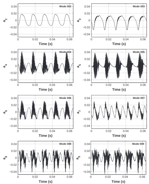
The temporal POD coefficients are shown inFig. 21. They are in accordance with the spatial mode behaviour. As the order

of the modes increases, a filling-up of the temporal coefficient signal by higher frequencies is noticed, showing the increasing complexity of the dynamic system, due to turbulence.

The energy spectra of the temporal POD coefficients for modes 2–9 are presented inFig. 22. The first spectrum indicates

the buffet frequency as a predominant one and confirms the fact that mode 2 is associated with this instability. The POD modes higher than 3 start progressively to be affected by the von Kármán instability, as shown also in the spatial

distribution of these modes,Fig. 20. The amplitude of the von Kármán instability (Fig. 22) increases for modes 4 and 5, to

reach a practically invariant level in the higher mode spectra. Simultaneously with this variation, the buffet instability amplitude decreases on the spectra and its harmonics slightly increase but the global level of the buffet instability amplitude remains lower than in case of the third POD mode. Therefore, in the mode ranges 4 and 5, the spectral amplitudes of the von Kármán and of the buffet become comparable.

Fig. 20.First POD modes associated with the streamwise velocity.

(20)

From the dynamic system theory point of view, a non-linear interaction between two incommensurate instability modes that are rather close in terms of frequency produces linear combinations of these two modes in the energy spectrum (Newhouse et al., 1978;Guzmán and Amon, 1994). In the POD spectrum of mode 2 (Fig. 22), the interaction between the higher buffet harmonics and the von Kármán subharmonics is more visible, because these two sets are neighbours. We can

detect for example a predominant frequency bump, fi1, which can be expressed as fVK=2 !5fB. Moreover, a second

interaction can be extracted, fi2¼ fVK=2 !8fB. These interactions, as in the aforementioned papers, do not considerably

change the frequency values of the instability modes (buffet and von Kármán). They rather change the amplitudes of these

modes, which become comparable between the buffet mode and the von Kármán, as shown in Fig. 22(spectra of POD

modes 4 and 5, as well as spectra of POD modes 6 and 7). This illustrates a way the buffet mode is affected by the shedding mode and vice-versa.

The spectra of modes 12 and 13 are presented inFig. 23. They show a broadening of the von Kármán area associated with

the interaction between smaller-scale higher-frequency vortices (as for example the K–H around 104_{Hz) and more chaotic}

0 0.02 0.04 0.06 −0.04 −0.02 0 0.02 0.04 Time (s) a 2 Mode 002 0 0.02 0.04 0.06 −0.04 −0.02 0 0.02 0.04 Time (s) a 3 Mode 003 0 0.02 0.04 0.06 −0.04 −0.02 0 0.02 0.04 Time (s) a 4 Mode 004 0 0.02 0.04 0.06 −0.04 −0.02 0 0.02 0.04 Time (s) a 5 Mode 005 0 0.02 0.04 0.06 −0.04 −0.02 0 0.02 0.04 Time (s) a 6 Mode 006 0 0.02 0.04 0.06 −0.04 −0.02 0 0.02 0.04 Time (s) a 7 Mode 007 0 0.02 0.04 0.06 −0.04 −0.02 0 0.02 0.04 Time (s) a 8 Mode 008 0 0.02 0.04 0.06 −0.04 −0.02 0 0.02 0.04 Time (s) a 9 Mode 009

Fig. 21.Temporal coefficients anof the first POD modes. D. Szubert et al. / Journal of Fluids and Structures 55 (2015) 276–302

(21)

Based on the present discussion, the POD analysis illustrates in a complementary way the interaction between the buffet and the von Kármán modes as well as with the higher frequency structures, by means of the mode shape and the temporal coefficients amplitude modulations, as well as by the appearance of new frequency peaks in the spectra combining these instabilities. 101 102 103 104 10−15 10−10 10−5 f (Hz) PSD (Pa 2 .Hz −1 ) Mode 002 f B 2f_B_3f B 5f B f i2 fi1 4f_B 101 102 103 104 10−15 10−10 10−5 f (Hz) PSD (Pa 2.Hz −1 ) Mode 003 2702 Hz 101 102 103 104 10−15 10−10 10−5 f (Hz) PSD (Pa 2.Hz −1 ) Mode 004 101 102 103 104 10−15 10−10 10−5 f (Hz) PSD (Pa 2.Hz −1 ) Mode 005 101 102 103 104 10−15 10−10 10−5 f (Hz) PSD (Pa 2.Hz −1 ) Mode 006 101 102 103 104 10−15 10−10 10−5 f (Hz) PSD (Pa 2.Hz −1 ) Mode 007 101 102 103 104 10−15 10−10 10−5 f (Hz) PSD (Pa 2.Hz −1 ) Mode 008 101 102 103 104 10−15 10−10 10−5 f (Hz) PSD (Pa 2.Hz −1 ) Mode 009

Fig. 22.PSD of POD mode temporal coefficients.

(22)

Furthermore, the POD analysis illustrates the signature of the Kelvin–Helmholtz vortices (Figs. 24–26). In the 12th and 13th POD mode fields, the development of the lower shear-layer structure past the trailing edge can be observed. In the 24th

and 26th mode fields, the impact of the upper shear-layer vortices can be seen. The higher POD modes (Fig. 26) influence all

the high shearing rate regions, including also the shock area. Therefore, these figures show the filling of the shear layers by smaller-scale structures and illustrate their interactions with the shock-motion area. Indeed, the iso-contour levels of these

smaller structures fill up the shock-motion region (Figs. 25and26).

4. Stochastic forcing by means of POD

The shear-layer interfaces between the turbulent and non-turbulent regions are now considered in association with those POD modes which particularly affect these areas as previously discussed. In order to maintain these interfaces thin and to limit the turbulent diffusion effect due to the direct cascade modelling assumptions, a small amount of kinetic energy

is introduced as a “forcing” in the transport equations of the k andεvariables, acting as a “blocking effect” of the vorticity in

the shear layer as in the schematic representation ofFig. 1, according toWesterweel et al. (2009). This small kinetic energy

can be constructed from the “residual” high-order POD modes previously presented, by reconstructing fluctuating velocity components derived from the use of the last POD modes of very low energy. Therefore, an inhomogeneous stochastic forcing

can be built and used as a source term in the transport equations regarding k (Eq.(11)) andε(Eq.(12)). This term contains a

101 102 103 104 10−15 10−10 10−5 f (Hz) PSD (Pa 2.Hz −1 ) Mode 012 101 102 103 104 10−15 10−10 10−5 f (Hz) PSD (Pa 2 .Hz −1 ) Mode 013

Fig. 23.PSD of temporal coefficient of POD modes 12 and 13.

Fig. 24.POD modes 12 and 13 associated with the streamwise velocity.

Fig. 25.Intermediate-range POD modes associated with the streamwise velocity.

(23)

turbulence intensity and ~r is taken from a random number generator varying in the interval ½0; 1.. This form is similar, from a

dimensional point of view only, to the homogeneous ambient terms introduced bySpalart and Rumsey (2007)in order to

sustains the turbulent kinetic energy level specified in the upstream conditions, which usually decays towards the body due to the dissipation rate:

Dk Dt ¼P !εþ ∂ ∂xi νþ νt σk + _{, ∂}_k ∂xi 2 3 þSPOD ð11Þ

Fig. 26. Higher-range POD modes associated with the streamwise velocity.

101 102 103 104 10−15 10−10 10−5 f (Hz) PSD (Pa 2.Hz −1 ) Mode 060 101 102 103 104 10−15 10−10 10−5 f (Hz) PSD (Pa 2 .Hz −1 ) Mode 061 101 102 103 104 10−15 10−10 10−5 f (Hz) PSD (Pa 2.Hz −1 ) Mode 078 101 102 103 104 10−15 10−10 10−5 f (Hz) PSD (Pa 2 .Hz −1 ) Mode 079

Fig. 27.PSD of temporal coefficient of higher POD modes.

(24)

Dε Dt ¼ ε kðCε1P !Cε2εÞþ ∂ ∂xi νþ νt σε + _{, ∂} ε ∂xi 2 3 þCε2S 2 POD kamb ð12Þ with

SPOD¼ ~rCμðk2ambþk2PODÞ=νt1; ð13Þ

andνt¼ Cμk2=εis the turbulent viscosity.νt1is the freestream turbulent viscosity.

In the present study, this source term is derived from the local-scale, higher-order POD modes. InFig. 26, the

higher-order POD shape modes,ϕnðxÞ, are maximum in the regions where the shearing rate is high (shear-layer and shock regions).

In the present study, an order of the last 40 modes (from 60th to 99th) have this property, as shown in the previous section. This approach may be adapted for other cases. These POD modes are associated with the temporal coefficients by using the

relation(6)in order to produce a reconstruction of the velocity components and to calculate a low-energy velocity scale,

ffiffiffiffiffiffiffiffiffiffiffiffiffiffiffi

u2_þv2

p

. This reconstruction used the whole snapshot sequence of 10 buffet periods as for the previous POD analysis. In this

way, an averaged turbulent kinetic energy scale, kPOD, is calculated as: kPOD¼ 0:5 ' ðu2þv2Þ. As a first approximation, a

time-averaged kinetic energy is evaluated. These equations are time-dependent and yield to a solution with temporal variation of

the shear-layer as in Fig. 8. These source terms lead to a forcing of the turbulent stresses by means of the turbulence

behaviour law and the turbulent viscosity. The new stresses act as an energy transfer from the stochastic small-scale modes to the higher ones.

As mentioned above, this stochastic forcing is simultaneously localised in the shear layer, in the wake and in the shock wave areas, thanks to the properties of the higher-order POD modes presented in the previous section, without

contaminating the neighboring regions, which remain irrotational, as shown in the spatial distribution of kPOD,Fig. 28.

The time-dependent evolution of these regions is taken into account. As will be discussed, the solution is now improved in respect of the shear-layer thinning.

Fig. 29shows the divergence of the velocity vector at eight representative instants within the buffet period, according to

the simulation including the stochastic forcing detailed above. A qualitative comparison withFig. 8shows a reduced

shock-motion amplitude, which is in good agreement with the experiment. Furthermore, the shear layer and separated regions, which remain time-dependent, are thinner than in the previous case without stochastic forcing. These facts are quantified in

Figs. 30,32and33.

Fig. 30shows a comparison of the mean surface pressure distribution between k !ε-OES and its variants with the

experimental results. “amb” stands for the homogeneous ambient terms described inSpalart and Rumsey (2007), and “IOES”

(I standing for “improved”) refers to the modelling by stochastic forcing involving the kPOD field as discussed at the

beginning of this section. The k!ε-OES without ambient terms provides a larger shock amplitude than in the experiment.

The k!ε-OES with the homogeneous ambient terms provides an improvement in the shock-amplitude motion compared to

the basic k!ε-OES simulation. In the IOES case, the pressure coefficient shows an even improved shock-motion amplitude

where the shock-motion amplitude is large, as well as a better estimation of the pressure distribution in the region from the most downstream position of the shock to the trailing edge. This can be explained by the fact that the ambient terms and the stochastic forcing “add” a slight level of eddy viscosity in the OES modelling which is designed to reduce the eddy viscosity and to allow the instability development. Therefore, the instability development becomes slightly moderate by

Fig. 28.Averaged turbulent kinetic enery field, kPOD, issued from fluctuating velocity reconstruction for higher-order modes 60–99. D. Szubert et al. / Journal of Fluids and Structures 55 (2015) 276–302

(25)

The TNT (Turbulent/Non-Turbulent) interface is localized where the vorticity gradient across the interface is maximum.

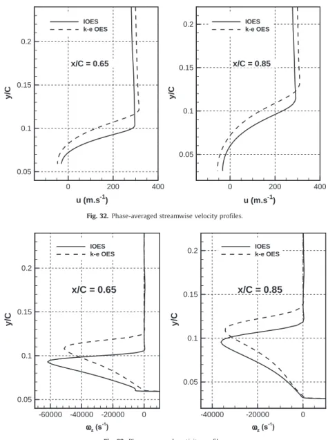
The phase-averaged velocity and vorticity profiles derived from the k!ε-OES model, as well as from the IOES at the same

phase, are compared inFigs. 32and33at two positions: x=C ¼ 0:65 and x=C ¼ 0:85.

Fig. 31shows the two locations where the phase-averaged velocity and vorticity profiles have been extracted at the same buffet phase to compare the stochastic forcing effects to the basic simulation.

Fig. 32shows the comparison of these velocity profiles according to both approaches. It can be seen that the simulation

with the forcing (IOES) leads to a significant thinning of the shear layer. This can also be observed inFig. 33, where the two

Fig. 29.Instantaneous fields of velocity divergence – application of the inhomogeneous stochastic forcing (Tbis the buffet period). D. Szubert et al. / Journal of Fluids and Structures 55 (2015) 276–302 297

(26)

approaches are compared by means of the vorticity. The TNT interface, identified by a vorticity close to 0, is lowered by using the stochastic forcing. Its thickness is reduced by 30% at x=C ¼ 0:65, and by 19% at x=C ¼ 0:85, which has as a consequence the reduction of the drag, due to the reduction of the viscous region downstream of the shock. The present inhomogeneous

forcing reproduces the blocking and thinning effect, similarly to the DNS results ofIshihara et al. (2015)regarding

boundary-layer interface.

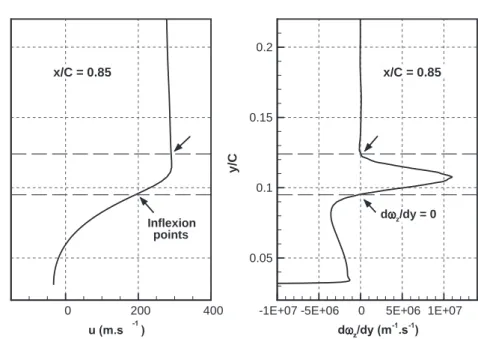
Fig. 34left shows the velocity profile at the location x=C ¼ 0:85, as well as the vorticity gradient profile at the same

position (Fig. 34right). Two inflexion points of the velocity profile are identified, corresponding to the change in sign of the

vorticity gradient (dω=dy ¼ 0). The existence of the inflexion points is associated indeed with the shear-layer instability

development, illustrated inFig. 29as well as with the small series of Kelvin–Helmholtz vortices captured by the present

simulation.

Following these results concerning the improved velocity profiles, a theoretical instability study can be carried out on the basis of the present velocity profiles in a future study, in order to accurately determine the critical shear rate beyond which the mentioned instabilities are amplified.

5. Conclusion

The present numerical study analyses in detail the flow physics of the transonic shock-wave, shear-layer and wake interaction around a supercritical airfoil at high Reynolds number (3 million), incidence of 3.51 and at a Mach number of 0.73. This set of physical parameters corresponds to the onset of the buffet instability, a challenge for the prediction of this instability appearance near the critical parameters by numerical simulation including turbulence modelling in the high-Reynolds number range. This study describes a new approach highlighting the dynamics of the transonic buffet in interaction with the near-wake von Kármán instability as well as with smaller-scale vortex structures in the separated shear layers, related to the Kelvin–Helmholtz instability.

This analysis is carried out by the Organized Eddy Simulation (OES) method, which resolves the organized coherent structures and models the random turbulence by adapted statistical modelling. This method has been improved in the

x/c Cp 0 0.2 0.4 0.6 0.8 1 -1.5 -1.0 -0.5 0.0 0.5 1.0 EXP k-e OES k-e OES + amb IOES

Fig. 30.Comparison of the mean surface pressure coefficient distribution between experiment, basic k!ε-OES modelling, k!ε-OES using the ambient terms ofSpalart and Rumsey (2007): k!ε-OES þ amb, stochastic forcing formulated in this study: IOES.

Fig. 31.Location of the phase-averaged velocity and vorticity profiles.

(27)

By means of this modelling approach, the study contributes to complete experimental physical analysis of the transonic buffet, which was mainly interested in the shock motion and pressure-velocity distributions around the body and less in the interaction with the wake instabilities in the related literature. This study provides new results regarding the buffet interaction with the von Kármán mode and the smaller-scale vortex structures. The Proper Orthogonal Decomposition analysis has shown that this interaction creates an amplitude modulation of the buffet mode due to the von Kármán mode and vice-versa. The wavelet and autoregressive model analysis quantified a frequency modulation of the von Kármán instability due to the buffet. The predominant frequencies of these modes have been evaluated by spectral analysis and the interaction among them has been illustrated by the appearance of new frequencies in the energy spectrum, being combinations of the principal instability modes. Whereas the buffet mode is a well distinguished frequency peak in the spectrum, the von Kármán mode is characterized by a spectral ‘bump’ appearance around a frequency 33.3 times higher than the buffet frequency. The spectral analysis has shown the modification of the von Kármán mode ‘bump’ shape due to higher-order buffet harmonics and the amplification of the K–H instability peak of higher frequency.

Concerning these interactions, the POD analysis distinguished the shape modes involved in the formation of highly energetic coherent vortices and of the buffet dynamics from those of weaker energy involved in smaller-scale vortex structures appearing in the shear layers and influencing also the shock-motion area.

u (m.s-1) y /C 0 200 400 0.05 0.1 0.15 0.2 IOES k-e OES x/C = 0.65 y /C 0 200 400 0.05 0.1 0.15 0.2 IOES k-e OES x/C = 0.85 u (m.s-1)

Fig. 32.Phase-averaged streamwise velocity profiles.

y /C -60000 -40000 -20000 0 0.05 0.1 0.15 0.2 IOES k-e OES x/C = 0.65 y /C -40000 -20000 0 0.05 0.1 0.15

0.2 IOES_{k-e OES}

x/C = 0.85

Fig. 33.Phase-averaged vorticity profiles.