This is an author-deposited version published in:
http://oatao.univ-toulouse.fr/
Eprints ID: 14714
To cite this version:
Nouasse, Houda and Chiron, Pascale and Archimède, Bernard Supervisory
control of river flood: network modeling with varying time delay. (2014)
In: 10th International Conference on MOdeling, Optimization and
SIMlation - MOSIM14, 5 November 2014 - 7 November 2014 (Nancy,
France).
O
pen
A
rchive
T
oulouse
A
rchive
O
uverte (
OATAO
)
OATAO is an open access repository that collects the work of Toulouse researchers and
makes it freely available over the web where possible.
Any correspondence concerning this service should be sent to the repository
administrator:
[email protected]
SUPERVISORY CONTROL OF RIVER FLOOD: NETWORK
MODELING WITH VARYING TIME DELAY
H. Nouasse, P. Chiron, B. Archim`ede
University of Toulouse, INPT, ENIT, LGP 47 av. d’Azereix BP 1629
65016 TARBES cedex - France
[email protected], [email protected], [email protected]
ABSTRACT: Food phenomena become an usual phenomenon occurring in the world and causing serious
human and material damage. One way to protect urban zones from river floods is to equipped river with flood control area used as reservoirs in order to reduce the velocity of water and to attenuate the flood wave. The work presented in this paper concerns the supervisory control of such an equipped river. The supervisory scheme consists in four blocks connected to the river process: a Supervisory Control and Data Acquisition block, a Dynamic Parameterization block, a Diagnosis-Decision-Correction block and a Management Objectives and Constraints Generation block. The proposed method is based on a dynamic method combining a reduced transportation network and a temporized matrix from which the water volumes to be stored or released in time are calculated. It makes possible the water storage and release adapted to each river flood scenario, and preservation of agriculture in these floodplains. It takes into account the variation of the time delay with the flow without any modification in the structure of the network.
KEYWORDS: Water systems management, Supervisory control, Transportation networks, Time
de-lay, Flood control.
1 INTRODUCTION
Flood is an usual phenomenon all over the world. Ex-treme rainfall events become more frequent and the induced damages more severe. Recently, at the end of April 2014, rainstorm caused floods in the North of Florida, as well as in the east of the United States, rains reached up to 550 millimeters of water. Roads were cut, a street collapsed in Baltimore, flights were delayed, hundred of people have been evacu-ated, power failure affected more than 28000 homes. This disaster caused the loss of 35 lives (source AFP). Flooding due to excessive rains can cause significant human and material damages around the world. One way to prevent these flood problems is to equipped river with flood control area used as reser-voirs. The reservoirs are emptying with water in or-der to reduce the water velocity in the river and to
attenuate the flood wave. Various research works
have been proposed in order to reduce flood peaks and volumes involving linear programming (Needham et al., 2000), folded dynamic programming (Nagesh Kumar et al., 2009), hybrid analytic/rule-based ap-proach (Karbowski et al., 2005) for example. Most of these methods do not allow controlling the dura-tion of water storage in the reservoir, the storage and
release dates ... In order to improve the managers’ decisions during these abrupt climatic phenomena, optimization techniques were proposed such as lin-ear programming (Karamouz et al., 2003), fuzzy opti-mization (Fu, 2008; Cheng and Chau, 2001), stochas-tic optimization (Ratnayake and Harboe, 2007) and multi-objective optimization (Chuntian and Chau, 2002). Rivers are equipped with sensors and actu-ators and Supervisory Control and Data Acquisition systems (SCADA) are developed in order to improve their control. Such SCADA systems are used to col-lect data from sensors, communicate with operators through a Human Machine Interface, and send con-trol values to actuators in many kind of systems such as irrigation canals (Figueiredo et al., 2013; Puerto et al., 2013; Pfitscher et al., 2012), inland navigation networks (Duviella et al., 2013), or energy manage-ment (Mora et al., 2012) ; network vulnerabilities of such systems are studied in (Amin et al., 2013a,b). In order to manage the water volumes in case of flood in river area, a supervisory control scheme is pro-posed in this paper. The structure of the paper is as follows. Section 2 describes the proposed scheme which includes water storage and release in the reser-voirs and the variation of time delay with discharge. The effectiveness of the proposed supervisory scheme
!"#$%&&' ()&*+,$-)./' 0%+&1"%2%.,&' 312+.' 0+$-).%' 4.,%"5+$%'' (+,+' 6+&%' ()&*+,$-)./' 0%+&1"%2%.,& 312+.' 0+$-).%' 4.,%"5+$%'' (+,+' 6+&%' 78 9 ( 9 ' (:.+2)$' *+"+2%; ,%")<+=#.' 0+.+/%2%.,'#>?%$=@%&'+.A'$#.&,"+).,&'/%.%"+=#.' 9A+*,+=#.' 9A+*,+=#. ()+/.#&)&;(%$)&)#.;8#""%$=#.' S P =#.' B)@%"' C8BD' C8BE' C8B"' C8B.F' FD' FE' F"' F.F' τD' τ";D' τ.F;D'
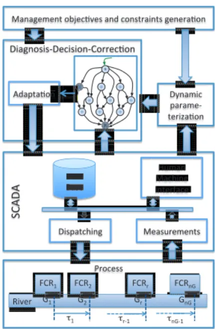
Figure 1 – Supervisory Control Scheme. is shown for different flood situations on a simulated river system in section 3. Finally, conclusion is given and some future works are suggested.
2 SUPERVISORY CONTROL SCHEME
2.1 General Scheme
In order to manage the water volumes in case of flood arising in river area, a supervisory control scheme de-picted in Figure 1 is proposed. The process is a river
system along which nG reservoirs are distributed.
Theses reservoirs, denoted F CRr(flood control
reser-voir) are floodplains provided with a controlled gate
Gr, r = 1, · · · , nG, and are used to absorb the flood.
The time delay, τr, from the gate Grto the following
gate Gr+1 depends on the flow discharge. The gate
opening should be computed in order to maintain the river discharge under a predefined flow value called the attenuation flow. Thus the control of discharges leads to limit the level of the river.
The SCADA system is connected to the river process. It transmits the sensors’ values to the Diagnostic-Decision-Correction and the Dynamic Parameteriza-tion blocks, and receives the gate opening values in order to send them to the process. The measurements considered herein are levels and discharges.
The Diagnostic-Decision-Correction block (DDC) permits the determination of the gate opening set-points. It is composed of a transportation network which diagnose the process state, depending on the flow in the river, decide if a correction must be carried out and execute it. The transportation network in-cludes time delays, moreover, if the time delays vary, it is not necessary to change the network structure (no need to add node or arc, only network
parame-ters are modified); as described in the next section (section 2.2). Setpoints values are adapted in order to be understood by the SCADA system.
The Dynamic Parameterization (DP) block provides the DDC block with all the necessary dynamic char-acteristics such as time delays.
The Management Objectives and Constraints Gen-eration block supplies the DDC and DP blocks with management constraints and rules such as the thresh-olds, the attenuation flow value, the priority param-eters.
2.2 Network With Time Delay
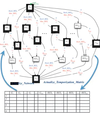
The river with FCR is modeled with a transporta-tion network including time delay. In previous work (Nouasse et al., 2012), we firstly proposed the use of a static transportation network, where time delay where neglected. Because of the importance of the flow delay in the river, the method was improved to include time delay (Nouasse et al., 2013a) and storage and release operations for reservoirs (Nouasse et al., 2013b). The method is composed of a transporta-tion network G and a Temporizatransporta-tion Matrix (T M ), as described in Figure 2. In these works, time delays were constant during the simulation; in the present paper, the method is proved to be efficient with delay varying during the simulation.
The objective of the method is to maintain the flow
under a predefined attenuation flow denoted Qlam.
The attenuation flow is a flow threshold under which the river flow should remain as, expected by the river system manager. Moreover, in order to protect agri-culture and to be able to control a new flood episode, when the reservoirs are not empty, and when the dis-charge level in the river is lower than the attenuation threshold, the stored water can be released. For this
purpose a threshold, Qdo, is defined as the discharge
level under which the water is released from the reser-voir. In the case of release, gates are opened in a way that the discharge level in the river remains under the
attenuation threshold Qlam.
In order to determine the optimal attenuation flow that satisfies the management objectives and the flood occurring case, we formulated the problem as a Min-Cost-Max-Flow problem. The cost function to minimize is subject to the constraints of flow con-servation and minimal and maximal capacities in the network. The network G enables water storage and release from reservoirs. In order to include variable transfer time in the network without oversizing it,
the values of delayed flow are stored in the n × 2nG
T M matrix. Each column represents the evolution of a gate or a FCR, and each line represents an in-stant of the evolution of the state of the system,
Actualize_Network Actualize_Temporization_Matrix
G1 G2 … Gr … GnG RES1 RES2 … RESr … RESnG 1 2 … k … n rk rk rk rk rk rk rk rk S 0 G 1 RES 1 RES 2 P 0 G 2 G nG RESnG Q ( k ) RD1 RD nG RD2 Stock_RES1 Max_RES1 1 0 Qpeak 1 0 λ1 1 0 Stock_RES1 1000 0 v1 1 0 Qpeak 100 Stock_RES1 Max_RES1 1 Stock_RES2 Max_RES2 1 0 α2 1 0 λ2 1 0 Stock_RES2 1000 0 v2 1 Stock_RES2 Max_RES2 1 0 Qpeak 100 Stock_RESnG Max_RESnG 1 0 Qpeak 100 0 vnG 1 0 Stock_RESnG 1000 0 λnG 1 0 αnG 1 Stock_RESnG Max_RESnG 1 RES r Gr RD r Stock_RESr Max_RESr 1 0 αr 1 0 λr 1 0 Stock_RESr 1000 Stock_RESr Max_RESr 1 0 Qpeak 100 0 vr 1
…
…
Figure 2 – Network for Diagnosis-Decision-Correction Block.
at each kTc, k = 0, · · · , n, in the horizon Hf, with
Hf = n × Tc, n ∈ N+.
The network G = {N , A} where N is a set of 3nG+ 2
nodes defined as follows, with r = 1, · · · , nG:
• The node Grrepresents the gate Gr;
• The node RDris a release decision node;
• The node RESris a reservoir node;
• The node S0 is a source node corresponding to
the fictive entry point of the system;
• The node P0is a sink node corresponding to the
fictive exit point of the system.
The arcs belonging to the set A between the nodes of N are valued, each value is between a maximum ca-pacity and a minimum caca-pacity written respectively
in blue and red in Figure 2. The arc value at kTc is
computed using an optimization algorithm as detailed in the following. The arcs describe the following con-nections:
• The arc between the node S0 and the node
RDr, r = 1, . . . , nG, represents the water
vol-ume already stored in the reservoir linked to it.
Its maximum capacity is M ax RESr, the
maxi-mum storage capacity of the reservoir, which de-pends on the maximum value of the peak
flow-rate of the flood (Qpeak). Its minimum
capac-ity is Stock RESr, and it corresponds to the
amount of water already present in the reservoir.
• The arc between the node RDr and the node
Gr, r = 1, . . . , nG, represents the draw-off flow
leaving the reservoir. Its maximum capacity is
denoted λr.
• The arc between the node RDr and RESr, r =
1, . . . , nG, represents the water volume not
re-leased and remaining in the reservoir at the end of the concerned period. Its maximum
capac-ity is Stock RESr, the amount of water already
present in the reservoir.
• The arc between the node S0 and the node Gr,
r = 2, · · · , nG, takes into account the discharge
upstream from the gate Gr in the system. Its
maximum capacity is Qpeak.
• The arc between the node Gr and the node
RESr, connects the gate with its reservoir. It
represents the flow leaving the river through the
gate Gr towards the reservoir, i. e. the stored
water. Its maximum capacity is denoted νr.
• The arc between the node Gr and the node P0,
r = 1, · · · , nG−1, represents the flow transferred
from the gate Grto the next gate Gr+1. This
dis-charge is stored in the column of T M associated
to the gate Gr+1 at line k + kr, with kr= ⌊τTrc⌋.
Its maximum capacity is Qpeak.
• The arc between the node GnGand the node P0,
corresponds to the flow-rate downstream from the exit point of the system. Its maximum
ca-pacity is Qpeak.
• The arc between the node RESr and the node
P0, r = 1, · · · , nG, represents the total volume
of water remaining in the reservoir. It respects transportation network conservation flow rules.
Its maximum capacity is M ax RESr, its
mini-mum capacity is Stock RESr.
In Figure 2, the cost of each arc is written in black. In order to limit overflow downstream, the cost of the
GnGP0arc is set to a high value, here 100. Similarly,
the cost of the GrP0arcs (r = 1, . . . , nG− 1) are set
to a value lower or equal to the GnGP0arc cost, here
100. In order to release water only in the case where
there is no overflow risk, the costs of the RDrRESr
arcs (r = 1, . . . , nG) were set to a value higher than
the cost value of the GnGP0 arc, here 1000. Finally,
the three reservoirs are considered to have a similar role, thus, all other costs were set equal to 1.
The Flood-Attenuation algorithm, described in al-gorithm 1, permits to determine the gate opening setpoint values. The computation of the setpoints is based on the arc values. Firstly, the temporiza-tion matrix is initialized. Thereafter, at each k, the network and the temporization matrix are actualized (see algorithm 2 and algorithm 3), the optimal flow is
Algorithm 1: Flood Attenuation
input :
Gthe network
n = ⌊Hf
Tc⌋ + 1 the number of samples
nG the number of gates and FCR in the system
kr= ⌊Tτr
c⌋, r = 1, · · · , nG− 1
Qinput(k) the flow of flood at kTc, k = 1 · · · n
Qlam the attenuation flow
output:
Gthe network
T M the n × 2nG temporization matrix
ϕ∗ the optimal flow for each arc in G
begin
% Initialization phase one
fork = 1 to n do T M (k, 1) ← Qinput(0) forr = 2 to 2nG do T M (k, r) ← 0 end end
% Initialization phase two
forr = 1 to nG− 1 do
fork = 1 to kr− 1 do
T M (k, r + 1) ← min(Qinput(0), Qlam)
end end k ← 1
while (k ≤ n) do
Actualize Network(G, k, T M )
ϕ∗(k) ← Compute Optimal Flow(G, k)
Actualize Matrix(ϕ∗(k), k, T M )
k ← k + 1 end
end
computed. In order to compute the optimal flow, the Min cost Max flow problem resolution for this net-work is done, using a Linear Programming formula-tion (as described in (Nouasse et al., 2012)), according
to our management objectives. ϕ∗
xy(k) is the obtained
optimal flow from node x to node y in the network
G at kTc; thus, at kTc, we can derive the gate Gr
opening setpoint value which is equal to ϕ∗
GrRESr(k)
in the storage case and to ϕ∗
RDrGr(k) in the release
case. During the phase one of the initialization of
the Flood-Attenuation algorithm, the first column of T M matrix is set to the value of the upriver flow at
each kTc (k = 1, · · · , n), which is the flow upstream
from the first gate G1. The initialization phase two
allows us to introduce the flow values for all the gates
Gr(r = 2, · · · , nG) during the non-stationary phase
i. e. before k = knG−1, with knG−1 = ⌊
τnG−1
Tc ⌋. We
chose in this case to set these upstream discharges to the upriver flow except when it is higher than the attenuation flow. In the algorithm 2, Q(k) is the
flow-rate entering the network at kTc. It is equal to the
sum of flows entering the gates added to the sum of
Algorithm 2:Actualization Network
input :
T M the n × 2nG temporization matrix
Gthe network
nGthe number of gates and RES in the system
k the iteration number
Qlam the attenuation flow
Qdo the draw-off discharge threshold
M ax RESrthe maximum storage capacity of
RESr output: Gthe network begin forr = 1 to nG do if T M (k, r) >= Qlam then γr← 1 ; µr← 0 else if (T M (k, r) < Qdo) then µr← 1 ; γr← 0 else µr← 0 ; γr← 0 end end end Q(k) ← 0 forr = 1 to 2nG do Q(k) ← Q(k) + T M (k, r) end forr = 2 to nG do αr← T M (k, r) end forr = 1 to nG do νr← min[max(0, T M (k, r) −
Qlam), max(0, M ax RESr− T M (k, nG+
r))] × γr
Stock RESr← T M (k, nG+ r)
λr← min[Stock RESr, max(0, Qlam−
T M (k, r)] × µr
end end
the discharge corresponding to the water volumes al-ready stocked in all the reservoirs. In order to choose which strategy to implement, we introduced
manage-ment parameters µr and γr. The storage phase and
release phase cannot occur at the same time for each gate, thus parameters values are set according to the following equation: γr= 1, µr= 0 if water storage γr= 0, µr= 1 if water release γr= 0 if no water storage µr= 0 if no water release (1)
The network G is updated at each kTc(k = 1, · · · , n).
The network parameters values at k−1 such as the ad-jacency matrix, the costs and the constraints vector
Algorithm 3: Actualization TM Matrix
input :
T M the n × 2nG temporization matrix
nG the number of gates and FCR in the system
k the iteration number
kr= ⌊Tτr
c⌋, r = 1, · · · , nG− 1
ϕ∗(k) the optimal flow in G at kTc
output:
T M the n × 2nG temporization matrix
begin forr = 1 to nG− 1 do T M (k + kr, r + 1) ← T M (k + kr− 1, r + 1) + ϕ∗GrP0(k) end forr = 1 to nG do T M (k + 1, nG+ r) ← T M (k, nG+ r) + ϕ∗RESrP0(k) end end
(arc minimum and maximum values) are input
pa-rameters. The strategy parameters, γrand µrare set
depending on the discharge values in the matrix T M
compared to the thresholds Qlam and Qdo. The flow
entering the network is updated with the sum of the line k of the T M matrix. In order to take into account the transfer time between gates, the maximum flow,
αr, upstream from each gate Gr (r = 2, · · · , nG), is
set to the T M matrix previous stored value. The
maximum capacity, νr, of the arc GrRESr, is set to
the amount of flow overtaking Qlam and lower than
the remaining RESrcapacity (only if the RESrcan
be used i. e. γr = 1). The value of Stock RESr
(r = 1, · · · , nG) is set to its previous value stored in
the T M matrix. Finally, the maximum capacity, λr,
of the arc RDrGr is set to the amount of flow to be
released from RESr, provided that it remains under
Qlam, and that it is lower than the amount of water
in the RESr (only if the RESr can be released i. e.
γr= 1).
The matrix T M is updated at each kTc(k = 1, · · · , n)
in the Actualization Temporization Matrix algorithm described in algorithm 3. In this matrix, the tem-porized flow values are stored and actualized such that transfer times can be introduced in the net-work. In order to take into account the transfer time
between gates, the optimal flow from each gate Gr
(r = 1, · · · , nG− 1) to the sink P0, ϕ∗(Gr,P0)(k), is
stored in the T M matrix as the future flow upstream
from the next gate Gr+1 at k + kr. The flow
feed-ing each RESr (r = 1, · · · , nG) at k, ϕ∗RESr,P0)(k),
is added to the flow already stored in order to obtain the new stored value. This value is written in the T M
matrix as the future RESrstored value i. e. at k + 1.
!"#$%&'( )$*$%+, -+*&.$/0#( 1$#$2+%+#-(034+'/5+6($#7('0#6-*$&#-6(2+#+*$/0#( 87$)-$/0#( 9$-+(0)+#('0%):-$/0#(87$)-$/0#( 9$-+ 0)+#('0%):-$/ !&$2#06&6,!+'&6&0#,;0**+'/0#( 87$)-$/0# τ<( (=( τ#9,<( <!,>!('0:)?+7(6&%:?$-0*( @AB*( @&5+*( S P %):-$/0#(
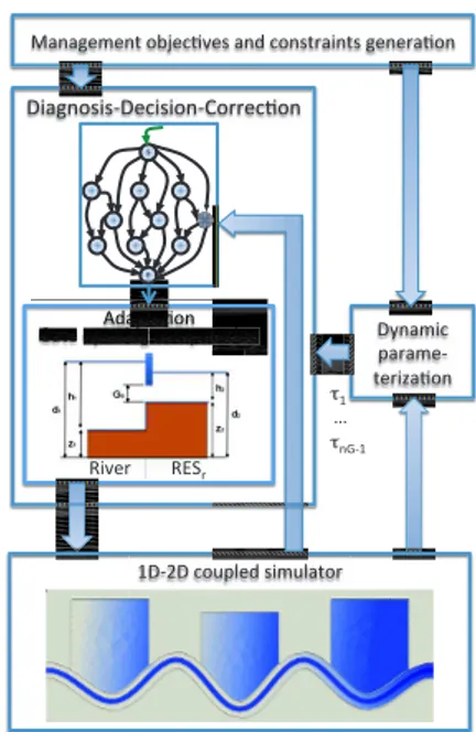
Figure 3 – Simulator and supervisory control scheme
3 IMPLEMENTATION AND RESULTS
3.1 Implementation
In order to evaluate the efficiency of the proposed model, a simulation for several cases of flood was done. A test case river was used and the implemen-tation of this river was performed by using a 1D-2D coupled numerical model according to the descrip-tion given in (Garcia-Navarro et al., 2008;
Morales-Hernandez et al., 2012; Morales-Hern´andez et al.,
2013). 1D and 2D models are formulated using a con-servative upwind cell-centred finite volume scheme. The discretization was based on cross-sections for the 1D model and with triangular unstructured grid for the 2D model. Coupling techniques were based on mass and momentum conservation. The cross section geometry and topography was derived from the Ebro river, however, the shape of the river was simplified. As summarized in Figure 3, the process and SCADA systems were replaced by a 1D-2D coupled simula-tor (developed by (Garcia-Navarro et al., 2008)). In the 1D-2D coupled simulator, each gate is modeled considering that the flow discharge that crosses the gate is governed by the difference between the water level in both side of the gate. The 1D-2D coupled simulator entries are the values of the gate opening thus, the Adaptation Block consisted in the compu-tation of the gate opening values from the optimal flow, by means of a static inversion of the free flow open channel equations (Litrico et al., 2008). The Dynamic Parameterization block was used in order to
compute the time delays at each kTc (k = 1, · · · , n).
The transfer time, τr, from the gate Gr to the gate
Gr+1, r = 1, · · · , nGwas approximated by the
exam-Algorithm 4: Actualization TM and Simulator
input :
nG the number of gates and FCR in the system
T M the n × 2nG temporization matrix
k the iteration number
kr= ⌊Tτr
c⌋, r = 1, · · · , nG− 1
Vmes
RESr(k) the measured amount of water
stored in the RESrat kTc
Qmes
(Gr,RESr)(k) the measured discharge from
gate Gr to RESrat kTc
Gthe network
output:
T M the n × 2nG temporization matrix
begin forr = 1 to nG− 1 do T M (k + kr, r + 1) ← T M (k + kr− 1, r + 1) + ϕ∗GrP0(k) + max(0, ϕ∗ GrRESr(k) − Q mes (Gr,RESr)(k)) end forr = 1 to nG− 1 do T M (k + 1, nG+ r) ← T M (k, nG+ r) + VRESmesr(k) end end ple): τr= QGr S.dGr,Gr+1 (2)
where QGr is the discharge measured at gate Gr, S
is the wetted cross section, and dGr,Gr+1 is the
dis-tance traveled from Grto Gr+1. In order to evaluate
time delays, methods such as the ones developed in (Romera et al., 2013) or in (Bautista and Clemmens, 2015) can also be used. The values measured with the simulator were introduced in the algorithm for actualization of temporized matrix, as described in algorithm 4.
3.2 Performance criteria
The flood wave attenuation can be defined as the de-crease in the downstream peak flow, due to the atten-uation of the flood (Bedient, P. B. et al., 2013). In order to evaluate the performances of the proposed flood attenuation method, three indicators were de-fined : the attenuation rate (AR), the rate of filling (RF) and the attenuation wave rate (AWR). These measures allow us to evaluate how we prevent down-stream flood risk by using the proposed method. All these measures are computed over the time horizon
Hf, i. e. for k = 0, · · · , n; and we denote Qout the
downstream flow. The AR permits to measure the difference between the attenuation threshold objec-tive and the obtained attenuation threshold. It is defined as the ratio between the mean effective
at-tenuation flow, Qmea, and the predefined attenuation
flow Qlam, as given in equation (3) and equation (4).
AR = Qmea Qlam (3)
if ∃k|Qout(k) > Qlam Qmea= mean
Qout(k)>Qlam
Qout(k)
else Qmea= max
k=1···nQout(k)
(4) Another estimator of the attenuation capacity is the AWR which compares the case where the gates are al-ways closed to the case in which a strategy is involved and is expressed by equation (5).
AW R = P Qcg(k)>Qlam Qcg(k) − P Qout(k)>Qlam Qout(k) P Qcg(k)>Qlam Qcg(k) (5) The downstream flow when the gates are closed is
denoted Qcg. Finally, RF indicates the water volume
storage efficiency. It is computed as the ratio between
the water volume stored in all the reservoirs, Vs, and
the estimated water volume to be stored, Vlam, as
in-dicated in equation (6), and assuming that VRESr is
the maximum volume stored in the reservoir RESr
(r = 1, · · · , nG), during the time horizon Hf. Vlamis
approximated by the trapezoidal numerical
integra-tion of the input flow, Qinput, above Qlam.
RF = Vs Vlam , Vs= nG X r=1 VRESr (6) 3.3 Results
Simulation were done within the horizon Hf =
86400s corresponding to 24 hours, Tc = 100s thus
n = 864. The simulated river was equipped with
nG = 3 flood control reservoirs, each one controlled
by a gravitational gate.
The first case studied is a flood episode with one peak
flow of 790.31m3/s occurring at k = 330 i. e. around
9 hours after the beginning of the simulation. The values of attenuation and draw-off flows were set to
Qlam = 675m3/s and Qdo = 600m3/s ≈ 90%Qlam.
For this one peak flood, the measured time delays
var-ied between 11Tcand 16Tc as illustrated in Figure 4.
Thus in order to compare the results obtained when the strategy involved constant time delay or varying time delay, we realized simulation for constant time
delays underestimated or overvalued: τ1= τ2= 10Tc,
τ1 = τ2 = 11Tc, τ1 = τ2 = 14Tc, τ1 = τ2 = 16Tc,
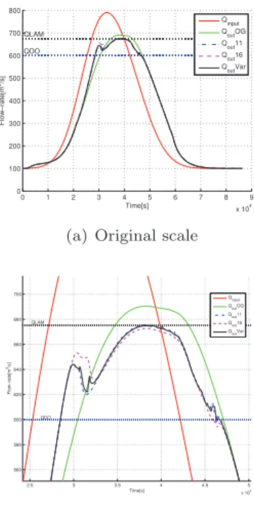
τ1= τ2= 18Tc. In Figure 5, the Qinput value is given
Figure 4 – τ1and τ2evolution for a 1-peak simulation
with Qlam= 675m3/s and Qdo= 600m3/s.
are compared. Case one, the gates always open (un-regulated reservoirs) is given in green. Case two, the proposed strategy applied with constant time delays:
τ1 = τ2 = 11Tc is given in blue. Case three, the
proposed strategy applied with constant time delays:
τ1 = τ2 = 16Tc is given in magenta. Case four, the
proposed strategy applied with varying time delays, expressed as function of flow and computed thanks to the Dynamic Parameterization block is given in black. When the gate are always open, the peak flood is
re-duced however, the discharge exceeds the Qlamvalue.
When time delays are computed, the Qout curve is
between the Qoutcurves obtained for the time delays
set to their variation interval bounds. In all these
cases, the Qout maximum value is given, and denoted
Qmax in the second column of the Table 1.
With-out the use of flood control reservoirs the peak flow
reaches 777.08m3/s, when the gates are always open,
the peak flow reaches 690.39m3/s. When the
pro-posed strategy is applied, the peak flow decreases and
it is lower than the Qlam value when the time delays
are computed. When time delays are set to constant values, performance decreases, and we can conclude that it is preferred to overestimate the time delays.
Case Qmax AR% AWR% RF%
Open Gates 690.39 101.65 36.83 123.42 τr= 10Tc 679.26 100.39 65.09 115.80 τr= 11Tc 675.46 100.05 91.12 112.99 τr= 14Tc 673.83 99.83 100 112.21 τr= 16Tc 672.64 99.65 100 111.65 τr= 18Tc 675.47 100.04 90.45 113.94 Varying τ 674.92 99.99 100 112.59
Table 1 – AR, AWR and RF values for the 1 peak scenario.
The values of the performance criteria obtained in the studied cases are given in Table 1. Whatever the method used for the time delays computation, the ability to absorb the flood is increased when
us-ing the transportation network. Indeed AW R =
65.09% when the time delays are underestimated, and AW R = 90.45% when the time delays are overvalued. When the time delays are set to the minimum value of their variation interval AW R = 91.12%. When the time delays are computed or set to values high
0 1 2 3 4 5 6 7 8 9 x 10⁴ 0 100 200 300 400 500 600 700 800 QLAM QDO Time[s] Flow−rate[m 3/s] Qinput Q outOG Qout11 Qout16 Q outVar
(a) Original scale
2.5 3 3.5 4 4.5 5 x 10⁴ 560 580 600 620 640 660 680 700 QLAM QDO Time[s] Flow−rate[m 3/s] Q input QoutOG Qout11 Qout16 QoutVar (b) Zoom
Figure 5 – Qinput and Qout for a 1-peak simulation
with Qlam= 675m3/s and Qdo= 600m3/s.
enough, AW R = 100%, the peak flow is under the
Qlam value. Finally, AW R = 36.83% when the gates
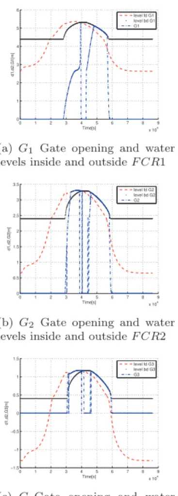
are not regulated. AR value is better if it is as close as possible to 100% which is the case for computed time delays. Finally, in all cases the water stored in the reservoir is upper than the estimated needed volume. The gates’ opening height computed by the algorithm with varying time delays is given in blue in Figure 6(a)
for the gate G1, in Figure 6(b) for the gate G2 and
in Figure 6(c) for the gate G3. The water level inside
the reservoir is represented in black and the water level in the river in front of the gates in red. The water levels are measured with regard to the river bed. In each Figure, the gate is first opened in order to store water, thereafter, during the phase when the
discharge is between Qlam and Qdo the gate is closed
and finally, the gate is opened in order to empty the reservoir.
In the fourth illustrated cases, the water level inside the reservoirs is superimposed in Figure 7(a) for the
gate G1, in Figure 7(b) for the gate G2and in Figure
7(c) for the gate G3. The always open gates case is
given in green. The proposed strategy applied with
constant time delays: τ1 = τ2 = 11Tc is given in
blue, with τ1= τ2= 16Tc in magenta and with
vary-ing time delays in black. For each one of the three gates, the green curve is always above the other ones, which indicates that the needed reservoirs’ capacity is lower when using the regulation scheme. Moreover, the reservoirs are filled later in that case and the wa-ter remains less time in the reservoirs, thus the
agri-0 1 2 3 4 5 6 7 8 9 x 10⁴ 0 1 2 3 4 5 6 Time[s] d1,d2,G1[m] level fd G1 level bd G1 G1
(a) G1 Gate opening and water
levels inside and outside F CR1
0 1 2 3 4 5 6 7 8 9 x 10⁴ 0 0.5 1 1.5 2 2.5 3 3.5 Time[s] d1,d2,G2[m] level fd G2 level bd G2 G2
(b) G2 Gate opening and water
levels inside and outside F CR2
0 1 2 3 4 5 6 7 8 9 x 10⁴ −1.5 −1 −0.5 0 0.5 1 1.5 Time[s] d1,d2,G3[m] level fd G3 level bd G3 G3
(c) G3Gate opening and water
levels inside and outside F CR3
Figure 6 – Gate opening and water levels for a
1-peak simulation with Qlam = 675m3/s and Qdo =
600m3/s. The water levels inside (outside) the
reser-voirs are denoted bd (fd) respectively.
cultural zone are better preserved. The water level curve in the case of computed time delays is between the curves obtained for the time delays set to their variation interval bounds.
The second case studied is a flood episode with two
peak flows, the first one is of 838.79m3/s occurring
at k = 324 i. e. around 9 hours after the beginning
of the simulation, the second is of 753.79m3/s and
occurs at k = 570 i. e. around 16 hours after the beginning of the simulation. The values of
attenua-tion and draw-off flows were set to Qlam = 710m3/s
and Qdo = 680m3/s ≈ 95%Qlam. This case was
pro-posed in order to evaluate the ability of the method
to attenuate a second flood episode. Moreover, Qdo
is set high enough to allow for a water draw-off from the reservoir after the first peak and before the sec-ond one and so that the ability to absorb the secsec-ond flood exists. Because results obtained in the one peak flood episode shown that results were better in the computed time delay case, we compared for the two peaks flood episode only this case and the case when gates are always open. For this two peak flood, the
0 1 2 3 4 5 6 7 8 9 x 10⁴ 4.4 4.5 4.6 4.7 4.8 4.9 5 5.1 5.2 5.3 5.4 Time[s]
Water level in the first reservoir [m]
OG tau 11 tau 16 tau Var
(a) Fist reservoir
0 1 2 3 4 5 6 7 8 9 x 10⁴ 2.2 2.4 2.6 2.8 3 3.2 3.4 3.6 Time[s]
Water level in the second reservoir [m]
OG tau 11 tau 16 tau Var (b) Second reservoir 0 1 2 3 4 5 6 7 8 9 x 10⁴ 0.4 0.5 0.6 0.7 0.8 0.9 1 1.1 1.2 1.3 Time[s]
Water level in the third reservoir [m]
OG tau 11 tau 16 tau Var
(c) Thrid reservoir
Figure 7 – Comparison of water levels inside the
reser-voirs for a 1-peak simulation with Qlam = 675m3/s
and Qdo = 600m3/s. 0 1 2 3 4 5 6 7 8 9 x 10⁴ 1000 1100 1200 1300 1400 1500 1600 1700 Times[s] Tranfer time [s] G1−G2 G2−G3
Figure 8 – τ1and τ2evolution for a 2-peaks simulation
with Qlam= 710m3/s and Qdo= 680m3/s.
measured time delays varied between 11Tc and 16Tc
as illustrated in Figure 8.
In Figure 9, the Qinput value is given in red, the
al-ways open gates case in green. The proposed strat-egy applied with varying time delays is given in black. When the gate are always open, the peak flood is
re-duced however, the discharge exceeds the Qlamvalue.
When time delays are computed, the Qout curve is
between the Qout curves obtained for the time
de-lays set to their variation interval bounds. With-out the use of flood control reservoirs the peak flow
reaches 823.01m3/s for the first wave and 746.19m3/s
for the second one. When applying the strategy, the
0 2 4 6 8 10 12 x 104 0 100 200 300 400 500 600 700 800 900 QLAM QDO Time[s] Flow−rate[m 3/s] Qinput Q outOG QoutVar
(a) Original scale
2 2.5 3 3.5 4 4.5 5 5.5 6 6.5 7 x 10⁴ 560 580 600 620 640 660 680 700 720 740 760 QLAM QDO Time[s] Flow−rate[m 3/s] Qinput QoutOG Q outVar (b) Zoom
Figure 9 – Qinput and Qout for a 2-peak simulation
with Qlam= 710m3/s and Qdo= 680m3/s.
712.56m3/s for the second one. Applying the
strat-egy allows the discharge to remain under the Qlam
value for the first wave and very close to it for the second wave. The values of the performance criteria
Case AR% AWR% RF%
1st pic 2nd pic
Open Gates 100.76 64.34 77.34 103.17
Varying τ 100.16 100 91.90 99.07
Table 2 – AR, AWR and RF values for the 2 peaks scenario in the two different cases.
computed for each case are given in Table 2. As in the first test, the ability to absorb the both flood waves is increased when using the proposed method. Indeed, for the first wave, AW R = 100% when gates are reg-ulated whereas AW R = 64.34% when gates are not regulated. For the second wave AW R = 91.90% when the strategy is used whereas AW R = 77.34% when the gates remain open. Before the arrival of the sec-ond flood, we take advantage of the decrease of the water level in the river to release a certain amount of water from FCRs in the river. This enables us to better accommodate the second wave of flooding.
4 CONCLUSION
In this paper, we propose a supervisory control scheme for the management of a river section in a flood situation. The Diagnosis-Detection-Correction block is based on a transportation network
model-ing includmodel-ing time delay. It permits to account for the variation of time delays without any modification in the network structure. The results of the connec-tion between the method and the 1D-2D-coupled river simulator were displayed, highlighting the benefits of the strategy. The proposed simulated case permit-ted to attest the feasibility of including varying time delays in the network. Results are expected to be most obvious when considering a more extended net-work with longer delays. The strategy consists of two phases: water storage and water release. The storage phase keeps the flow below the attenuation discharge threshold imposed: the flood is attenuated, and the draw-off phase, enables us to preserve the floodplain. The strategy can be used in order to estimate the ca-pability of river systems equipped with flood control reservoirs to control floods. One of the most impor-tant problem to be studied, beyond quantitative flood management, is the quality of water in the river and in the reservoirs. Future research will focus on the integration of pollution problems into the strategy. ACKNOWLEDGMENTS
The authors want to thank Confederaci´on Hidrogr´a-fica del Ebro for providing the case study used in this paper as well as for sharing their hydrological man-agement expertise, Fluid Mechanics, LIFTEC-EINA, University of Zaragoza for providing the 1D-2D cou-pled simulator.
REFERENCES References
Amin, S.; Litrico, X.; Sastry, S.; Bayen, AM., Sept. 2013a. Cyber Security of Water SCADA Systems -Part I: Analysis and Experimentation of Stealthy Deception Attacks, IEEE Transactions on Control Systems Technology 21 (5), 1963–1970.
Amin, S.; Litrico, X.; Sastry, S.; Bayen, AM., Sept. 2013b. Cyber Security of Water SCADA Systems - Part II: Attack Detection Using Enhanced Hy-drodynamic Models, IEEE Transactions on Control Systems Technology 21 (5), 1679–1693.
Bautista E. and Clemmens A. J., Dec. 2005. Vol-ume Compensation Method for Routing Irrigation Canal Demand Changes, Journal of Irrigation and Drainage Engineering, 131 (6), 494–503.
Bedient, P. B., Huber, W. C., Vieux, B. E., 2013. Hy-drology and floodplain analysis, 5th Edition. Pren-tice Hall, Upper Saddle River, New Jersey, USA. Cheng, C., Chau, K. W., Oct. 2001. Fuzzy iteration
methodology for reservoir flood control operation. Journal of the American Water Resources Associ-ation 37 (5), 1381–1388.
Chuntian, C., Chau, K., Nov. 2002. Three-person multi-objective conflict decision in reservoir flood control. European Journal of Operational Research 142 (3), 625–631.
Duviella, E., Rajaoarisoa, L., Blesa, J., Chuquet, K., June 2013. Adaptive and predictive control architecture of inland navigation networks in a global change context: application to the Cuinchy-Fontinettes reach. In: 7th IFAC Conference on Manufacturing Modelling, Management, and Con-trol, (MIM). IFAC, Saint Petersburg, Russia, pp. 2201–2206.
Figueiredo, J., Ayala Botto, M., Rijo, M., 2013. SCADA system with predictive controller applied to irrigation canals. Control Engineering Practice 21 (6), 870–886.
Fu, G., 2008. A fuzzy optimization method for mul-ticriteria decision making: An application to reser-voir flood control operation. Expert Systems with Applications 34, 145–149.
Garcia-Navarro, P., Brufau, P., Burguete, J., Murillo, J., 2008. The shallow water equations: An exam-ple of hyperbolic system. Monografias de la Real Academia de Ciencias de Zaragoza 31, 89–119. Karamouz, M., Szidarovszky, F., Zahraie, B., 2003.
Water Resources Systems Analysis. Lewis Publish-ers, New York, USA.
Karbowski, A., Malinowski, K., Niewiadomska-Szynkiewicz, E., Jan. 2005. A hybrid analytic/rule-based approach to reservoir system management during flood. Decision Support Systems 38 (4), 599–610.
Litrico, X., Malaterre, P., Baume, J.-P., Ribot-Bruno, J. E., 2008. Conversion from discharge to gate opening for the control of irrigation canals. Jour-nal of Irrigation and Drainage Engineering 134 (3), 305–314.
Mora, D., Taisch, M., Colombo, A. W., Mendes, J. M., Jul. 2012. Service-Oriented Architecture ap-proach for Industrial ”System of Systems”: State-of-the-Art for Energy Management. In: 2012 10th IEEE International Conference on Industrial Infor-matics, (INDIN). IEEE, Beijing, China, pp. 1246– 1246.
Morales-Hern´andez, M., Garc´ıa-Navarro, P.,
Bur-guete, J., Brufau, P., Apr. 2013. A conservative strategy to couple 1D and 2D models for shallow water flow simulation. Computers & Fluids to ap-pear.
Morales-Hernandez, M., Garc´ıa-Navarro, P., Murillo, J., Aug. 2012. A large time step 1D upwind ex-plicit scheme (CF L > 1): Application to shallow
water equations. Journal of Computational Physics 231 (19), 6532–6557.
Nagesh Kumar, D., Baliarsingh, F., Srinivasa Raju, K., Jul. 2009. Optimal Reservoir Operation for Flood Control Using Folded Dynamic Program-ming. Water Resources Management 24 (6), 1045– 1064.
Needham, J. T., Watkins Jr., D. W., Lund, J. R., Nanda, S. K., 2000. Linear Programming For Flood Control In The Iowa And Des Moines Rivers. Jour-nal Of Water Resources Planning And Manage-ment 126 (3), 118–127.
Nouasse, H., Charbonnaud, P., Chiron, P., Murillo, J., Morales, M., Garcia-Navarro, P., Perez, G., Jul. 2012. Flood lamination strategy based on a three-flood-diversion-area system management. In: 2012 20th Mediterranean Conference on Control & Au-tomation (MED). IEEE, Barcelona, pp. 866–871. Nouasse, H., Chiron, P., Archim`ede, B., 2013. A flood
lamination strategy based on transportation net-work with time delay. Water Science & Technology 68 (8), 1668–1696.
Nouasse, H., Chiron, P., Archim`ede, B., Sept. 2013. A water storage and release strategy for flood management based on transportation net-work with time delay. In: 2013 IEEE 18th Confer-ence on Emerging Technologies Factory Automa-tion (ETFA). IEEE, Cagliari, Italy, pp. 1–8. Pfitscher, L.L., Bernardon, D.P., Kopp, L. M.,
Heck-ler, M. V T, Behrens, J., Montani, P.B., Thome, B., 2012. Automatic control of irrigation systems aiming at high energy efficiency in rice crops. In: 2012 8th International Caribbean Conference on Devices, Circuits and Systems (ICCDCS). IEEE, Playa del Carmen, Mexico, pp. 1–4.
Puerto, P., Domingo, R., Torres, R., Perez-Pastor, A., Garcia-Riquelme, M., 2013. Remote manage-ment of deficit irrigation in almond trees based on maximum daily trunk shrinkage. Water relations and yield. Journal of Agricultural Water Manage-ment 126, 33–45.
Ratnayake, U., Harboe, R., 2007. Deterministic and Stochastic Optimization of a Reservoir System. In-ternational Water Resources Association 32 (1), 155–162.
Romera, J., Ocampo-Martinez, C., Puig, V.,
Quevedo, J., 2013. Flooding management using hy-brid model predictive control: application to the Spanish Ebro River. Journal of Hydroinformatics 15 (2), 366–380.