Support Vector Machine Versus Random Forest for Remote Sensing Image Classification: A Meta-Analysis and Systematic Review.

(1)

> REPLACE THIS LINE WITH YOUR PAPER IDENTIFICATION NUMBER (DOUBLE-CLICK HERE TO EDIT) < 1

Abstract—Several machine-learning algorithms have been proposed for remote sensing image classification during the past two decades. Among these machine learning algorithms, Random Forest (RF) and Support Vector Machines (SVM) have drawn attention to image classification in several remote sensing applications. This paper reviews RF and SVM concepts relevant to remote sensing image classification and applies a meta-analysis of 251 peer-reviewed journal papers. A database with more than 40 quantitative and qualitative fields was constructed from these reviewed papers. The meta-analysis mainly focuses on: (1) the analysis regarding the general characteristics of the studies, such as geographical distribution, frequency of the papers considering time, journals, application domains, and remote sensing software packages used in the case studies, and (2) a comparative analysis regarding the performances of RF and SVM classification against various parameters, such as data type, RS applications, spatial resolution, and the number of extracted features in the feature engineering step. The challenges, recommendations, and potential directions for future research are also discussed in detail. Moreover, a summary of the results is provided to aid researchers to customize their efforts in order to achieve the most accurate results based on their thematic applications.

Index Terms— Random Forest, Support Vector Machine, Remote Sensing, Image classification, Meta-analysis.

I. INTRODUCTION

ecent advances in Remote Sensing (RS) technologies, including platforms, sensors, and information infrastructures, have significantly increased the accessibility to the Earth Observations (EO) for geospatial analysis [1]–[5]. In addition, the availability of high-quality data, the temporal frequency, and comprehensive coverage make them

M. Sheykhmousa is with the OpenGeoHub (a not-for-profit research foundation), Agro Business Park 10, 6708 PW Wageningen, The Netherlands (e-mail: mohammadreza.sheykhmousa@opengeohub.org).

M. Mahdianpari (corresponding author) is with the C-CORE, 1 Morrissey Rd, St. John’s, NL A1B 3X5, Canada and Department of Electrical and Computer Engineering, Faculty of Engineering and Applied Science, Memorial University of Newfoundland, St. John’s, NL A1B 3X5, Canada (e-mail: m.mahdianpari@mun.ca).

H. Ghanbari is with the Department of geography, Université Laval, Québec, QC G1V 0A6, Canada (e-mail: hamid.ghanbari.1@ulaval.ca).

F. Mohammadimanesh is with the the C-CORE, 1 Morrissey Rd, St. John’s, NL A1B 3X5, Canada (e-mail: fariba.mohammadimanesh@c-core.ca). P. Ghamisi is with the Helmholtz-Zentrum Dresden-Rossendorf (HZDR), Helmholtz Institute Freiberg for Resource Technology (HIF), Division of "Exploration Technology", Chemnitzer Str. 40, Freiberg, 09599 Germany (e-mail: p.ghamisi@gmail.com).

S. Homayouni is with the Institut National de la Recherche Scientifique (INRS), Centre Eau Terre Environnement, Quebec City, QC G1K 9A9, Canada (e-mail: saeid.homayouni@ete.inrs.ca).

advantageous for several agro-environmental applications compared to the traditional data collections approaches [6]– [8]. In particular, land use and land cover (LULC) mapping is the most common application of RS data for a variety of environmental studies, given the increased availability of RS image archives [9]–[13]. The growing applications of LULC mapping alongside the need for updating the existing maps have offered new opportunities to effectively develop innovative RS image classification techniques in various land management domains to address local, regional, and global challenges [14]–[21].

The large volume of RS data [15], the complexity of the landscape in a study area [22]–[24], as well as limited and usually imbalanced training data [25]–[28], make the classification a challenging task. Efficiency and computational cost of RS image classification [29] is also influenced by different factors, such as classification algorithms [30]–[33], sensor types [34]–[37], training samples [38]–[41], input features [42]–[46], pre- and post-processing techniques [47], [48], ancillary data [49], [50], target classes [22], [51], and the accuracy of the final product [21], [50], [52]–[54]. Accordingly, these factors should be considered with caution for improving the accuracy of the final classification map. Carrying a simple accuracy assessment, through the Overall Accuracy (OA) and Kappa coefficient of agreement (K), by the inclusion of ground truth data might be the most common and reliable approach for reporting the accuracy of thematic maps. These accuracy measures make the classification algorithms comparable when independent training and validation data are incorporated into the classification scheme [31], [55]–[57], [57].

Given the development and employment of new classification algorithms, several review articles have been published. To date, most of these reviews on remote sensing classification algorithms have provided useful guidelines on the general characteristics of a large group of techniques and methodologies. For example, [58] represented a meta-analysis of the popular supervised object-based classifiers and reported the classification accuracies with respect to several influential factors, such as spatial resolution, sensor type, training sample size, and classification approach. Several review papers also demonstrated the performance of the classification algorithms for a specific type of application. For instance, [59] summarized the significant trends in remote sensing techniques for the classification of tree species and discussed the effectiveness of different sensors and algorithms for this

Support Vector Machine vs. Random Forest for Remote

Sensing Image Classification: A Meta-analysis and

systematic review

Mohammadreza Sheykhmousa, Masoud Mahdianpari, Member, IEEE, Hamid Ghanbari, Fariba Mohammadimanesh, Pedram Ghamisi, Senior Member, IEEE, and Saeid Homayouni, Senior Member, IEEE

(2)

application. The developments in methodologies for processing a specific type of data is another dominant type of review papers in remote sensing image classification. For example, [60] reviews the usefulness of high-resolution LiDAR sensor and its application for urban land cover classification, or in [7], an algorithmic perspective review for processing of hyperspectral images is provided.

Over the past few years, deep learning algorithms have drawn attention for several RS applications [33], [61], and as such, several review articles have been published on this topic. For instance, three typical models of deep learning algorithms, namely deep belief network, convolutional neural networks, and stacked auto-encoder, were analyzed in [62]. They also discussed the most critical parameters and the optimal configuration of each model. Studies, such as [63] who compared the capability of deep learning architectures with Support Vector Machine (SVM) for RS image classification, and [64] who focused on the classification of hyperspectral data using deep learning techniques, are other examples of RS deep learning review papers.

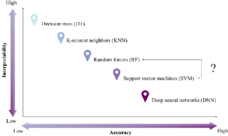
The commonly employed classification algorithms in the remote sensing community include support vector machines (SVMs) [65], [66], ensemble classifiers, e.g., random forest (RF) [10], [67], and deep learning algorithms [30], [68]. Deep learning methods has the ability to retrieve complex patterns and informative features from the satellite image data. For example, CNN has shown performance improvements over SVM and RF [69]–[71]. However, one of the main problems with deep learning approaches is their hidden layers; “black box” [61] nature, which results in the loss of interpretability (see Fig. 1). Another limitation of a deep learning models is that they are highly dependent on the amount of training data i.e., ground truth. Moreover, implementing CNN required expert knowledge and computationally is expensive and needs dedicated hardware to handle the process. On the other hand, recent researches show SVM and RF (i.e., relatively easily implementable methods) can handle learning tasks with a small amount of training dataset, yet demonstrate competitive results with CNNs [72]. Deep learning methods have the ability to retrieve complex patterns and informative features from the satellite imagery. For example, CNN has shown performance improvements over SVM and RF [69], [70]. However, one of the main problems with deep learning approaches is their hidden layers; “black box” nature [61], which results in the loss of interpretability (see Fig. 1). Another limitation of deep learning models is that they are highly dependent on the availability of abundant high quality ground truth data. Moreover, implementing CNN requires expert knowledge and it is computationally expensive and needs dedicated hardware to handle the process. On the other hand, recent researches show SVM and RF (i.e., relatively easily implementable methods) can handle learning tasks with a small amount of training dataset, yet demonstrate competitive results with CNNs [72]. Although there is an ongoing shift in the application of deep learning in RS image classification, SVM and RF have still held the researchers’ attention due to lower computational complexity and higher

interpretability capabilities compared to deep learning models. More specifically, SVM maintenance among the top classifiers is mainly because of its ability to tackle the problems of high dimensionality and limited training samples [73], while RF holds its position due to ease of use (i.e., does not need much hyper-parameter fine-tuning) and its ability to learn both simple and complex classification functions [74], [75]. As a result, the relatively high similar performance of SVM and RF in terms of classification accuracies make them among the most popular machine learning classifiers within the RS community [76]. As a result, giving merit to one of them is a difficult task as past comparison-based studies, as well as some review papers, provide readers with often contradictory conclusions, which was somehow confusing. For instance, [74] reported SVMs can be considered the “best of class” algorithms for classification; however, [75], [77] suggested that RF classifiers may outperform support vector machines for RS image classification. This knowledge gap was identified in the field of bioinformatics and filled by an exclusive review of RFs vs. SVMs [78]; however, no such a detailed survey is available for RS image classification.

Table I summarizes the review papers on recent classification algorithms of remote sensing data, where a large part of the literature is devoted to RFs or is discussed as an alternative classifier. The majority of these review papers are descriptive and do not offer a quantitative assessment of the stability and suitability of RF and SVM classification algorithms. Accordingly, the general objective of this study is to fill this knowledge gap by comparing RF and SVM classification algorithms through a meta-analysis of published papers and provide remote sensing experts with a “big picture” of the current research in this field. To the best of the authors knowledge, this is the first study in the remote sensing filed that provides a one to one comparison analysis for RF and SVM in various remote sensing applications.

To fulfill the proposed meta-analysis task, more than 250 peer-reviewed papers have been reviewed in order to construct a database of case studies that include RFs and SVMs either in one-to-one comparison or individually with other machine learning methods in the field of remote sensing image classification.

Fig. 1. Interpretability-accuracy trade-off in machine learning classification algorithms.

(3)

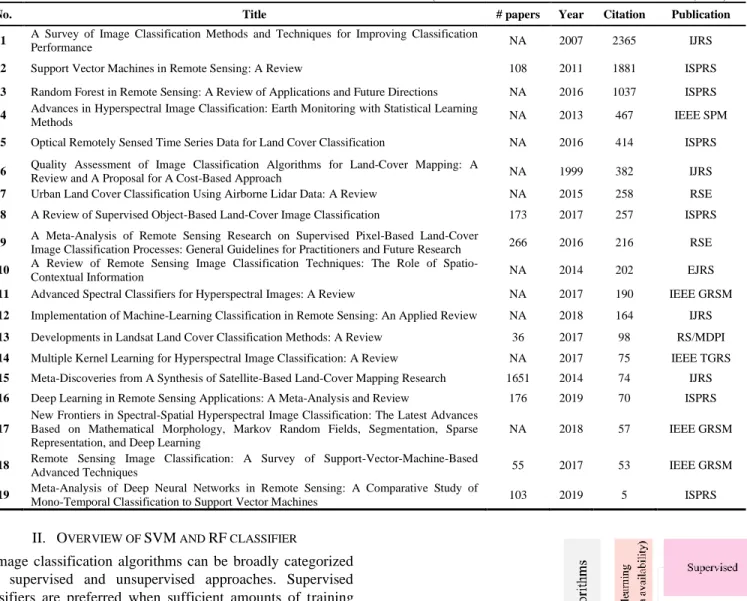
TABLEI.SUMMARY OF RELATED SURVEYS ON REMOTE SENSING IMAGE CLASSIFICATION (THE NUMBER OF CITATIONS IS REPORTED BY APRIL 20,2020).

No. Title # papers Year Citation Publication

1 A Survey of Image Classification Methods and Techniques for Improving Classification

Performance NA 2007 2365 IJRS

2 Support Vector Machines in Remote Sensing: A Review 108 2011 1881 ISPRS

3 Random Forest in Remote Sensing: A Review of Applications and Future Directions NA 2016 1037 ISPRS

4 Advances in Hyperspectral Image Classification: Earth Monitoring with Statistical Learning

Methods NA 2013 467 IEEE SPM

5 Optical Remotely Sensed Time Series Data for Land Cover Classification NA 2016 414 ISPRS

6 Quality Assessment of Image Classification Algorithms for Land-Cover Mapping: A _{Review and A Proposal for A Cost-Based Approach} NA 1999 382 IJRS

7 Urban Land Cover Classification Using Airborne Lidar Data: A Review NA 2015 258 RSE

8 A Review of Supervised Object-Based Land-Cover Image Classification 173 2017 257 ISPRS

9 A Meta-Analysis of Remote Sensing Research on Supervised Pixel-Based Land-Cover

Image Classification Processes: General Guidelines for Practitioners and Future Research 266 2016 216 RSE

10 A Review of Remote Sensing Image Classification Techniques: The Role of

Spatio-Contextual Information NA 2014 202 EJRS

11 Advanced Spectral Classifiers for Hyperspectral Images: A Review NA 2017 190 IEEE GRSM

12 Implementation of Machine-Learning Classification in Remote Sensing: An Applied Review NA 2018 164 IJRS

13 Developments in Landsat Land Cover Classification Methods: A Review 36 2017 98 RS/MDPI

14 Multiple Kernel Learning for Hyperspectral Image Classification: A Review NA 2017 75 IEEE TGRS

15 Meta-Discoveries from A Synthesis of Satellite-Based Land-Cover Mapping Research 1651 2014 74 IJRS

16 Deep Learning in Remote Sensing Applications: A Meta-Analysis and Review 176 2019 70 ISPRS

17

New Frontiers in Spectral-Spatial Hyperspectral Image Classification: The Latest Advances Based on Mathematical Morphology, Markov Random Fields, Segmentation, Sparse Representation, and Deep Learning

NA 2018 57 IEEE GRSM

18 Remote Sensing Image Classification: A Survey of Support-Vector-Machine-Based

Advanced Techniques 55 2017 53 IEEE GRSM

19 Meta-Analysis of Deep Neural Networks in Remote Sensing: A Comparative Study of

Mono-Temporal Classification to Support Vector Machines 103 2019 5 ISPRS

II. OVERVIEW OF SVM AND RF CLASSIFIER

Image classification algorithms can be broadly categorized into supervised and unsupervised approaches. Supervised classifiers are preferred when sufficient amounts of training data are available. Parametric and non-parametric methods are another categorization of classification algorithms based on data distribution assumptions (see Fig. 2). Yu et al. [79] reviewed 1651 articles and reported that supervised parametric algorithms were the most frequently used technique for remote sensing image classification. For example, the maximum likelihood (ML) classifier, as a supervised parametric approach, was employed in more than 32% of the reviewed studies. Supervised non-parametric algorithms, such as SVM and ensemble classifiers, obtained more accurate results, yet they were less frequently used compared to supervised parametric methods [79].

Prior to the introduction of Random Forest (RF), Support Vector Machine (SVM) has been in the spotlight for RS image classification, given its superiority compared to Maximum Likelihood Classifier (MLC), K-Nearest Neighbours (KNN), Artificial Neural Networks (ANN), and Decision Tree (DT) for RS image classification. Since the introduction of RF, however, it has drawn attention within the remote sensing community, as it produced classification accuracies comparable with those of SVM [75], [76]. An overview of SVM and RF classification algorithms has been presented in the following sections.

Fig. 2. A Taxonomy of Image classification algorithms.

A. Support Vector Machine Classifier

The Support vector machines algorithm, introduced firstly in the late 1970s by Vapnik and his group, is one of the most widely used kernel-based learning algorithms in a variety of machine learning applications, and especially image classification [74]. In SVMs, the main goal is to solve a convex quadratic optimization problem for obtaining a globally optimal solution in theory and thus, overcoming the local extremum dilemma of other machine learning techniques. SVM belongs to non-parametric supervised techniques, which are insensitive to the distribution of

(4)

underlying data. This is one of the advantages of SVMs compared to other statistical techniques, such as maximum likelihood, wherein data distribution should be known in advance [76].

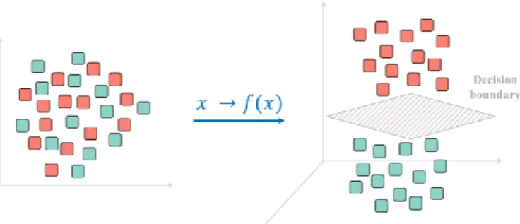
SVM, in its basic form, is a linear binary classifier, which identifies a single boundary between two classes. The linear SVM assumes the multi-dimensional data are linearly separable in the input space (see Fig. 3). In particular, SVMs determine an optimal hyperplane (a line in the simplest case) to separate the dataset into a discrete number of predefined classes using the training data. To maximize the separation or margin, SVMs use a portion of the training sample that lies closest in the feature space to the optimal decision boundary, acting as support vectors [80]–[83]. These samples are the most challenging data to classify and have a direct impact on the optimum location of the decision boundary [38], [76]. The optimal hyperplane, or the maximal margin, can be mathematically and geometrically defined. It refers to a decision boundary that minimizes misclassification errors attained during the training step [66], [67]. As seen in Fig. 3, a number of hyperplanes with no sample between them are selected, and then the optimal hyperplane is determined when the margin of separation is maximized [76], [77]. This iterative process of constructing a classifier with an optimal decision boundary is described as the learning process [79].

Fig. 3. An SVM example for linearly separable data.

In practice, the data samples of various classes are not always linearly separable and have overlap with each other (see Fig. 4). Thus, linear SVM can not guarantee a high accuracy for classifying such data and needs some modifications. Cortes and Vapnik [80] introduced the soft margin and kernel trick methods to address the limitation of linear SVM. To deal with non-linearly separable data, additional variables (i.e., slack variables) can be added to SVM optimization in the soft margin approach. However, the idea behind the kernel trick is to map the feature space into a higher dimension (Euclidean or Hilbert space) to improve the separability between classes [86], [87]. In other words, using the kernel trick, an input dataset is projected into a higher dimensional feature space where the training samples will become linearly separable.

Fig. 4. An SVM example for non-linearly separable data with the kernel trick.

The performance of SVM largely depends on the suitable selection of a kernel function that generates the dot products in the higher dimensional feature space. This space can theoretically be of an infinite dimension where the linear discrimination is possible. There are several kernel models to build different SVMs, satisfying the Mercer’s condition, including Sigmoid, Radial basis function, Polynomial, and Linear [88]. Commonly used kernels for remotely sensed image analysis are polynomial and the radial basis function (RBF) kernels [74]. Generally, kernels are selected by predefining a kernel’s model (Gaussian, polynomial, etc.) and then adjusting the kernel parameters by tuning techniques, which could be computationally very costly. The classifier’s performance, on a portion of the training sample or validation set, is the most important criteria for selecting a kernel function. However, kernel-based models can be quite sensitive to overfitting, which is possibly the main limitation of kernel-based methods, such as SVM [63]. Accordingly, innovative approaches, including automatic kernel selection [83], [87], [89], and multiple kernel learning [90], were proposed to address this problem. Notably, the task of determining the optimum kernel falls into the category of the optimization problem [91]–[95]. Optimizing several SVM parameters is very resource-intensive. So there comes a need for an alternate way of searching out the SVM parameters; genetic optimization algorithm (GA) [96]–[98] and particle swarm optimization (PSO) algorithm [99]. GA-SVM and SVM-PSO are both evolutionary techniques that exploit principles inspired from biological systems to optimize C and gamma. Compared with GA and other similar evolutionary techniques, PSO has some attractive characteristics and, in many cases, proved to be more effective [99].

The binary nature of SVMs usually involves complications on their use for multi-class scenarios, which frequently occur in remote sensing. This requires a multi-class task to be broken down into a series of simple SVM binary classifiers, following either the one-against-one or one-against-all strategies [100]. However, the binary SVM can be extended to a one-shot multi-class classification, requiring a single optimization process. For example, a complete set of five-class five-classifications only requires to be optimized once for determining the kernel’s parameters C (a parameter that controls the amount of penalty during the SVM optimization) and γ (spread of the RBF kernel), in contrast to the five-times for one-against-all and ten-times for the one-against-one

(5)

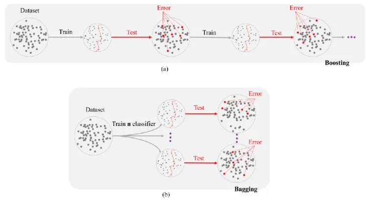
Fig. 5. The widely used ensemble learning methods: (a) Boosting and (b) Bagging.

methods, respectively. Furthermore, the one-shot multi-class classification uses fewer support vectors while, unlike the conventional one-against-all strategy, it guarantees to produce a complete confusion matrix [101]. SVM classifies high-dimensional big data into a limited number of support vectors, thus achieving the distinction between subgroups within a short period of time. However, the classification of big data is always computationally expensive. As such, hybrid methodologies of the SVM, e.g., Granular Support Vector Machine (GSVM), are introduced in different applications. GSVM is a novel machine learning model based on granular computing and statistical learning theory that addresses the inherently low-efficiency learning problem of the traditional SVM while obtaining satisfactory generalization performance [102].

SVMs are particularly attractive in the field of remote sensing owing to their ability to manage small training data sets effectively and often delivering higher classification accuracy compared to the conventional methods [97]–[99]. SVM is an efficient classifier in high-dimensional spaces, which is particularly applicable to remote sensing image analysis field where the dimensionality can be extremely large [100], [101]. In addition, the decision process of assigning new members only needs a subset of training data. As such, SVM is one of the most memory-efficient methods, since only this subset of training data needs to be stored in memory [108]. The ability to apply new kernels rather than linear boundaries also increases the flexibility of SVMs for the decision boundaries, leading to a greater classification performance. Despite these benefits, there are also some challenges, including the choice of a suitable kernel, optimum kernel parameters selection, and the relatively complex mathematics behind the SVM, especially from a non-expert

user point of view, that restricts the effective cross-disciplinary applications of SVMs [103].

B. Random Forest Classifier

RF is an ensemble learning approach, developed by [110], for solving classification and regression problems. Ensemble learning is a machine learning scheme to boost accuracy by integrating multiple models to solve the same problem. In particular, multiple classifiers participate in ensemble classification to obtain more accurate results compared to a single classifier. In other words, the integration of multiple classifiers decrease variance, especially in the case of unstable classifiers, and may produce more reliable results. Next, a voting scenario is designed to assign a label to unlabeled samples [11], [111], [112]. The commonly used voting approach is majority voting, which assigns the label with the maximum number of votes from various classifiers to each unlabeled sample [107]. The popularity of the majority voting method is due to its simplicity and effectiveness. More advanced voting approaches, such as the veto voting method, wherein one single classifier vetoes the choice of other classifiers, can be considered as an alternative for the majority voting method [108].

The widely used ensemble learning methods are boosting and bagging. Boosting is a process of building a sequence of models, where each model attempts to correct the error of the previous one in that sequence (see Fig. 5.a). AdaBoost was the first successful boosting approach, which was developed for binary classification cases [116]. However, the main problem of AdaBoost is model overfitting [111]. The Bootstrap Aggregating, known as Bagging, is another type of ensemble learning methods [117]. Bagging is designed to improve the

(6)

stability and accuracy of integrated models while reducing variance (see Fig. 5.b). As such, Bagging is recognized to be more robust against the overfitting problem compared to the boosting approach [110].

RF was the first successful bagging approach, which was developed based on the combination of Breiman’s bagging sampling approach, random decision forests, and the random selection of features independently introduced by [118]–[120]. RFs with significantly different tree structures and splitting variables encourage different instances of overfitting and outliers among the various ensemble tree models. Therefore, the final prediction voting mitigates the overfitting in case of the classification problem, while the averaging is the solution for the regression problems. Within the generation of these individual decision trees, each time the best split in the random sample of predictors is chosen as the split candidates from the full set of predictors. A fresh sample of predictors is taken at each split utilizing a user-specified number of predictors (Mtry). By expanding the random forest up to a user-specified number of trees (Ntree), RF generates high variance and low bias trees. Therefore, new sets of input (unlabeled) data are assessed against all decision trees that are generated in the ensemble, and each tree votes for a class’s membership. The membership with the majority votes will be the one that is eventually selected (see Fig. 6) [121], [122]. This process, hence, should obtain a global optimum [123]. To reach a global optimum, two-third of the samples, on average, are used to train the bagged trees, and the remaining samples, namely the out-of-bag (OOB) are employed to cross-validate the quality of the RF model independently. The OOB error is used to calculate the prediction error and then to evaluate Variable Importance Measures (VIMs) [117], [118].

Fig. 6. Random forest model.

Of particular RFs’ characteristic is variable importance measures (VIMs) [126]–[129]. Specifically, VIM allows a model to evaluate and rank predictor variables in terms of

relative significance [29], [51]. VIM calculates the correlation between high dimensional datasets on the basis of internal proximity matrix measurements [130] or identifying outliers in the training samples by exploratory examination of sample proximities through the use of variable importance metrics [49]. The two major variable importance metrics are: Mean Decrease in Gini (MDG) and Mean Decrease in Accuracy (MDA) [124]–[126]. MDG measures the mean decrease in node impurities as a result of splitting and computes the best split selection. MDG switches one of the random input variables while keeping the rest constant. It then measures the decrease in the accuracy, which has taken place by means of the OOB error estimation and Gini Index decrease. In a case where all predictors are continuous and mutually uncorrelated, Gini VIM is not supposed to be biased [29]. MDA, however, takes into account the difference between two different OOB errors, the one that resulted from a data set obtained by randomly permuting the predictor variable of interest and the one resulted from the original data set [110].

To run the RF model, two parameters have to be set: The number of trees (Ntree) and the number of randomly selected features (Mtry). RFs are reported to be less sensitive to the Ntree compared to Mtry [127]. Reducing Mtry parameter may result in faster computation, but reduces both the correlation between any two trees and the strength of every single tree in the forest and thus, has a complex inﬂuence on the classification accuracy [121]. Since the RF classifier is computationally efficient and does not overfit, Ntree can be as large as possible [135]. Several studies found 500 as an optimum number for the Ntree because the accuracy was not improved by using Ntrees higher than this number [123]. Another reason for this value being commonly used could be the fact that 500 is the default value in the software packages like R package; “randomForest” [136].

In contrast, the number of Mtry is an optimal value and depends on the data at hand. The Mtry parameter is recommended to be set to the square root of the number of input features in classification tasks and one-third of the number of input features for regression tasks [110]. Although methods based on bagging such as RF, unlike other methods based on boosting, are not sensitive to noise or overtraining [137], [138], the above-stated value for Mtry might be too small in the presence of a large number of noisy predictors, i.e., in the case of non-informative predictor variables, the small Mtry results in building inaccurate trees [29].

The RF classifier has become popular for classification, prediction, studying variable importance, variable selection, and outlier detection since its emergence in 2001 by [110]. They have been widely adopted and applied as a standard classifier to a variety of prediction and classification tasks, such as those in bioinformatics [139], computer vision [140], and remote sensing land cover classification [141]. RF has gained its popularity in land cover classification due to its clear and understandable decision-making process and excellent classification results [123], as well as easily implementation of RF in a parallel structure for geo-big data computing acceleration [142]. Other advantages of RF

(7)

Fig. 7. Article search query design.

classifier can be summarized as (1) handling thousands of input variables without variable deletion, (2) reducing the variance without increasing the bias of the predictions, (3) computing proximities between pairs of cases that can be used in locating outliers, (4) being robust to outliers and noise, (5) being computationally lighter compared to other tree ensemble methods, e.g., Boosting. As such, many research works have illustrated the great capability of the RS classifier for classification of Landsat archive, hyper and multi spectral image classification [143], and Digital Elevation Model (DEM) data [144]. Most RF research has demonstrated that RF has improved accuracy in comparison to other supervised learning methods and provide VIMs that is crucial for multi-source studies, where data dimensionality is considerably high [145].

III. METHODS

To prepare for this comprehensive review, a systematic literature search query was performed using the Scopus and the Web of Science, which are two big bibliographic databases

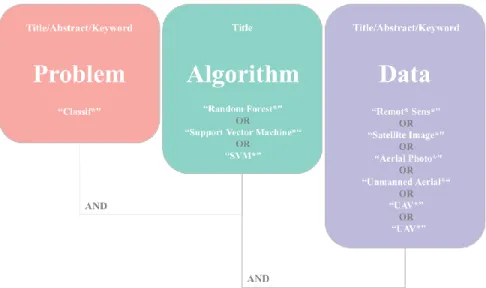
and cover scholarly literature from approximately any discipline. Notably, Preferred Reporting Items for Systematic Reviews and Meta-Analyses (PRISMA) were followed for study selection [146]. After numerous trials, three groups of keywords were considered to retrieve relevant literature in a combination on and up to October 28, 2019 (see Fig. 7). The keywords in the first and last columns were searched in the topic (title/abstract/keyword) to include papers that used data from the most common remote sensing platforms and addressed a classification problem. However, the keywords in the second column were exclusively searched in the title to narrow the search down. This resulted in obtaining studies that only employed SVM and RF algorithms in their analysis.

To identify significant research findings and to keep a manageable workload, only those studies that had been published in one of the well-known journals in the remote sensing community (see Table II) have been considered in this literature review.

TABLEII.REMOTE SENSING JOURNALS USED TO COLLECT RESEARCH STUDIES FOR THIS LITERATURE REVIEW.

Journal Publication Impact factor

(2019)

Remote Sensing of Environment Elsevier 8.218

ISPRS Journal of Photogrammetry and Remote Sensing Elsevier 6.942

Transaction on Geoscience and Remote Sensing IEEE 5.63

International Journal of Applied Earth Observation and Geoinformation Elsevier 4.846

Remote Sensing MDPI 4.118

GISience Remote Sensing Taylor & Francis 3.588

Journal of Selected Topics in Applied Earth Observations and Remote Sensing IEEE 3.392

Patterns Recognition Letters Elsevier 2.81

Canadian Journal of Remote Sensing Taylor & Francis 2.553

International Journal of Remote Sensing Taylor & Francis 2.493

Remote Sensing Letters Taylor & Francis 2.024

(8)

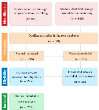
Fig. 8. PRISMA flowchart demonstrating the selection of studies.

Of the 471 initial number of studies, 251 were eligible

to be included in the meta-analysis with the following

attributes: title, publication year, first author, journal,

citation, application, sensor type, data type, classifier,

image processing unit, spatial resolution, spectral

resolution, number of classes, number of features,

optimization method, test/train portion, software/library,

single-date/multi-temporal, overall accuracy, as well as

some specific attributes for each classifier, such as

kernel types for SVM and number of trees for RF. A

summary of the literature search is demonstrated in Fig.

8.

IV. RESULTS AND DISCUSSION

A. General characteristics of studies

Following the in-depth review of 251 publications on supervised remotely-sensed image classification, relevant data were obtained using the methods described in Section III. The primary sources of information were articles published in scientific journals. In this section, we conduct analysis about the geographical distribution of the research papers and discuss the frequency of those papers based on RF and SVM considering time, journals, and application domains. This was followed by statistical analysis of remote sensing software packages used in the case studies, given RFs and SVMs. Further, we reported the result and discussed the finding of classification performance against essential features, i.e., data type, RS applications, spatial resolution, and finally, the number of extracted features.

(9)

Fig. 10. The usage rate of SVM and RF for remote sensing image classification in countries with more than three studies.

Fig. 11. Cumulative frequency of studies that used SVM or RF algorithms for remote sensing image classification.

Fig. 9 illustrates the geographical coverage of published papers based on the research institutions reported in the article on a global scale. More than three studies were published in 16 countries from six continents, including Asia 41%, Europe 32%, North America 18%, and the others 9%. As can be seen, most of the studies have been carried out in Asia and specifically in China by 71 studies; more than two times higher than the number of studies conducted in the following country (i.e., USA). The papers from China and the USA have been over 40% of the studies. This is maybe due to the extensive scientific studies conducted by the universities and institutions located in these countries, as well as the availability of the datasets. Fig. 10 also demonstrates the popularity of RF and SVM classifiers within these 16 countries. It is interesting that in the Netherlands and Canada, RF is frequently applied while in China and the USA, SVM attracts more scientists. It was only in Italy and Taiwan that all the studies used merely one of the classifiers (i.e., SVMs).

Fig. 11 represents the annual frequency of the publications

and the equivalent cumulative distribution for RF and SVM algorithms applied for remote sensing image classification. The resulting list of papers includes 251 studies published in 12 different peer-reviewed journals. Case studies were assembled from 2002 to 2019, a period of 17 years, wherein the first study using SVM dates back to 2002 [147] and 2005 for RFs [145]. The graph shows the significant difference between studies using SVM and RF over the time frame. Apart from a brief drop between 2010 and 2011, there was a moderate increase in case studies using SVM from 2002 to 2014. However, this slips back for four subsequent years, followed by significant growth in 2019. Studies using RFs, on the other hand, shows the steady increase in the given time-span, which resulted in an exponential distribution in the equivalent cumulative distribution function. The number of studies employed SVMs were always more than those that used RFs until 2016, wherein the number crossed over in favor of utilizing RFs. The sharp decrease in using both RF and SVM between 2014 and 2019 can be clearly explained by the advent of utilizing deep learning models in the RS community [148]. However, it seems that employing RF and SVM regained the researchers’ attention from 2018 onward. Overall, 170 (68%) and 105 (42%) studies used SVM and RF for their classification task, respectively. It is noteworthy to mention that some papers include the implementation of both methods. Besides, the graph illustrates that utilizing SVMs fluctuated more than RFs, and both classifiers keep almost steady growth, given the time period. More information on datasets will be given in the next section.

(10)

Fig. 12. The number of publications per journal; Remote Sensing of Environment (RSE), ISPRS Journal of Photogrammetry and Remote Sensing (ISPRS), Transaction on Geoscience and Remote Sensing (IEEE TGRS), International Journal of Applied Earth Observation and Geoinformation (JAG), Remote Sensing (RS MDPI), GIScience Remote Sensing (GIS & RS), Journal of Selected Topics in Applied Earth Observations and Remote Sensing (IEEE JSTARS), Patterns Recognition Letters (PRL), Canadian Journal of Remote Sensing (CJRS), International Journal of Remote Sensing (IJRS), Remote Sensing Letters (RSL), and Journal of Applied Remote Sensing (JARS).

Fig. 12 demonstrates the number of publications in each of these 12 peer-reviewed journals, as well as their contribution in using RF and SVM. Nearly one-fourth of the papers (24%) were published in Remote Sensing (RS MDPI) with the majority of the remaining published in the Institute of Electrical and Electronics Engineers (IEEE) hybrid journals (JSTARS, TGRS, and GRSL; 23%), International Journal of Remote Sensing (IJRS; 19%), Remote Sensing of Environment (RSE; 8%), and six other journals (26%). Although in most of the journals the number of SVM- and RF-related articles are high enough, three journals have published less than ten papers with RF or SVM classification implementations (i.e., GIS&RS, CJRS, and PRL).

The scheme for RS applications used for this study consisted of 8 broad Classification groupings referred to as classes distributed across the world (Fig. 13). The most frequently investigated application, representing 39% of studies, was related to land cover mapping, with other categorial applications including agriculture (15%), urban (11%), forest (10%), wetland (12%), disaster (3%) and soil (2%). The remaining applications comprising about 8% of the case studies mainly consist of mining area classification, water mapping, benthic habitat, rock types, and geology mapping.

Fig. 13. Number of Studies that used SVM or RF algorithms in different remote sensing applications.

B. Statistical and remote sensing software packages

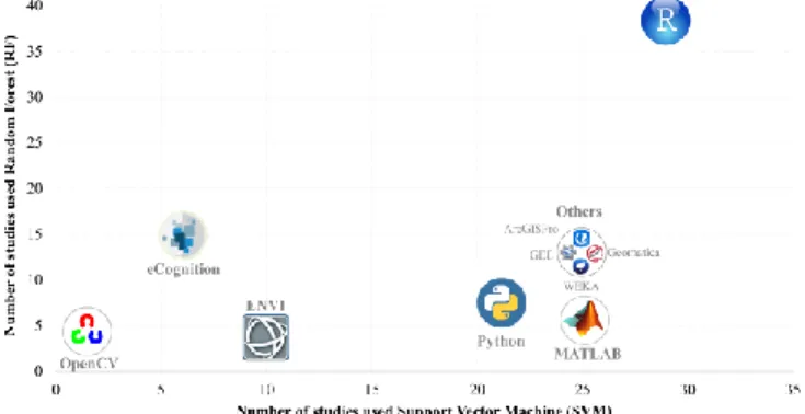
A comparison of the geospatial and image processing software and other statistical packages is depicted in Fig. 14. These software packages shown here were used for the implementation of both the SVM and RF methods in at least three journal papers. The software packages include eCognition (Trimble), ENVI (Harris Geospatial SolutionsInc.), ArcGIS (ESRI), Google Earth Engine, Geomatica (PCI Geomatics) as well as statistical and data analysis tools, which are Matlab (MathWorks), and open-source software tools such as R, Python, OpenCV, and Weka data mining software tool (developed by Machine Learning Group at the University of Waikato, New Zealand). A detailed search through the literature showed that the free statistical software tool R appears to be the most important and frequent source of SVM (25%) and RF (41%) implementation. R is a programming language and free software environment for statistical computing and graphics and widely used for data analysis and development of statistical software. Most of the implementations in R were carried out using the caret package [149], which provides a standard syntax to execute a variety of machine learning methods, and e1071 package [150], which is the first implementation of SVM method in R. The dominance of statistical and data analysis software especially R, Python (scikit-learn package), and Matlab is mainly because of the flexibility of these interfaces in dealing with extensive machine learning frameworks such as image preprocessing, feature selection and extraction, resampling methods, parameter tuning, training data balancing, and classification accuracy comparisons. In terms of the commercial software, for RF, eCognition is the most popular one, with about 17% of the case studies, while for the SVM classification method, ENVI is the most frequent software accounted for 9% of the studies.

Fig. 14. Software packages with tools/modules for the implementation of RF and SVM methods.

C. Classification performance and data type

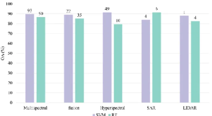
Considering the optimal configuration for the available datasets, Fig. 15 shows the average accuracies based on the type of remotely sensed data for both the SVM and RF methods. Multispectral remote sensing images remain undoubtedly the most frequently employed data source

(11)

amongst those utilized in both SVM and RF scenarios, with about 50% of the total papers mainly involving Landsat archives followed by MODIS imagery. On the other hand, the least data usage is related to LIDAR data, with less than 2% of the whole database. The percentages of the remaining types of remote sensing data for SVM are as follows: fusion (21%), hyperspectral (21%), SAR (4%), and LIDAR (1.6%). These percentages for RF classifiers are about 32%, 10%, 6%, and 4%, respectively. In working with the multispectral and hyperspectral datasets, SVM gets the most attention. However, when it comes to SAR, LIDAR, and fusion of different sensors, RF is the focal point. The mean classification accuracy of SVM remains higher than the RF method in all sensor types except in SAR image data. Although it does not mean that in those cases, the SVM method works better than RF, it gives a hint about the range of accuracies that might be reached when using the SVM or RF. Moreover, it can be observed that, except for hyperspectral data in case of using the RF method, the mean classification accuracies are generally more than 82%. For SVM, the mean classification accuracy of hyperspectral datasets remains the highest at 91.5%, followed by multispectral (89.7%), fusion (89.14%),

Fig. 15. Distribution of overall accuracies for different remotely sensed data (the numbers on top of the bars show the paper frequencies).

LIDAR (88.0%), and SAR (83.9%). This order for the RF method goes as SAR, multispectral, fusion, LIDAR, and hyperspectral with the mean overall accuracies of 91.60%, 86.74%, 85.12%, 82.55%, and 79.59%, respectively.

D. Classification performance and remote sensing applications

The number of articles focusing on different study targets (the number of studies is shown in the parenthesis) alongside the statistical analyses for each method is shown in Fig. 16. Other types of study targets, including soil, forest, water, mine, and cloud (comprising less than 10% of the total studies) were very few and are not shown here individually. The statistical analysis was conducted to assess OA (%) values that SVM and RF classifiers achieved for seven types of classification tasks. As shown in Fig. 16, most studies focused on LULC classification, crop classification, and urban studies with 50%, 14%, and 11% for SVM and 27%, 17%, and 14% for RF classifier. For LULC studies, the papers mostly adopted the publicly-available benchmark datasets, as the

main focus was on hyperspectral image classification. The most used datasets were from AVIRIS (Airborne Visible/Infrared Imaging Spectrometer) and ROSIS (Reflective Optics System Imaging Spectrometer) hyperspectral sensors. For crop classification, the mainly used data was AVIRIS, followed by MODIS imageries. While in urban studies, Worldview-2 and IKONOS satellite imageries were the most frequently employed data. On the other hand, other studies mainly focused on the non-public image dataset for the region under study based on the application. Therefore, there is a satisfying number of studies that have focused on the real-world remote sensing applications of both SVM and RF classifiers.

The assessment of classification accuracy regarding the types of study targets shows the maximum average accuracy in case of using RF for LULC with approximately 95.5% and change detection with about 93.5% for SVM classification. LULC, as a mostly used application in both SVM and RF scenarios, shows little variability for the RF classifier. It can be interpreted as the higher stability of the RF method than SVM in the case of classification. The same manner is going on in crop classification tasks (i.e., the higher average accuracy and little variability for RF compared to the SVM method). The minimum amounts of average accuracies are also related to disaster-related applications and crop classification tasks for RF and SVM, respectively.

Fig. 16. Overall accuracies distribution of (a) SVM and (b) RF classifiers in different applications.

E. Classification performance and spatial resolution

Fig. 17 shows the average obtained accuracy using RFs and SVMs based on the spatial resolution of the employed image

(12)

data and their equivalent number of published papers. The papers were categorized based on the spatial resolution into high (<10 m), medium (between 10 m and 100m), and low (>100 m). As seen, a relatively high number of papers (~49%) were dedicated to the image data with spatial resolution in the range of 10-100 m. Datasets with a spatial resolution of smaller than 10 m also contribute to the high number of papers with about 44% of the database. The remaining papers (~7% of the database) deployed the image data with a spatial resolution of more than 100 m. The image data with high, medium and low resolutions comprise 41%, 52%, and 7% of the studies for the SVM method and 52%, 44%, and 4% of the papers while using the RF method. Therefore, in the case of using high spatial resolution remote sensing imagery, RF remains the most employed method, while in the case of medium and low-resolution images, SVMs are the most commonly used method. A relatively robust trend is observed for the SVM method as the image data pixel size increases the average accuracy decreases. Such a trend can be observed for RF regarding that OA versus resolution is inconsistent among the three categories. Hence, in the case of the RF classifier, it is not possible to get a direct relationship between the classification accuracy and the resolution. However, in the High and Medium resolution scenarios, the SVM method shows the higher average OAs.

Fig. 17. Frequency and average accuracy of SVM and RF by the spatial resolution.

Fig. 18. Frequency and average accuracy of SVM and RF by the number of features.

F. Classification performance and the number of extracted features

Frequency and the average accuracies of SVMs and RFs versus the number of features are presented in Fig. 18. The

papers were split into three groups (<10, between 10 and 100, and >100) based on the employed number of features. As can be seen, the number of papers for the SVM method is relatively the same for the three groups. However, in the case of RF, the vast majority of published papers (over than 60% of the total papers) focused on using 10 to 100 features, whereas a smaller number of papers used the number of features less than 10 or higher than 100, i.e., 22% and 18%, respectively. The comparison of the average accuracies of RF and SVM methods shows that the SVM method is reported to have higher accuracy. However, because of the inconsistency of the average accuracies for both SVM and RF, it is not possible to predict a linear relationship between the number of features and acquired accuracies. For the SVM method, the highest reported average accuracy is when using the lowest (<10) and highest (>100) number of features, but RF shows the highest average accuracy while the number of features is between 10 and 100.

Fig. 19 displays the scatterplot of the sample data for pairwise comparison of RF and SVM classifiers. This figure illustrates the distribution of the overall accuracies and indicates the number of articles where one classifier works better than another. It can also help to interpret the magnitude of improvement for each sample article while considering the other classifier’s accuracy. To further inform the readers, we marked the cases with different ranges of the number of features by three shapes (square, circle, and diamond), and with different sizes. The bigger size indicates the lower spatial resolution, i.e., bigger pixel size.

Moreover, to analyze the sensitivity of the algorithms to the number of classes, a colormap was used in which the brighter (more brownish) color shows the lower number of classes, and as the number of classes increases, the color goes toward the dark colors. The primary conclusion that is observed from the scatter plot is that most of the points are near the line 1:1, which shows somewhat similar behavior of the classifiers. However, in general, there are 32 papers with the implementation of both classifiers, and in 19 cases (about 60%), RF outperforms SVM, and in 40% of the remaining papers, SVM reports the higher accuracy.

Fig. 19 organizes the results based on the feature input dimensionality in three general categories by using different shapes. When it comes to the number of features, one can clearly observe that there is only one circle below the line 1:1 while the others are at the above. This shows the better performance of the SVM when the input data contains many more features. This result is in accordance with those exploited from Fig. 18. Conversely, in the case of features between 10 and 100, there are over 63% of the squares under the identity line (7 squares out of 11), which shows the high capability of RF while working with this group of image data. Finally, considering features fewer than 10, 58% of the diamonds are under the identity line (11 out of 17) and 42% above the line. Considering the fraction of RF supremacy over SVM 60-40, it is hard to infer which method performs better.

To examine the spatial resolution, three shape sizes were used. It is hardly possible to notice a specific pattern with

(13)

Fig. 19. Comparison of the overall accuracy of SVM and RF classifiers by spatial resolution, number of features, and the number of classes in the under-study dataset.

respect to the pixel size of input data, but it is observed that most of the bigger shapes are under the one-to-one line. This represents the RF method offer consistently better results than SVM while dealing with images with bigger pixel size, which is in total accordance with Fig. 17. Looking at Fig. 19 and the distribution of points regarding the colors, the darker colors tend to offer more abundance under the identity line, while the points above the reference line are brighter. This can be proof of the efficiency of the SVM classifier to work with data with a lower number of classes. Statistically, 77% of the papers in which SVM shows higher accuracy include input data with the number of classes less than or equal to 6. The mean number of classes, in this case, is ~5.5, whereas the mean number of classes in which RF works better is 8.4.

V. RECOMMENDATIONS AND FUTURE PROSPECT Model selection can be used to determine a single best model, thus lending assistance to the one particular learner, or it can be used to make inferences based on weighted support from a complete set of competing models. After a better understanding of the trends, strengths, and limitations of RFs and SVMs in the current study, the possibility of integrating two or more algorithms to solve a problem should be more investigated where the goal should be to utilize the strengths of one method to complement the weaknesses of another. If we are only interested in the best possible classification accuracy, it might be difficult or impossible to find a single classifier that performs as well as an excellent ensemble of classifiers. Mechanisms that are used to build the ensemble of classifiers, including using different subsets of training data with a single learning method, using different training

parameters with a single training method, and using different learning methods, should be further investigated. In this sense, researchers may consider multiple variation of nearest neighbor techniques (e.g., K-NN) along with RF and SVM for both prediction and mapping.

Both SVM and RF are pixel-wise spectral classifiers. In other words, these classifiers do not consider the spatial dependencies of adjacent pixels (i.e., spatial and contextual information). The availability of remotely sensed images with the fine spatial resolution has revolutionized image classification techniques by taking advantage of both spectral and spatial information in a unified classification framework [144], [145]. Object-based and spectral-spatial image classification using SVM and RF are regarded as a vibrant field of research within the remote sensing community with lots of potential for further investigation.

The successful use of RF or SVM, coupled with a feature extraction approach to model a machine learning framework has been demonstrated intensively in the literature [153], [154]. The development of such machine learning techniques, which include a feature extraction approach followed by RF or SVM as the classifier, is indeed a vibrant research line, which deserves further investigation.

As discussed in this study, SVM and RF can appropriately handle the challenging cases of the high-dimensionality of the input data, the limited number of training samples, and data heterogeneity. These advantages make SVM and RF well-suited for multi-sensor data fusion to further improve the classification performance of a single sensor data source [155], [156]. Due to the recent and sharp increase in the availability of data captured by various sensors, future studies will investigate SVM and RF more for these essential

(14)

applications.

Several other ensemble machine learning toolboxes exist for different programming languages. The most widely used ones are scikit-learn [157] for Python, Weka [158] for Java, and mlj [159] for Julia. The most important toolboxes for R are mlr, caret [149], and tidy models [160]. Most recently, the mlr3 [161] package has become available for complex multi-stage experiments with advanced functionality that use a broad range of machine learning functionality. The authors of this study also suggest that researchers explore the diverse functionality of this package in their studies. We also would like to invite researchers to report their variable importance, class imbalance, class homogeneity, and sampling strategy and design in their studies. More importantly, to avoid spatial autocorrelation, if possible, samples for training should be selected randomly and spatially uncorrelated; purposeful samples should be avoided. For benchmark datasets, this study recommends researchers to use the standard sets of training and test samples already separated by the corresponding data provider. In this way, the classification performance of different approaches becomes comparable. To increase the fairness of the evaluation, remote sensing societies have been developing evaluation leaderboards where researchers can upload their classification maps and obtain classification accuracies on (usually) nondisclosed test data. One example of those evaluation websites is the IEEE Geoscience and Remote Sensing Society Data and Algorithm Standard Evaluation website (http://dase.grss-ieee.org/).

VI. CONCLUSIONS

The development of remote sensing technology alongside with introducing new advanced classification algorithms have attracted the attention of researchers from different disciplines to utilize these potential data and tools for thematic applications. The choice of the most appropriate image classification algorithm is one of the hot topics in many research fields that deploy images of a vast range of spatial and spectral resolutions taken by different platforms while including many limitations and priorities. RF and SVM, as well-known and top-ranked machine learning algorithms, have gained the researchers’ and analysts’ attention in the field of data science and machine learning. Since there is ongoing employment of these methods in different disciplines, the common question is which method is highlighted based on the task properties. This paper focused on a meta-analysis of comparison of peer-reviewed studies on RF and SVM classifiers. Our research aimed to statistically quantify the characteristics of these methods in terms of frequency and accuracy. The meta-analysis was conducted to serve as a descriptive and quantitative method of comparison using a database containing 251 eligible papers in which 42% and 68% of the database include RF and SVM implementation, respectively. The surveying carried out in the database showed the following:

-The higher number of studies focusing on the SVM classifier is mainly due to the fact that it was introduced years before RF to the remote sensing community. As can be

concluded from the articles database, in the past three years, implementing the RF exceeded the SVM method. Nevertheless, in general, there is still an ongoing interest in using RF and SVM as standard classifiers in various applications.

-The survey in the database revealed a moderate increase in using RF and SVM worldwide in an extensive range of applications such as urban studies, crop mapping, and particularly LULC applications, which got the highest average accuracy among all the applications. Although the assessment of the classification accuracies based on the application showed rather high variations for both RF and SVM, the results can be used for method selection concerning the application. For instance, the relatively high average accuracy and the little variance of the RF method for LULC applications can be interpreted as the superiority of RFs over SVMs in this field.

-Medium and high spatial resolution images are the most used imageries for SVM and RF, respectively. It is hardly possible to notice a specific pattern concerning the spatial resolution of the input data. In the case of low spatial resolution images, the RF method offers consistently better results than SVM, although the number of papers using SVM for low spatial resolution image classification exceeded the RF method.

-There is not a strong correlation between the acquired accuracies and the number of features for both the SVM and RF methods. However, a comparison of the average accuracies of RF and SVM methods suggests the superiority of the SVM method while classifying data containing many more features.

Contrary to the dominant utilization of SVM for the classification of hyperspectral and multispectral images, RF gets the attention while working with the fused datasets. For SAR and LIDAR datasets, the RF was also used more than the SVM method. However, its popularity cannot be concluded because of the low available number of published papers.

ACKNOWLEDGMENT

This work has received funding from the European Union's the Innovation and Networks Executive Agency (INEA) under Grant Agreement Connecting Europe Facility (CEF) Telecom project 2018-EU-IA-0095.

REFERENCES

[1] C. Toth and G. Jóźków, “Remote sensing platforms and sensors: A survey,” ISPRS J. Photogramm. Remote Sens., vol. 115, pp. 22–36, 2016.

[2] M. Wieland, W. Liu, and F. Yamazaki, “Learning Change from Synthetic Aperture Radar Images: Performance Evaluation of a Support Vector Machine to Detect Earthquake and Tsunami-Induced Changes,” Remote Sens., vol. 8, no. 10, p. 792, Sep. 2016, doi: 10.3390/rs8100792. [3] K. Wessels et al., “Rapid Land Cover Map Updates Using

Change Detection and Robust Random Forest Classifiers,”

Remote Sens., vol. 8, no. 11, p. 888, Oct. 2016, doi:

10.3390/rs8110888.

[4] F. Traoré et al., “Using Multi-Temporal Landsat Images and Support Vector Machine to Assess the Changes in