Mantle dynamics and geoid Green functions

HAL Id: hal-02046761

https://hal.archives-ouvertes.fr/hal-02046761

Submitted on 3 Feb 2021

HAL is a multi-disciplinary open access

archive for the deposit and dissemination of

sci-entific research documents, whether they are

pub-lished or not. The documents may come from

teaching and research institutions in France or

abroad, or from public or private research centers.

L’archive ouverte pluridisciplinaire HAL, est

destinée au dépôt et à la diffusion de documents

scientifiques de niveau recherche, publiés ou non,

émanant des établissements d’enseignement et de

recherche français ou étrangers, des laboratoires

publics ou privés.

Mantle dynamics and geoid Green functions

V. Corrieu, C. Thoraval, Y. Ricard

To cite this version:

V. Corrieu, C. Thoraval, Y. Ricard. Mantle dynamics and geoid Green functions. Geophysical

Journal International, Oxford University Press (OUP), 1995, 120 (2), pp.516-523.

�10.1111/j.1365-246X.1995.tb01835.x�. �hal-02046761�

R E S E A R C H NOTE

Mantle dynamics and geoid Green functions

Valerie Corrieu, Catherine Thorava12 and

Y

anick R i ~ a r d ' ? ~

'

Dipartement TAO, Ecole Normale Supe'rieure, 24 rue Lhomond, 75231 Paris Cedex 05, France

'

GRGS-CNES. 18 avenue Edouard Belin, 310.55 Toulouse Cedex, France

'

E N S , Diparlemenr de Geologie, 46 alle'e d'lralie, 69364 Lyon cedex, France Accepted 1994 August 9. Received 1994 August 9; in original form 1994 May 13

S U M M A R Y

We compute Green functions relating mantle mass heterogeneities to geoid undulations using both incompressible and radially compressible mantle rheologies. Our results differ from those previously published by Forte & Peltier (1991) and Thoraval, Machete1 & Cazenave (1994). This is due to two factors. Instead of taking gravity as constant throughout the mantle, we compute it self-consistently with the radial density profile. Secondly, we show that in the mathematical formulation

of

the compressible case, stresses are not continuous through a density jump. We then point out that the presence

of

a surface ocean has

no

additional effect

on

the geoid signal associated with internal mantle mass anomalies. We apply this formalism to a geodynamic model

of

mantle density variations and show that an excellent fit to the observed geoid can be obtained.

Key words:

geoid, Green's functions, mantle.

INTRODUCTION

In the last 10 years, geodynamicists have studied mantle dynamics using two complementary approaches. On the one hand, convection models have been developed. These models solve both thermal and mechanical equations. Their goal is to explain the structure and evolution of the mantle, but their results are not directly compared with the present-day state of the Earth. On the other hand, pure circulation models make the introduction of observations (gravity, plate motions, seismic velocity heterogeneities) much easier, but they usually d o not address the temporal evolution of mantle anomalies. .

The second approach generally involves the use of Green functions G ' ( r ) that relate a mass anomaly of degree 1 located at a given depth r to its physical consequences (i.e. induced gravity, topography, or surface velocity divergence). For example, the geoid coefficient NIm of degree I and order

m can be computed from the depth-dependent mass anomalies having the same harmonic degree and order,

SPlm, by:

In this equation, y is the gravitation constant, g, is the surface gravity, and the mantle extends from the core-mantle boundary CMB at radius c to the surface at radius a. The normalizing factor before the integral is such that G'(r) = 1 for a surface mass 6 ( r

-

n ) on top of a rigid Earth (6 is the Dirac function).

This formalism is only valid if the mantle is spherically symmetrical and has a Newtonian viscosity which depends only upon depth. A first generation of models (Ricard, Fleitout & Froidevaux 1984; Richards & Hager 1984)

516

assumes an incompressible mantle. In that case, any density jump in the model corresponds to a non-adiabatic barrier to radial fiow. A second generation of models introduces compressibility both in the Cartesian case (Hong & Yuen 1990) and in the spherical case (Dehant & Wahr 1991; Forte

& Peltier 1991; Thoraval et al. 1994). The differences

between the Green functions computed using compressible or incompressible models are not striking, but they can reach about 10 per cent. However, it appears that some mismodelling is present in previous computations in spherical geometry. Here we address this point.

CONSTITUTIVE EQUATIONS

The mantle flow obeys the following equations describing the conservation of mass and momentum, the gravitation (Poisson's equation), and the compressible rheology:

aP pVv+-vVr=O, ar %r

+

p v u

+

6pg = 0, ₍₃₎

v2u

= -4nysp, u = T(T,

+

Tvt -

$SjjTV) - p l ,

where I is the identity matrix and 6 , is the Kronecker symbol. In these equations, some variables are only depth dependent: the viscosity q, the reference density p, and the radial gravity g. The other variables are 3-D fields: the velocity vector v, with radial component u,, the stress tensor

u, the perturbation of the gravity potential U, the

non-hydrostatic pressure p and the mass anomaly field 6p.

We make several approximations in writing these

Mantle dynamics

517

A =

equations. In the continuity equation (2) we ignore the density time derivative, and we neglect lateral density variations. We also neglect the second-order term GpVU in Compressibility has various effects. First, the continuity equation (2) shows that the velocity of a down-going flow decreases as the density of the mantle increases with depth. Secondly, the self-gravitation term pVU in eq. (3) takes into account the radial density variation. Only compressible models can be used to model seismologically inferred radial density profile. Third, the rheological behaviour (eq. 5) is also changed.

As a consequence of compressibility, the pressure perturbation induces density variations in the whole mantle. One cannot distinguish between the 'direct' mass anomalies, for example, related to thermal variations, and the mass anomalies induced by compressibility. Thus, in eqs (3) and

(4), 6p represents any lateral variation of density, whatever its cause.

To solve eqs (2)-(S), the following change of variables is performed (Hager & O'Connell 1979).

eq. (3). v, = u , Y , v, = u* Yo, v* = UZ Y*, (6) 770 77 -1 1 0 - 0 0 4 ( 3 + k ) - 77 -6L- 77 1 L 0 - - P , 770 770 Po 770 r urr = - ug Y, 770 770 U = - u U , Y , - = 7 u s Y , Po' ar Po' a,, =

2

u4 Y,, r

where u, are only functions of the radius r and where

a

'-ae

Y - - Y (7) and y Y.

In this formalism, p0 and qo are constant reference values. The change of variables used in eqs ( 6 ) and (7) is not the

most general. It neglects the toroidal field which cannot be excited in a Newtonian mantle with spherically symmetrical rheology (e.g. Hager & O'Connell 1979).

Introducing these new variables into eqs (2)-(5) and using the orthogonality properties of spherical harmonics, the following differential system of the vector P = ui is found

i

a

.P - sin

(e) a+

d P dr r - = AP

+

a, where,

(

- 2 - k L 0 0 0 0 1 (9) Po -2(3+k)- 77 2(2L-1)-

v

-1 -2 - - 770 770 0 0 L 0 O 0

' 1

0 0

with L = f(f

+

I), and

mr2,

0, 0, -

4nyp0Gpr3i

770

a =

o,o,

~ 770

The only difference between these equations and those found in the incompressible case (e.g. Hager & O'Connell 1981) is the compressibility factor k = d In p / d In r and the

fact that the density p can now be a depth-dependent function.

This system looks somewhat different from what has been published. However, it is exactly equivalent to the equations of Forte & Peltier (1991) who use a more elegant set of basis functions: the generalized spherical harmonics. It is also equivalent to the results of Thoraval et al. (1994), who obtain different diagonal terms but use pu, instead of u i as variables.

From this point on, the treatment of the equations differs from previous work. Forte & Peltier (1991) and Thoraval ef al. (1994) assume that at a density discontinuity, the

horizontal velocity, the vertical velocity times the density, the radial stress and the horizontal shear stresses are continuous. Using the superscripts - and

+

for the layers

below and above the discontinuity, they write:

(12)

p u , = p - u ; , u: = u;,

u; = u;, u,' =

uq.

(13) + +

However, these conditions are inconsistent with eqs (9) and (10). To show this, we introduce a thin shell of uniform thickness E between the layers - and

+.

The com-

pressibility factor of this layer k = In ( p + / p - ) / l n ( r + / r - ) being very large as r - is close to r + . When E

tends to zero, the changes of the variables through this layer should be equivalent to those given by eqs (12) and (13). As the system (9) is still valid when the viscosity varies radially,

we assume that the viscosity in the thin layer varies linearly between the viscosities 17- and

vf.

Integrating the system of equations over E, we derive:

u: =

[

)m+ exp ( l A / r d r ) ] u ; . (14) The only finite terms to consider in eq. (14) and those that include k in the matrix A since h-+,+ [ k In ( r + / r - ) ]

remains finite and equal to In ( p + / p - ) . After some algebra, eq. (14) can be rewritten in the following form:

(15) + + p u1 = p - u ; , u; = u;, 77+ + 77- u; = u; - 2-(u; - u ; ) , 770

u4' =

uq

+=(u: - u;).

770

This shows that through a density jump related to compressibility, the stresses in, our formulation cannot be treated as continuous and that the discontinuity is proportional to the effective jump in the vertical velocity. Of course, in the case of no density jump, or if the boundary is a 'chemical boundary' which the flow cannot cross

(u: = u ; =O), u l is continuous and eqs (15)-(17) reduce to eqs (12) and (13). One should also note that it is not possible to put a discfete mass anomaly at the boundary because the value of 6 p (eq. 11) is not determined.

Why is this stress discontinuity? The standard physical trick used to account for an interface is to apply the mechanical equations to a rectangular pill-box including the interface. As an example, in the 2-D Cartesian case one can write the horizontal conservation of momentum

aa,,

do;,

ax +-=O. az

After a vertical integration, the vertical variation of the horizontal shear uTz -

upz

appears to be related to the integral of the horizontal variations of the horizontal normal stress through the vertical side of the box,

ax d z ) .

In an incompressible flow, the horizontal stress is finite, so

when the vertical size of the box tends to zero, uTz = u,.

The problem in a compressible fluid is, however, different; when the thickness of the layer in which the density increases tends to zero, the horizontal stress tends to infinity. In this case, the integral of the horizontal stress through the box side remains finite when the box size tends to zero. Thus, the shear stress is not continuous. For the Earth, due to sphericity, the vertical stress is also discontinuous. It should be noted that these discontinuities in density and stress are artefacts of the mathematical formulation, in which all calculations are done at radial reference boundaries. Thus, the discontinuities result from standard Taylor series approximations, and they should not be taken too literally.

Another difference between our calculations and those of Forte & Peltier (1991) and Thoraval et al. (1994) is that we

use a depth-dependent gravity profile corresponding to the chosen depth-dependent density profile, instead of constant gravity. According to PREM the Earth’s gravitational acceleration vanes from 9.8msP2 at the surface to 10.7 ms-’ at the CMB. This variation of 10 per cent is of the same order as the differences between the compressible and incompressible Green functions. It should thus be taken into account.

B O U N D A R Y CONDITIONS

To compute Green functions one also needs to state the boundary conditions. At the interface between solid Earth and air or water, or at the CMB, free slip conditions are chosen: the vertical velocity and the shear stresses are equal to zero. The assumption of zero vertical velocity at chemical interfaces implies that we deal with phenomena that occur with time constants much larger than those of postglacial rebound. The vertical stress jump a,: - a, at any density interface not related to compressibility is proportional to the local dynamic topography h. Above sea-level, the vertical stress u,: is zero. Below the sea-floor, the radial normal stress is related to the pressure caused by the gravity

potential undulations, since the sea surface follows the equipotential, and, in addition, to the deflection ha at the surface of the solid Earth. Thus below the surface a :

where a,,(a) is computed on the mantle side and where pw

is the water density. Similarly at the CMB, on the mantle

side

U A C ) = - p c U ( c ) - [ P A C ) - Pcl&h,, ₍₁₉₎

where p, is the density on the core side and h, is the CMB topography.

The gravity potential U at any depth r can be expressed as the sum of two potentials: the contribution of the masses above r, U + and the contribution of the masses below r,

U-. According to Poisson equation, U’ varies as r‘ and U - as r-(’+’). Thus, we can write either

au

1 + 1 2 1 + l - U + - U + , ar r r or

au

I 21+1 -

u--

U - ar r r

The potential anomaly U, at a depth r, due to the mass anomaly Sm, located at the same depth is:

We now apply eqs (20) and (21) at the surface and at the CMB, both on the mantle side. Below the surface, the potential U’ is due to both deformations of the sea surface and of the solid Earth surface. As the ocean surface follows the geoid, its topography is

U -

g ‘

Therefore, U + is given by:

where E is the ocean depth. Since E is small in comparison

with the Earths radius, we can write from eqs (18), (20), and (23):

au

1 + 1 4zy

ar - a

u

- -

ga urr.

In this equation, we implicitly identify potential values both at the surface and at the bottom of the sea. To do that, we neglect the term 4 z y p w l ~ / g a in front of 1

+

1. The ratio between these two terms is indeed smaller than loP4.

Above the CMB, U - is due only to the core topography. Hence, readily, we have:

The effect of compressibility in the core has been discussed by Ricard et al. (1984). Assuming that k varies as r an analytical correction can be added to eq. (23) but this correction is negligible at all degrees except degree 2 where it can reach a few per cent. This has been corroborated by Thoraval et al. (1994) who use the real depth-dependent compressibility of the core.

To obtain the Green functions, we must compute the vector (ur, v,, rrr,

rrO,

U , aUlar) as a function of depth. The solution can be found since six boundary conditions are

known: zero vertical velocities and shear stresses at the surface and CMB, plus eqs (24) and (25). The presence of

Mantle

dynamics

519

the ocean does not appear in these boundary conditions nor in the differential system (9). Therefore we conclude that the surface ocean has no significant effects on the computed velocities, stresses and geoid. The treatment of the geoid green functions was done correctly by both Ricard et a/.

(1984) and Richards & Hager (1984). Of course, the solid Earth topography induced by a given radial stress, eq. (18), is modified by the presence of the water. The sea warping effect discussed by Forte & Peltier (1991) and Thoraval et a/.

(1994) results from confusing two models: one in which the sea-water surface follows the geoid, and the other in which the sea-water surface unrealistically remains spherical.

The effect of crust is also for the same reason negligible in computing the geoid at long wavelength. In eq. (18), its presence would result in a new term related to the Moho topography. However, the sum of the different contributions of the surface masses to the potential (sea surface, surface topography, moho topography) would lead to an effect almost equal to that obtained in a model without crust. This approximation is again very small, of order

RESULTS

Figures l(a) and l(b) depict the geoid Green functions for compressible and incompressible mantle models. In (a), the mantle viscosity is uniform. In (b), the upper mantle is overlain by a lithosphere 10 times more viscous and lies over a lower mantle 50 times more viscous. The thick lines describe the results obtained using the density profile of PREM (Dziewonski & Anderson 1981), the dashed lines are for a uniform mantle of density 4450kgm-3. The core density at the CMB needed in eq. (23) is 9903 kg m-3. We choose a CMB gravity g, (eq. 23) of 10.68 m s-* according to PREM. The gravity profile in the mantle is consistent with the radial density profile and leads to the usual surface gravity of 9.8 m s-’. The differences between the compres- sible and incompressible cases amount to about 10 per cent but can be higher at some depths. This order of magnitude is in agreement with the results of Forte & Peltier (1991). However, the difference between their Green functions and ours (for both the compressible and incompressible cases) also amounts to or exceeds 10 per cent. We assume that this is due to their choice of constant gravity and to incorrect matching conditions at internal boundaries (eq. 13 instead of eqs 16 and 17). For the incompressible case, our results agree perfectly with those obtained by Richards & Hager (1984). A summary of the different parameters used is given in Table 1.

Organized the same way as Fig. 1, Fig. 2 shows the effect of the discontinuity of stresses at internal density jumps (670, 400 and 220km depth). The thick lines are geoid kernels for models including the discontinuity (eqs 15-17), the dashed lines are computed using eqs (12) and (13) that do not take into account the stress discontinuity. The difference between the two sets of functions is somewhat comparable with the difference between the compressible and the incompressible case.

Using mass anomalies deduced from mantle tomography or from slab reconstructions, the geoid Green functions have been used to infer the radial mechanical properties of the Earth. For example, Ricard et a/. (1993) have shown that a mass distribution deduced from Cenozoic and Mesozoic plate reconstructions is well correlated with seismic

E Y

G

n Q Q) E Y 5 n a Q)

Geoid Amplitude

r

1

380

-

.----..

₁

_:I:,’

I-.-...- 2880

2380

-0.4

i

-0.3 -0.2

-0.1

0.0

0.1 380 880 1380 1 a80 2380 2880

-0.1

0.0

0.1 0.2

0.3

0.4

Figure 1. Geoid Green functions for degrees 1 = 2, 5, 10. In the top panel (a) the mantle viscosity is uniform. In the bottom panel (b), a lOOkm depth lithosphere overlies a 10 times less viscous upper mantle. At 670 km, the viscosity jumps by a factor 50. The surface radius is 6368 km, the CMB radius is 3480 km. The compressible Green functions are depicted with a thick line, the incompressible results with a dashed line. The difference between the compressible and incompressible cases is of order 10 per cent and does not decrease when I increases.

observations and explains as much as 84 per cent of the total geoid variance. This mantle mass anomaly model simply assumes that slabs are sinking vertically through the mantle. The vertical velocity of the slabs is equal in the upper mantle to the convergence rate at the palaeo-subduction zones, and is reduced by a factor 4.4 at 670 km depth. This value is chosen to give the best possible correlation with the global seismic tomography model of Su & Dziewonski (1991). The mass density of each slab is simply proportional to the square root of its age at subduction.

The best fit between the observed geoid and that computed with a simple Earth model consisting of three incompressible layers (lithosphere, upper mantle and lower mantle) is obtained when these layers have relative viscosities of about

v,itho

= 10,

vUpprr

= 1,

vIower

= 40 (Ricard et al. 1993). Using the same mass distribution, and the same simple three-layer model, we compute the new geoid with compressible Green functions. Fig. 3 depicts the variance reduction achieved by our model as a function of

Density profile

Table 1. Density and gravity parameters used in both incompressible and compres-

sible mantle models.

I

uniform

I

PREM

Core density at the CMB Gravitv at t h e CMR

11

4450 kg/m3

I

including its discontinuities

/I

II

_I

and discretized over 25 layers

9903 kg/m3

i n f i ~ ,,,iFZ

J -. ._ --."" " ' I "

Mantle gravity profile Computed from CMB gravity

and Mantle density profile _-

Geoid Amplitude

380 880 E Y 1380

G

_Q. a 0 1880 2380 2880 -0.4 -0.3 -0.2 -0.1 0.0 0.1 E Y

s

0"

Q. -0.1

0.0

0.1

0.2

0.3

0.4

Figure 2. Geoid Green functions for degrees 1 = 2, 5, 10. In the top panel (a) the mantle viscosity is uniform. In the bottom panel (b), a 100km depth lithosphere overlies a 10 times less viscous upper mantle. At 670 km, the viscosity jumps by a factor 50. The mantle is compressible. The Green functions taking into account the discontinuity of stresses at internal density jumps are depicted with a thick line, the results neglecting this discontinuity, with a dashed line. The differences between the two cases are not negligible.

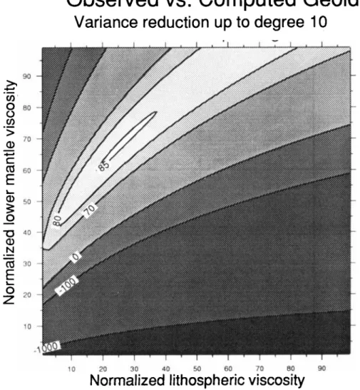
the lithospheric and lower mantle viscosities. The upper mantle has a reference viscosity value of 1. The best variance reduction is obtained for qlitho = 25, qlower = 67 and amounts to 85 per cent when all degrees and orders

from 2 to 10 are taken into account. This variance reduction

is of the same order as that obtained using incompressible Green functions, but with somewhat larger viscosity contrasts. The fact that higher viscosity contrasts are required by compressible models to fit the geoid agrees with the findings of Thoraval et al. (1994) but is in disagreement

with Forte & Peltier (1991). Satisfactory variance reductions are obtained for a viscosity jump at 670 km depth of at least a factor of 30. Larger viscosity contrasts at depth are also acceptable if the lithosphere is stiffer.

The best predicted geoid is shown in Fig. 4 (bottom map). Its agreement with the observed geoid (top map) is striking, considering the simplicity of the dynamic model. Although constructed with slightly different viscosity parameters, it closely resembles that published in Ricard et al. (1993, Fig. 9).

CONCLUSIONS

We hope to have clarified some problems in the computation of compressible geoid Green functions. Correct modelling must take into account the depth dependence of gravity and the effective discontinuity of stresses at internal adiabatic density jumps. However, the effects of compres- sibility on the geoid modelling are minor. They modify the kernels by an amount comparable with that caused by other approximations (e.g. constant mantle gravity) or mismodell- ing (continuity of stresses at density jump). At long wavelengths, thin surface layers such as the crust or the ocean are negligible in computing the geoid Green functions. The inferred mantle viscosity profile obtained by modelling the geoid is only slightly modified by compressible Green functions. Indeed, using a geodynamic model of

mantle density heterogeneity, the same variance reduction is obtained with compressible or incompressible rheologies, but with a somewhat larger increase of viscosity with depth for the compressible case.

ACKNOWLEDGMENTS

This work benefited from discussions with M. A. Richards (University of California at Berkeley) and benchmark tests using his incompressible kernels. Some benchmark with compressible kernels have also been performed with P. Defraigne (Observatoire Royal de Belgique) and L. Panasyuk (MIT). The study has been partly supported by the INSU Dynamique et Bilan de la Terre program;

Dynamique Globale, Contribution 707.

Mantle dynamics

521

Observed vs. Computed Geoid

Variance reduction up to dearee

10

L,

P

0

-

90 80 70 60 50 40 30 20 10 10 20 30 40 50 60 70 80 90

Normalized lithospheric viscosity

Figure 3. Contour plot of variance reduction of the observed geoid obtained from a dynamic model using compressible Green functions. The

variance is plotted as a function of lithospheric viscosity/upper mantle viscosity and of lower mantle viscosity/upper mantle viscosity. The best variance reduction obtained is 85 per cent. A satisfactory variance reduction is achieved if the lower mantle is at least 30 times more viscous than the upper mantle.

Figure 4. Observed (top) and best-fitting geoid (bottom) up to degree and order 15. The best-fitting geoid is obtained with a three-layer viscosity profile (25 in the lithosphere, 67 in the lower mantle, the upper mantle viscosity being taken as 1). The mantle density variations have been deduced from a model of Cenozoic and Mesozoic plate motion (Ricard et al. 1993). The contour interval is 20m.

Mantle dynamics 523 R E F E R E N C E S

Dehant, V. & Wahr, J.M., 1991. The response of a compressible, non-homogeneous Earth to internal loading: theory, J . Geomagn. Geoelect., 43, 157-178.

Dziewonski, A.M. & Anderson, D.L., 1981. Preliminary reference Earth model, Phys. Earth planet. Inter., 25, 297-356.

Forte, A.M. & Peltier, W.R., 1991. Viscous flow models of global geophysical observables, 1, Forward problems, J. geophys. Res., Hager. B.H. & O’Connell, R.J., 1979. Kinematic models of

large-scale flow in the Earth’s mantle, J. geophys. Res., 84, Hager, B.H. & O’Connell, R.J., 1981. A simple global model of plate dynamics and mantle convection, J . geophys. Res., 86, %,20 131-20 159.

1031 -1048.

4843-4867.

Hong, H. & Yuen, D.A., 1990. Dynamical effects from equation of state on topographies and geoid anomalies due to internal loading, J . geophys. R e x , 95, 19933-19 948.

Ricard, Y., Fleitout, L. & Froidevaux, C., 1984. Geoid heights and lithospheric stresses for a dynamic Earth, Ann. Geophys., 2, 267-286.

Ricard, Y., Richards, M.A., Lithgow-Bertelloni, C. & Le Stunff, Y.,

1993. A geodynamic model of mantle density heterogeneity, J. geophys. Res., 98,21 895-21 909.

Richards, M.A. & Hager, B.H., 1984. Geoid anomalies in a dynamic Earth, J . geophys. Res., 89, 5987-6002.

Su, W.J. & Dziewonski, A.M., 1991. Predominance of long wavelength heterogeneity in the mantle, Nature, 352, 121-126. Thoraval, C., Machetel, P. & Cazenave, A., 1994. Influence of mantle compressibility and ocean warping on dynamical models