Symbol and Spatial Relation Knowledge Extraction Applied to On-Line Handwritten Scripts

(1)

HAL Id: tel-00785984

https://tel.archives-ouvertes.fr/tel-00785984

Submitted on 7 Feb 2013

HAL is a multi-disciplinary open access

archive for the deposit and dissemination of sci-entific research documents, whether they are pub-lished or not. The documents may come from teaching and research institutions in France or abroad, or from public or private research centers.

L’archive ouverte pluridisciplinaire HAL, est destinée au dépôt et à la diffusion de documents scientifiques de niveau recherche, publiés ou non, émanant des établissements d’enseignement et de recherche français ou étrangers, des laboratoires publics ou privés.

Applied to On-Line Handwritten Scripts

Jinpeng Li

To cite this version:

Jinpeng Li. Symbol and Spatial Relation Knowledge Extraction Applied to On-Line Handwritten Scripts. Automatic Control Engineering. Université de Nantes Angers Le Mans, 2012. English. �tel-00785984�

(2)

Thèse de Doctorat

Jinpeng Li

Mémoire présenté en vue de l’obtention du

grade de Docteur de l’Université de Nantes

sous le label de l’Université de Nantes Angers Le Mans Discipline : Informatique

Spécialité : Automatique et Informatique Appliquée

Laboratoire : Institut de Recherche en Communications et Cybernétique de Nantes (IRCCyN) Soutenue prévue le 23 Octobre 2012

École doctorale : 503 (STIM) Thèse n° :

Extraction de connaissances symboliques et

relationnelles appliquée aux tracés manuscrits

structurés en-ligne

Symbol and Spatial Relation Knowledge Extraction Applied to On-Line Handwritten Scripts

JURY

Rapporteurs : M. Eric ANQUETIL, Professeur des Universités, Institut National des Sciences Appliquées de Rennes

M. Salvatore-Antoine TABBONE, Professeur des Universités, Université de Lorraine

Examinateur : M. Jean-Marc OGIER, Professeur des Universités, Université de La Rochelle

Directeur de thèse : M. Christian VIARD-GAUDIN, Professeur des Universités, Université de Nantes

(3)

(4)

Acknowledgements

The subject of this thesis was originally proposed by my supervisors, Prof. C. Viard-Gaudin and Doct. H. Mouchère. Therefore, specially thank you for my su-pervisors’ thesis, suggestions, correcting of all my papers, funding of “Allocation de Recherche du Ministère” and “Projet DEPART”, etc. It is a really new and challenging subject, which has been largely unexplored until now. Knowledge ex-traction is not only for prediction, but also for human understanding. In addition, thanks to many chances of international conference participations (CIFED2010, IC-DAR2011, KDIR2011, DRR2012, CIFED2012, ICFHR2012), I earned experiences to talk to people from different countries and known what the other people are do-ing. Thanks to an opportunity to organize a small seminar “séminaire au vert” with Sofiane and help a seminar “franco-chinois” in Polytech’Nantes. Thanks also to academic suggestions from Guoxian, Montaser, Sofiane, and Zhaoxin. Further-more, thank you for all the people from the team IVC of IRCCyN, e.g. for small delicious drinkings (“pot” in French) from different countries. I am grateful for ju-ries and examinator, Prof. Anquetil, Prof. Tabbone and Prof. Ogier, to take the time to review my thesis.

Concerning living in Nantes, thank you for my friends who helped me: Jiefu, Hongkun, Junle, LiJing, Jiazi, Dingbo, Zhujie, Baobao, Chuanlin, Fengjie, Hugo, Baptiste, Zhangyu, Wenzi, He HongYang, Junbin, Zhangyang, Biyi, Shuangjie, Zhaoxin, Tan Jiajie, Cédric, Dan, Zeeshan, Pierre, Emilie, and so on.

At the end, really thank you for my wife Huanru coming at Nantes for the end of my thesis, and allowing me that always focus on my interesting works.

(5)

(6)

1

Introduction

Since paper and pen invention, we human begin to write traces on pieces of pa-per to save information using different graphical language forms, e.g. text lines including letters and characters, flowcharts, mathematical equations, ideograms, schema, etc. The graphical language forms are understandable for human being. With computer emergence, this information is saved in human-predefined “bit” for-mat data (e.g. Unicode and UTF for letters and characters, LA_{TEX for mathematical} equations, markup language standards), which are machine “understandable”. A machine can easily use bit-format data to display corresponding handwritten traces. The contrary process is a more-challenging handwriting recognition process, which automatically translates human handwriting into bit-format data via the machine.

A traditional handwriting recognition system (machine) [1,2] usually takes ad-vantage of a training dataset, referred as a ground-truth dataset, to perform some machine learning algorithms. These algorithms are in charge of two main tasks, one is to segment the ink traces in relevant segments (segmentation task), then the second task is to recognize the corresponding segments [2] by assigning them a label from a set of symbols defined by a given graphical language (classification task). The problem of symbol segmentation is by itself a very though job. Usually, to alleviate the difficulties, segmentation and classification tasks are tied so that the

(11)

classifier can optimize the output of the segmentation stage. In our case, we do not want to rely on such schema since at that point we ignore the underlying graphical language, and thus no symbol classifier can be invoked. Our work concerns knowl-edge extraction from graphical languages whose symbols are a priori unknown. We are assuming that the observation of a large quantity of documents should allow to discover the symbols of the considered language. The difficulty of the problem is the two-dimensional and handwritten nature of the graphical languages that we are studying.

To deal with the segmentation problem, a naïve approach would rely on the connected strokes. However, a simple symbol equal “=” is composed of two non-connected strokes. More elaborated works, (symbol relation tree [3], recursive hor-izontal and vertical projection profile cutting [4], recursive X-Y cut [5], grouping strokes by a maximizing confidence level [6], etc.) are proposed to study the seg-mentation problem.

Concerning the recognition of isolated segmented symbols, many classifiers can be applied: KNN (K-Nearest Neighbor) [7], ANN (Artificial Neural Networks) [8],

SVM (Support Vector Machine) [9], HMM (Hidden Markov Model) [10], etc.

With a traditional approach, and if we are considering the example of math-ematical expressions as displayed in Fig. 1.1, the graphical symbols are defined beforehand in the ground-truth dataset. Classifiers are trained to recognize graphi-cal symbols. After that, unlabeled graphigraphi-cal documents on the left side of Fig.1.1

can be segmented and recognized as labeled symbol sets shown on the right side. In other words, many existing recognition systems [1] require the definition of the character or symbol set, and rely on a training dataset which defines the ground-truth at the symbol level. Such datasets are essential for the training, evaluation, and testing stages of the recognition systems. However, collecting all the ink samples and labeling them at the symbol level is a very long and tedious task, especially for an unknown language. Hence, it would be very interesting to be able to assist this process, so that most of the tedious work can be done automatically, and that only a high-level supervision needs to be done to conclude the labeling process.

Without knowing any symbol of an unknown two-dimensional graphical lan-guage, creating the high-level supervision is an unsupervised symbol learning pro-cedure. For instance, given the set of expressions as shown on the left side of

(12)

3 Segmentation and recognition Unlabeled handwritten symbols : 0 : 5 : 1 : 2 : + : 3 : = = 2 3 0 + 5 1 Ground-truth Symbol Extraction Unlabeled handwritten symbols = 2 3 0 + 5 1 20 symbols

have to be labeled have to be labeled7 symbol sets e.g. KNN ANN SVM HMM Classifiers Training

Figure 1.1: Traditional handwriting recognition

Fig. 1.2, we would like to extract the presence of 7 different symbols, represented by 20 different instances. Thus, only 7 symbol sets instead of 20 symbols have to be labeled so that symbol labeling workload can be reduced in this example.

Segmentation and recognition Unlabeled handwritten symbols : 0 : 5 : 1 : 2 : + : 3 : = = 2 3 0 + 5 1 Ground-truth Symbol Extraction Unlabeled handwritten symbols = 2 3 0 + 5 1 20 symbols

have to be labeled have to be labeled7 symbol sets

e.g. KNN ANN SVM HMM Classifiers Training

Figure 1.2: Extracting the symbol set from a graphical language

But the unsupervised symbol extraction procedure is quite difficult. First of all, no symbol segmentation is defined in a dataset. We consider that a stroke, a sequence of points between a pen-down and a pen-up, is the basic unit. Should this assumption not be verified, then an additional segmentation process will have to be undergone, so that every basic graphical unit, termed as a grapheme, belongs to a unique symbol. Conversely, a symbol can be made of one or several strokes, which are not necessarily drawn consecutively, i.e. we do not exclude interspersed

(13)

symbols.

Fig.1.3displays a horizontal stroke which may belong to a single symbol (mi-nus, “−”), or belong to a part of symbol with the same horizontal stroke (equal, “=”) or another stroke (plus, “+”). The difficulty is to find out which combination of strokes is a symbol. In other words, we first require an unsupervised symbol seg-mentation method. It is obvious to observe that symbols are somehow “frequent” spatial compositions of strokes in handwritten equations. For instance, “=”, “+”, “5” are repeated four times, and “1” is present three times in Fig. 1.2, while there is a total of 8 vertical strokes including those belonging to the five “+”. Comparing a repetitive pattern “+1” (three strokes repeated twice) and its sub-part “+” (two strokes repeated four times), both of them can be a symbol. But which of them is more likely to be a symbol? In this thesis, we will introduce a criterion, the Mini-mum Description Length (MDL) principle [11], to determine which of them is more likely to be a symbol. Unlabeled handwritten symbols 40 symbols have to be labeled A symbol: minus

A part of symbol: equal

A part of symbol: plus Duplicated

With another stroke Only one stroke

A horizontal stroke

Figure 1.3: A stroke may be a symbol or a part of symbol

As the MDL criterion depends on symbol frequencies, it is necessary to count the number of symbol occurrences. In order to be able to count (or search) effi-ciently how many instances of single-stroke symbol or multi-stroke symbol (e.g. a combination of two strokes “+” has four instances in Fig.1.2), we propose to orga-nize the two-dimensional graphical language as relational graphs between strokes. In a graphical language, the symbol counting (searching) problem therefore be-comes a sub-graph searching problem.

For example, the first two mathematical expressions of Fig.1.2could be repre-sented by the two graphs in Fig.1.4, and the symbols are sub-graphs in the graphs. To avoid an ambiguity with the strokes coded by the same representative grapheme, all the strokes are indexed by a different number (.). A relative problem is how to

(14)

5 learn relationships (e.g., Right, Intersection, Below, etc.) between strokes, called spatial relation, in the relational graphs. If such relations are exhibited in a graph, we can see that stroke symbols “+”, “5”, and “=” will be present. The multi-stroke symbols could be sought in graphs. Hence, with the help of a discovery criterion based on a graph description, we should be able to produce a symbol seg-mentation. R I R R B R R I R B R R R

Expressions

Relational Graphs

"+"

Legend

Relational Graphs

"="

Segmentation

I: Intersection

R: Right

B: Below

"5"

(1) (2) (3) (4) (5) (6) (7) (8) (1) (2) (3) (4) (5) (6) (7) (8)

(.): Stroke Index

(9) (10) (11) (12) (13) (14) (15) ₍₁₆₎ (9) (10) ₍₁₁₎ (12) (13) (14) (15) (16) R

Figure 1.4: Expressions and corresponding relational graphs

Once the segmentation is available, as shown in Fig.1.5, a clustering technique is needed for sorting symbols according to different shapes (right side of Fig.1.5). In order to implement the clustering technique, a distance should be developed be-tween two graphical symbols. According to the number of symbol strokes, we can divide the distance computation approaches into two kinds of problems, two single-stroke symbol comparison (a simple case) and two multi-single-stroke symbol comparison (a more complicated case). Two single-stroke symbols comparison can be well

solved by Dynamic Time Warping (DTW) [12].

Nevertheless computing the distance between two multi-stroke symbols is more difficult since two writers may write a visually same symbol with different stroke or-ders, different stroke directions, and even different stroke numbers. It seems appro-priate that the distance should be independent of these variations. To reach this goal, we will introduce a stroke-order-free, stroke-direction-free, and stroke-number-free distance.

(15)

Clustering between

symbols Unlabeled

correctly segmented symbols

= 2 3 0 + 5 1 20 symbols

have to be labeled have to be labeled7 symbol sets

Figure 1.5: Correctly segmented symbols are grouped into clusters

different ways (four instances of a symbol “+”) as shown in Fig.1.6. The number of handwritten ways increase fast in terms of stroke number. Traditionally in on-line handwriting, we will concatenate strokes in a symbol instance by a natural written order, and then a distance between two symbol instances can be obtained

by Dynamic Time Warping (DTW) algorithm [12]. However, with different written

orders and written directions, the distance between same symbols will become large. We will discuss the complexity of this problem later in this thesis.

(1) (2) (1) (2) (2) (1) (2) (1)

Figure 1.6: Four different handwriting trajectories for a two-stroke symbol “+”

Once we have selected a distance between symbols, we use a clustering tech-nique for grouping symbols into several sets. From each set, we choose a repre-sentative sample. The reprerepre-sentative samples are stored in a visual codebook as a visual interface for human being, in which we can manually annotate symbols. Nev-ertheless unsupervised symbol segmentation is non-trivial. It is difficult to generate perfect symbol segments; each of them containing exactly one symbol instance. A segment may contain several symbol instances, or a symbol instance and half in case of under segmentation problem. In the visual codebook, a user (human being) can easily separate symbol instances. Nevertheless the system has to find a correct stroke mapping from labeled samples to raw samples.

(16)

7 instance. In fact, this segment contains two symbol instances. A visual codebook produced from this segmentation is illustrated in Fig.1.8. A user can easily separate the segment “+1” into two isolated symbol instances, “+” and “1” in the visual codebook. This will require a multi-symbol mapping from labeled samples to raw samples.

Clustering between

symbols Unlabeled

not perfect segmented symbols

= 2 3 0 + 5 +1 20 symbols

have to be labeled _{8 symbol sets}

have to be labeled 1

Visual Codebook

= + +1 3 2 0 5 1

Figure 1.7: A not perfect symbol segmentation (“+1” is defined as a symbol)

Clustering between

symbols Unlabeled

not perfect segmented symbols

= ₂ 3 0 + 5 +1 40 symbols

have to be labeled _{7 sets (symbols)} have to be labeled

1

Visual Codebook

= + +1 3 2 0 5 1

Figure 1.8: A visual codebook for user labeling

After the presentation of the problems that we want to address with the help of this example of mathematical expressions, we can introduce the general scheme that will be developped all along this document. It is presented in Fig.1.9, and we will refer to this figure to position the different contributions that are described in the following chapters of this document.

In this thesis, Chapter2discusses works relevant to our topic. It contains several parts: symbol segmentation using the MDL principle, spatial relation modeling, clustering techniques and its evaluation, codebook extraction. In a graphical lan-guage, we need to first segment symbols, and then give labels to them. The MDL principle will be introduced to extract symbols. We propose to model the graphi-cal language as relational graphs by defining nodes as strokes and edges as spatial

(17)

relations. After that, we group symbols into sets (a codebook) with similar shapes using clustering techniques.

Graphical sentences

Hierarchical clustering

Graphemes Quantization of strokes

Graph construction using neighbor strokes (segments) Graph construction

starting with top-left stroke Using 3 predefined spatial relations:

right, below, intersection Sequences

Graphical symbol extraction based on the MDL principle

Edge labelling with unsupervised

spatial relations Graphical symbol extraction based on the MDL principle (SUBDUE)

Graphical symbols Strokes Symbol segmentation based on the MDL principle (MDL+Iteration) Connected-Stroke Segmentation Ground-truth Segmentation

Symbol Recall Rate

Top n u symbols Quantization of segments New segmentation via merging strokes in new symbols

Symbol Codebook _{and mapping to raw data}User Labeling Labeling cost Respectively and compared Chapter 3 Chapter 4 Chapter 5 Chapter 6 Chapter 7

(18)

9 Chapter3introduces the problem of quantifying isolated graphical symbols. We first choose a clustering technique for quantifying graphical symbols. The clustering technique requires a similarity between two symbols. Feature extraction in our system will be discussed for the similarity between two single-stroke symbols (a simple case) and two multi-stroke symbols (a complex case).

We try to set up a graphical language as relational graphs using predefined spa-tial relations, which are limited as Directed Acyclic Graphs (DAG). DAG are then transformed into sequences in Chapter 4so that text mining technique can be ap-plied. Chapter4shows some encouraging results where some lexical units are suc-cessfully extracted.

In order to be capable to process a more general two-dimension graphical lan-guage, we extract spatial relation features within three levels in Chapter5: distance relation, orientation relation, and topological relation. The spatial relations can be embedded into a fix-length feature space. In feature space, we can cluster spatial relations into several prototypes. Furthermore, a more general relational graph (not

limited to a DAG) can be produced. Chapter5shows how to extract sub-graphs in

these produced relation graphs using the Minimum Description Length (MDL) prin-ciple, which is an algorithm that minimizes the description length of an extracted lexicon and relational graphs using the extracted lexicon. The lexical units could have a hierarchical structure.

We can use this unsupervised symbol learning method for an application that re-duces symbol labeling workload. During symbol extraction, a symbol segmentation will be generated. We can use the symbol segmentation to generate a codebook. A tentative test with ready-made segmentations is shown in Chapter 6. We also pro-pose a multi-symbol mapping method to solve the situation where several symbols are mixed in a cluster, and propose a labeling cost to evaluate how much work has been reduced. Chapter7finally presents an experiment very closed to a real context: it uses the unsupervised symbol segmentation to reduce symbol labeling workload. In this chapter we show that the spatial relations and symbol definitions are linked and we propose an iterative extraction of them.

(19)

(20)

2

State of the Art

In this chapter, we will present relevant works linked to the background of this thesis. As mentioned in the introduction, traditional handwriting recognition sys-tems rely on ground-truth datasets, which contain correctly segmented and correctly labeled symbols. However, the tasks consisting in the segmentation and annotation of a document at the stroke level is non trivial. The Minimum Description Length (MDL) principle is a possible solution to produce an unsupervised segmentation with a labeling at the symbol level. Thus, we will first present in Section 2.1 the MDL principle. Since as mentioned in the introduction, a graphical language will be modeled as relational sequences and relational graphs, the MDL principle will be explained with two simple examples on relational sequences and relational graphs respectively. These two examples are inspired by [11] and [13]. Secondly, the mod-eling of sequences and of graphs need spatial relations. Section 2.2 presents how to model spatial relations between objects used in current recognition systems. Af-ter the unsupervised symbol segmentation using the MDL principle, we propose to group segmented symbols into a codebook using a clustering technique. Several clustering techniques and their evaluation will be discussed in Section2.3. We can therefore label symbols from the codebook rather than each symbol in the dataset.

The codebook generation will be presented in Section 2.4. Consequently, more

(21)

symbol labeling workload could be saved, and the ground-truth dataset could be built more easily.

2.1 Symbol Segmentation Using the MDL principle

In offline handwritten annotation, [14] proposes a similar concept that helps to give labels to Lampung characters from an Indian language. Few people know this language. During the creation of training datasets which contains labeled charac-ters, it is time-consuming to assign large-scale characters with corresponding cor-rect labels by limited number of people who understand Lampung characters. The proposed system in [14] groups Lampung characters into several clusters accord-ing to different shapes. We can therefore give labels to clusters rather than to each character. The experiment results show that this procedure can save most of hu-man work. However, the critical problem of symbol segmentation has not been discussed[15]; all the isolated characters were correctly segmented in advance. In this thesis, an important contribution is to automatically generate a segmentation at the symbol level so that we can give labels on each cluster to reduce human symbol labeling cost.

To tackle the symbol segmentation problem, [16] uses convolutional deep belief networks for a hierarchical representation (segmentation) on two-dimensional im-ages. Some meaningful frequent patterns (faces, cars, airplanes, etc.) are extracted at different levels. Moreover, several other works are using heuristic approaches

[17] for text segmentation. One famous approach is using the Minimum

Descrip-tion Length (MDL) principle [18]. The MDL principle’s fundamental idea is that any regularity can be used for compressing a given data [19]. In our case, we would like to extract lexical units that compress a graphical language. An iterative al-gorithm is proposed in Marcken’s thesis [11, 20] to build the lexicon from texts, which are character sequences. The principal idea of this algorithm is to minimize the description length of sequences by iteratively trying to add and delete a word, in terms of the MDL principle [18]. Ref. [11] reports a recall rate of 90.5% for text words [20] on the Brown English corpus [21], which is a text dataset. We propose to extend this kind of approach on real graphical languages where not only left to right layouts have to be considered.

(22)

SYMBOL SEGMENTATION USING THE MDL PRINCIPLE 13

Formally, given an observation U , we try to choose the lexical unit u which minimizes the description length:

DL(U, u) = I(u) + I(U |u) (2.1)

where I(u) is the number of bits to encode the lexical unit u and I(U |u) is the number of bits to encode the observation U using the lexical unit u. To understand the MDL principle on texts, in the next section, we will give an example showing the general idea.

2.1.1 A Sequence Case

We describe a simple example inspired by [11] to give the general idea of the

MDL principle. The aim is to find a lexicon [20] using the MDL principle. We

analyze the expression “1234 − 2/1234” as a sequence of graphemes:

U = (1, 2, 3, 4, −, 2, /, 1, 2, 3, 4). (2.2)

For simplicity, spatial relations are omitted, but they have to be taken into ac-count in a real algorithm. The description length of U in MDL can be represented by DL(U ) = I(U ), where I(U ) is a code length function that is equal to the number of characters, e.g. I(U ) = 11. We assume that u is a lexical unit, ob-tained by a simple concatenation of elementary symbols of the language alphabet. DL(U |u) = I(U |u) + I(u) represents the sum of the code length after U is com-pressed by replacing instances of u (Viterbi representation in Fig.2.1[11]), and the code length of u.

To have a better understanding, we try to analyze the description length with three different lexicons, (1) a lexicon without any lexical unit, (2) a lexicon includ-ing the discovered lexical unit

LU _2 = (1, 2, 3, 4),

and (3) the lexicon including the discovered lexical unit (the whole expression):

(23)

In Tab. 2.1, we have three lexicons, L1, L2 and L3 to interpret U by Viterbi representation [11]. Intuitively L2 is the best lexicon since L2 contains a word “1234”.

Table 2.1: Three lexicons for the sequence of graphemes U =

(1, 2, 3, 4, −, 2, /, 1, 2, 3, 4)

L1 {}

Description Length of U : DL(U ) = 11

L2 {LU _2 = (1, 2, 3, 4)}

Viterbi representation (U |LU _2): LU _2 ◦ (−) ◦ (2) ◦ (/) ◦ LU _2

Code length of (U |LU _2) I(U |LU _2) = 5

Code length of (LU _2): I(LU _2) = 4

Description length: DL(U |LU _2) = I(U |LU _2) + I(LU _2) = 9

L3 {LU _3 = (1, 2, 3, 4, −, 2, /, 1, 2, 3, 4)}

Viterbi representation (U |LU _3): LU _3

Code length of (U |LU _3): I(U |LU _3) = 1

Code length of (LU _3): I(LU _3) = 11

Description length: DL(U |LU _3) = I(U |LU _3) + I(LU _3) = 12

The Viterbi representation is used to interpret U by matching the longest se-quence in L2shown in Fig.2.1. For example, U is interpreted by L2 as (1, 2, 3, 4) ◦ (−) ◦ (2) ◦ (/) ◦ (1, 2, 3, 4) where ◦ is a concatenation. Comparing the three lexicons in Tab.2.1, we found that L2reports the minimum description length, which means (1, 2, 3, 4) is the best lexical unit.

An algorithm to build the optimal lexicon is presented in [20] using the MDL principle. In this algorithm, a word is iteratively added or removed in order to minimize the description length until the lexicon cannot be changed. Thus, we get an optimal lexicon L on the training handwriting database containing the sequences of graphemes/relations. In the next section, we will introduce an example using the MDL principle on graphs.

U:

(24)

SYMBOL SEGMENTATION USING THE MDL PRINCIPLE 15

2.1.2 A Graph Case

A graph is an interesting data structure to describe documents at different lev-els. For instance, in off-line data (images), [22] first groups basic units (pixels) into regions, and then defines graphs between regions. A colour segmentation process is therefore proposed based on the graphs. Similarly, we can describe an on-line graphical language with a graph approach; strokes, which are the basic graphical units, define the nodes and they are connected by edges according to some spatial relations. In this situation, unlike the sequence case, the search space for the combi-nation of units which makes up possible lexical units is much more complex since it is no longer a linear one. Thus, a graph mining technique is required to extract repetitive patterns in the graphs. To perform such as task, SUBDUE (SUBstructure

Discovery Using Examples) system [23] will be introduced. It is a graph based

knowledge discovery method which extracts substructures (sub-graphs) in graphs using the MDL principle. Ref. [13] gives the precise definition of DL(G, u) on graphs. The system SUBDUE iteratively extracts the best lexical unit (substruc-ture) using the MDL principle. A unit could be a hierarchical structure [24] built with a recursive approach.

Formally, we assume that I(u) denotes the sum of the number of nodes and edges for encoding (description length) a graph u. (G|u) represents a graph whose instances of sub-graph u are replaced by a new node. I(G|u) means the sum of the number of nodes and edges from a graph (G|u). The strokes in the expressions as shown in Fig. 1.4 are labeled with a codebook defined in Fig. 2.2. Note that a label (grapheme) from the codebook may be used for several strokes. For instance, the label “b” will be used for several different strokes of the expressions, a piece of the ‘+’ sign, a bar of the ‘5’, the ‘=’ symbol. The corresponding labeled graphs G

are displayed in Fig. 2.3. We can find that DL(G) = I(G) = 30. Now we try to

compress G by replacing instances of a symbol u“=” as shown in Fig.2.4(I(u)=3), and then a compressed graph (G|u) is obtained in Fig.2.5where I(G|u) = 26. Thus DL(G, u) = I(u)+I(G|u) = 29. We have reduced by 1. Hence, the token u =“=” could be taken into account as a lexical unit.

In order to assess two extraction methods (in the sequence case and in the graph case), two graphical languages will be presented in Section3.6: a single-line math-ematical expression corpus and a more general two-dimension flowchart corpus.

(25)

16 STATE OF THE ART

R

I

R

B

R

_I

R

_B

R

"="

(1)a (2)c (3)b (4)d (5)b (6)b (7)b (8)c (9)d (10)b (11)b (12)c (13)c (14)b (15)b (16)e

Codebook

a

Shape

Label

b

c

d

e

R

I

R

_I

R

"="

(1)a (2)c (3)b (4)d (5)b (8)c (9)d (10)b (11)b (12)c (13)c (16)e

R

B

b b

Lexical unit "=" : I(u)=3

I(G|u)=26

I(G)=30

a

Shape

Label

b

c

d

e

Codebook

Figure 2.2: Example of codebook used for coding expressions of Fig.1.4

R

I

R

B

R

_I

R

B

R

"="

Codebook

a

Shape

Label

b

c

d

e

R

I

R

_I

R

"="

(1)a (2)c (3)b (4)d (5)b (8)c (9)d (10)b (11)b (12)c (13)c (16)e

R

B

b b

Lexical unit "=" : I(u)=3

I(G|u)=26

I(G)=30

a

Shape

Label

b

c

d

e

Codebook

Figure 2.3: Original Graphs

R

I

R

B

R

_I

R

B

R

"="

a

Shape

Label

b

c

d

e

R

I

R

I

R

"="

(1)a (2)c (3)b (4)d (5)b (8)c (9)d (10)b (11)b (12)c (13)c (16)e

R

B

b b

Lexical unit "=" : I(u)=3

I(G|u)=26

I(G)=30

a

Shape

Label

b

c

d

e

Codebook

Figure 2.4: An extracted lexical unit

R

I

R

B

R

_I

R

B

R

"="

Codebook

a

Shape

Label

b

c

d

e

R

I

R

_I

R

"="

(1)a (2)c (3)b (4)d (5)b (8)c (9)d (10)b (11)b (12)c (13)c (16)e

R

B

b b

Lexical unit "=" : I(u)=3

I(G|u)=26

I(G)=30

a

Shape

Label

b

c

d

e

Codebook

(26)

SPATIAL RELATIONS 17

Single-line mathematical expressions are suitable for sequence mining. Flowcharts are more challenging, and they will require to develop graph mining approaches. As a preliminary step, it is necessary to transform the set of strokes into a relational graph. To obtain such a representation, we need to define and model the spatial relations that link strokes together. This points will be presented in the next section.

2.2 Spatial Relations

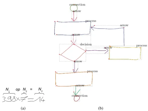
All communication is based on a fact that participants share conventions that determine how messages are constructed and interpreted. For graphical communi-cation these conventions indicates how arrangements, or layouts, of graphical ob-jects encode information. For instance, graphical languages (sketch, mathematical or chemical expressions, etc.) are composed of a set of symbols within some con-straints. These constraints could be the grammar of this language, the layout of symbols, and so on. Furthermore, the symbols are also composed of a layout of strokes. The layout means that elements (symbols, strokes) are arranged in the two dimensional space, so that we can build a coherent document. Fig. 2.6 illustrates two handwritten documents, a handwritten mathematical expression and a hand-written flowchart. Spatial relations specify how these elements are located in the layout.

(a) (b)

Figure 2.6: Two different handwritten graphical documents: (a) a handwritten math-ematical expression, (b) a handwritten flowchart.

As an example, suppose that we have a set of two different shapes of strokes called graphemes {\, /}. We assume that these graphemes are well detected by a clustering algorithm as discussed in Chapter3. Using these two graphemes, we can compose two different symbols:“∧” and “∨”. A difference between “∧” and “∨” is the spatial relation; “\” is put on the right side in “∧” and on the left side in “∨”. These spatial relations, left and right, are easily defined manually.

(27)

With more graphemes and more spatial relations, it is possible to design new symbols. For instance, using a set of graphemes {\, −, /}, we can compose a sym-bol “∀” with three strokes “\(1)”, “−(2)”, and “/(3)”. We can say “−(2)” is between “\(1)” and “/(3)”. In this case, between implies a relationship among three strokes, which is a cardinality of this spatial relation [25]. In this work, we limit the cardinal-ity of spatial relation to two strokes, from a reference stroke to an argument stroke. However, with only three strokes, we have to consider six different stroke pairs to envisage all appropriate alternatives, for example “\(1) → −(2)”, “−(2) → \(1)”, “\(1) → /(3)”, etc. The number of spatial relation couples will grow rapidly with an increasing number of strokes in the layout [26].

A traditional modeling of spatial relation is represented at three levels [25,27]: topological relations, orientation relations, and distance relations. The topological characteristics are preserved under topological transformations, for example trans-lation, rotation, and scaling [28]. The orientation relations calculate directional information between two strokes [29]. For instance a stroke A is on the right of another stroke B. The distance relations describe how far two strokes are.

Most of existing systems dealing with handwriting need some spatial relations between strokes. For instance, [29] uses a fuzzy relation position (orientation re-lations) for an analysis of diacritics on on-line handwritten text. In [30], authors add a distance information to design a structural recognition system for Chinese characters. In the context of handwritten mathematical expression recognition in [31,32], authors use the three levels of spatial relations to create a Symbol Relation Tree (SRT) using six predefined spatial relations: inside, over, under, superscript, subscript and right. Spatial relations are also useful in automatic symbol extrac-tion as in our work [26, 33]. In short, we automatically extract graphical symbols from a graphical language with a simple set of predefined spatial relations. Our ap-proach was successfully tested on a simple mathematical expression database. We predefined three domain specific relations (right, below, and intersection) to create a relational graph between strokes. The creation of this relational graph starts with the top-left stroke because of the left to right handwriting orientation. In the rela-tional graph, repetitive sub-graphs composed of graphemes and predefined spatial relations are considered graphical symbols.

(28)

describing “a new” (or “an unknown”) complex graphical language. We may lose some unknown spatial relations which are important for a specified graphical lan-guage. Let us consider differences between 9 different layouts of the 2 previous strokes {\, /}: “\/” “∨”, “/\”, “∧”, “ ”, “<”, “ ”, “>” and “×”. We want to distinguish these 9 layouts. We assume “\” as the reference stroke and “/” as the argument stroke. If we categorize these layouts by intersection, two groups will be obtained: {“\/”,“/\”, “ ”, “ ”} and {“∨”, “∧”, “<”, “>”, “×”}. If we cat-egorize these layouts by four predefined directions (right, left, above, and below) of “\”, four groups will be obtained: {“\/”,“∨”}, {“∧”, “/\”}, {“ ”, “<”}, and {“ ”, “>”} with the confusing layout “×”. The combination of left (directional relations) and intersection (topological relations) allows the distinction of these 9 layouts. However, there are many combinations of spatial relations in a complex graphical language. It is hard to manually predefine all the useful combinations of spatial relations.

As mentioned in this section, topological relations, orientation relations, and distance relations are the three levels of traditional modeling of spatial relation. In order to understand this traditional modeling, we will introduce the three levels of spatial relations in the next three sub-sections.

2.2.1 Distance Relations

A distance relation denotes how far apart two objects are. In a simple case, we can assume that two objects are considered as two points pt1 = (x1, y1) and pt2 = (x2, y2). In analytic geometry [34], the distance between two points is given by the Euclidean distance:

dist(pt1, pt2) = p

(x1− x2)2− (y1− y2)2. (2.3)

However, when two objects are very near, their shapes cannot be ignored. Each object in on-line handwriting is a set of points. To describe how far apart two objects are, we need a distance between two point sets. The Hausdorff distance HD(., .) is a metric between two point sets obji = {pti} and objj = {ptj} [35]:

(29)

where hd(objx, objy) = max ptx∈objx

min pty∈objy

(dist(ptx, pty)). Nevertheless in general, Hausdorff distance is used for matching two pattern shapes instead of measuring how far apart two objects are. In this thesis, we will meet many graphical symbols arrows which connect symbols. If the Hausdorff distance is used, it will generate a large distance. We prefer a distance by choosing the closest point pair CP P (., .) between two point sets:

CP P (obji, objj) = min pti∈obji

min ptj∈objj

(dist(pti, ptj)). (2.5)

Fig.2.7shows an example for explaining why we choose the closest point pair. Three graphical symbols in a flowchart are illustrated in Fig. 2.7. For a logical, or functional interpretation of this flowchart, from the circle symbol we have to move to the arrow and then to the rectangle. To obtain this sequence, it will be necessary to consider that the arrow is closer to the circle than the rectangle. It will be the case if CPP( , ) is used as the distance instead of HD( , ) since

CP P (“Circle”, “Arrow”) < CP P (“Circle”, “Rectangle”) (2.6)

while

HD(“Circle”, “Arrow”) > HD(“Circle”, “Rectangle”), (2.7)

we can choose “Arrow” as the next symbol.

Arrow Circle

Rectangle

Figure 2.7: Which is the closest symbol from the symbol “Circle”?

In the next section, we will introduce orientation relation describing directional information between objects.

(30)

2.2.2 Orientation Relations

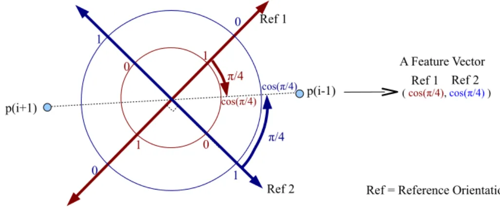
Orientation represents some directional information, e.g. east, west, south, north, etc. We can say a symbol is located at the south side of another symbol [25]. In this section, we will introduce a fuzzy directional relation between two graphical symbols [29, 36]. Ref. [29] shows that the directional relation not only depends on the positions of two symbols, but also on the shapes of two symbols.

In a fuzzy directional relation, we have to define a reference symbol R and an argument symbol A with respect to a reference direction −→uα. The angle function varying in the boundary [0, π] is defined by:

β(P, Q) = arccos( −→ QP · −→uα

||−→QP ||

) (2.8)

where β(P, P ) = 0. Thus taking an argument point P into account, we use the minimum value βminamong all the reference points Q ∈ R for defining a directional angle:

βmin(P ) = arg min Q∈R

||β(P, Q)||. (2.9)

In order to normalize it from [0, π] to [0, 1], a simple linear function is applied:

µα(R)(P ) = max(0, 1 −

2βmin(P )

π ). (2.10)

Considering the whole argument point set A, we can accumulate µα(R)(P ) for all the points, and then normalize it. Thus, we can compute a relative direction value

MR

α(A) between a reference symbol R and an argument symbol A, with respect to

a reference direction−u→α: M_αR(A) = 1 |A| X x∈A µα(R)(x). (2.11)

Taking a reference symbol “2” comparing an argument symbol “5” as an exam-ple in Fig.2.8 and a reference point P , we search for the minimum β angle. After that, we accumulate µα(R)(P ) for all the points in an argument symbol A using Eq. (2.11).

(31)

P

Q

R

Q

1

P

Q

₂

Q

₁

P

Q

₂

Figure 2.8: Fuzzy relative directional relationship from a reference symbol to an argument symbol with respect to a reference direction in Ref. [29].

In images, each object is composed of pixels. Two consecutive points in each stroke is connected. Nevertheless in on-line handwriting, in each stroke, two consecutive discrete points have some space between them according to resampling frequency. Ref. [29] points out that using Eq. (2.9) between two consecutive points will gener-ate a “comb effect”.

In order to avoid this effect, Ref. [29] redefines β (see Eq. (2.9)) from ~uα to −→

QP by the counter-clockwise direction. Hence, β is located in the range [0, 2π]. Considering a stroke composed of only one point, we just use the original definition β shown in Eq. (2.9). Usually a stroke are composed of several points. Each time, we consider a pair of consecutive points. We go through all the pairs of consecutive points Q1 and Q2 to compute two angles β1 and β2 respectively. If one β is in [0, π/2] while the other is in [π/2,3π₂ ], βmin(P ) will be zero. Otherwise, βmin(P ) will be computed as usual using Eq. (2.9).

Fig.2.9 shows two general cases for β computation. The first case is when β2 is in the range [0, π/2] while β1 is in the range [π/2,3π₂ ] on left side of Fig. 2.9. It means P is located between two consecutive points at the reference direction ~uα side. It implies that there is a middle point between Q1 and Q2. The middle point makes that βmin(P ) = 0. The second case is that both β are in the range [π/2,3π₂ ] and then βminis computed as usual using Eq. (2.9).

In this subsection, the orientation relation have been introduced. In the next section, we will study the last topological relation.

(32)

SPATIAL RELATIONS 23 P Q R Q₁ P Q₂ Q₁ P Q₂

Figure 2.9: New β function to avoid a comb effect Ref. [29]

2.2.3 Topological Relations

The topological characteristics are preserved under topological transformations for example translation, rotation, and scaling [28]. A simple example of topological relation in Fig.2.10is the intersection of two strokes.

Intersection 1. Translation 2. Rotation 3. Scaling Topological transformations

Figure 2.10: Topological transformations

To automatically generate topological relations, [37] develops formal catego-rization of binary topological relations between regions, lines, and points. Given a geometric object A, we can define the set-theoretic closure as A, the

bound-ary as ∂A, the exterior A− = U − A (where U is the universe), and the interior

A◦ = A − ∂A. A could be any geometric object, e.g. regions, lines, points, etc. In on-line handwriting, we will analyze spatial relations between strokes (lines). We use an example for explaining how to categorize binary topological relations between two lines. Eq. (2.12) shows a binary relation matrix between two objects (lines) A and B where ∅ means no intersection between them while they are inter-sected using ¬∅. Fig.2.11shows a corresponding topological relation between two lines. Ref. [37] deduces 33 relations which can be realized between simple lines

(33)

using the binary relation matrix. B◦ ∂B B− A◦ ∂A A−      ¬∅ ∅ ¬∅ ∅ ∅ ¬∅ ¬∅ ¬∅ ¬∅      (2.12) A B

Figure 2.11: Corresponding topological relations between two lines in [37]

In our work [38], we first define spatial relation features at the three levels, and then use a clustering technique to discover spatial relations rather than some predefined spatial relations. The learned spatial relations (edges) are applied to discover the graphical symbols in relational graphs. In the next section, we will discuss the clustering techniques which will be used to generate spatial relation prototypes and to generate graphical symbol prototypes.

2.3 Clustering Techniques

It exists many clustering methods in the state of the art: k-means [39],

Self-Organizing Map (SOM) [40], Neural Gas (NG) [41], Growing Neural Gas (GNG),

hierarchical clustering [42], etc. The clustering algorithm k-means consists in iter-atively seeking k mean feature vectors (prototypes), and then n samples are parti-tioned into k clusters in which each sample belongs to the cluster with the nearest prototype (center). The sample space is divided into Voronoi cells. However, the k prototypes are independent from each other. SOM, NG, and GNG contain some topological relationships between prototypes. SOM, a kind of artificial neural net-work, can produce a discretized representation as a fixed lattice in a low-dimension (typically two-dimension) space of the input space of training samples. We can see the lattice as a map for data visualization. Rather than the fixed lattice, NG

(34)

CLUSTERING TECHNIQUES 25

has a more flexible topological relationship between prototypes. In the fixed lat-tice, neighbors of a prototype are fixed while neighbors of a prototype in NG can be changed. A modified version of NG is GNG whose prototype number can be changed. It starts with a small prototype number, and prototypes could be added or be removed in each iteration. Hierarchical clustering seeks to build a hierarchy of clusters. Two general approaches exist: agglomerative (bottom up) and divisive (top down). Divisive clustering is conceptually more complex than agglomerative clus-tering [43]. In this thesis, only two clustering techniques will be used, k-means for spatial relation learning and agglomerative hierarchical clustering for multi-stroke symbol learning. In the next section, k-means will be presented in detail.

2.3.1 K-Means

The algorithm k-means is seeking k mean vectors (prototypes) M = (µ1, µ2, ...µk), which correspond to k classes, Ω = {C1, C2, ...Ck}. We assume n samples X = (x1, x2, ..., xn) and know the number of clusters k in advance. Firstly, k samples are randomly selected for the cluster centers to initialize the k-means iterative proce-dure. For each iteration, we have to update each sample membership and recalculate the prototypes M .

In order to simplify the description of this problem, only the square Euclidean distance has been considered. We define the membership function P (Ci|xp) that determines whether xp ∈ X belongs to the class Ci with the mean vector µi using the nearest squared Euclidean distance ||xp− µi||2.

P (Ci|xp) =      1 if µi = arg min µj∈M ||xp− µj||2 0 otherwise (2.13)

Eq. (2.13) is applied for allocating each sample for its cluster. After each sample gains a cluster, we have to update all the mean values M using an iterative equation Eq. (2.14). µi = n P k=1 P (Ci|xk)xk n P k=1 P (Ci|xk) (2.14)

(35)

1. Begin.

2. Initializing a number of clusters k, and (M = µ1, µ2, ...µk) randomly.

3. Allocating all the samples with its cluster using the square Euclidean metric via Eq. (2.13).

4. Updating mean values via Eq. (2.14).

5. If mean values are changed, we go to the step 3. 6. End.

Consequently, k prototypes are attained until means values are stable. The algo-rithm k-means can be easily implemented. Once we embed data into a fixed-length feature space, k-means can be used for clustering. In the next section, we will introduce agglomerative hierarchical clustering.

2.3.2 Agglomerative Hierarchical Clustering

Rather than embedding data into a fixed-length feature space, agglomerative hi-erarchical clustering require only a pair-wise distance matrix between all the data. It starts a clustering procedure with singleton clusters; every single data is a cluster. Given data X = {x1, x2, ..., xn}, each of them is a cluster Ω = {C1, C2, ..., Cn}

where Ci = {x}. The algorithm of agglomerative hierarchical clustering is

de-scribed as: 1. Begin.

2. Searching for the cluster pair with the closest distance, (i, j) = arg min Ci,Cj∈Ω

dist(Ci, Cj). 3. Merging two sets Ci and Cj becomes a new cluster Ck, and Ω = (Ω − Ci −

Cj) ∪ Ck.

4. Return to the step 2 until clustering results satisfy a criterion. 5. End.

In this algorithm, dist(Ci, Cj) represents a distance between two clusters. At the end, we will get a dendrogram that records each distance when two clusters are merged. In this thesis, six distances will be used, Single, Average, Complete, Centroid, Median, and Ward.

(36)

1. Single: Single metric computes the smallest distance between two clusters.

dist(Ci, Cj,0Single0) = min x∈Ci,x0∈Cj

||x − x0|| (2.15)

2. Average: Average metric computes the average distance between two clusters.

dist(Ci, Cj,0Average0) = 1 ninj min x∈Ci,x0∈Cj ||x − x0|| (2.16)

3. Complete: Complete metric computes the largest distance between two clus-ters.

dist(Ci, Cj,0Complete0) = max x∈Ci,x0∈Cj

||x − x0|| (2.17)

4. Centroid: Centroid metric computes the Euclidean distance between the cen-troids of two clusters.

dist(Ci, Cj,0Centroid0) = ||m(Ci) − m(Cj)|| (2.18)

where m(Ci) = _|C1_i_| P

x∈Ci

x.

5. Median: Median metric computes the Euclidean distance between weighted centroids of two clusters.

dist(Ci, Cj,0M edian0) = ||˜x − ˜x0|| (2.19) where ˜x is created by a fusion of two clusters p and q and ˜x is recursively defined as:

˜

x = 1

2(˜xp+ ˜xq) (2.20)

6. Ward:

Warduses an increase of sum of squares as a result of joining two clusters.

dist(Ci, Cj,0W ard0) = s

2|Ci||Cj| (|Ci| + |Cj|)

||m(Ci) − m(Cj)|| (2.21)

In this thesis, we will use these six metrics for grouping multi-stroke symbols. In the next section, two criteria will be introduced for evaluating clustering results.

(37)

2.3.3 Evaluating Clusters

After generating clusters, we need measures for evaluating quality of the dis-tances mentioned in this chapter. A better clustering method should attain a high intra-cluster similarity and a low inter-cluster similarity. In this thesis, we will apply both Purity and Normalized Mutual Information (NMI) [43,44] for quality assess-ment.

We accumulate the biggest numbers of major class in each cluster, and Purity is equal to a ratio of the sum of accumulation and the total data number. A for-mal definition of Purity is described as following. Given a set of clusters Ω = {w1, w2, ..., wnp} and a set of classes C = {c1, c2, ..., cJ}, Purity is defined by:

purity(Ω, C) = 1 N X wk∈Ω max cj∈C |wk∩ cj|, (2.22)

where N is the number of all the data (symbols). We can see that more clusters, and a higher purity. Singleton clusters reach the highest purity of 1.

Rather than a simple criterion Purity, NMI will be penalized by an increasing number of clusters. NMI is defined by:

N M I(Ω, C) = I(Ω; C)

[H(Ω) + H(C)] /2. (2.23)

I is the mutual information between Ω and C1_{defined by:}

I(Ω; C) = P wk∈Ω P cj∈C P (wk∩ cj) log P (wk∩cj) P (wk)P (cj) = P wk∈Ω P cj∈C |wk∩cj| N log N |wk∩cj| |wk||cj| (2.24)

where N is the number of all the symbols, and P (wk∩ cj) denotes a probability of a symbol being in the cluster wk and in the class cj (the intersection of wkand cj). H is the entropy as defined by:

H(Ω) = − P wk∈Ω P (wk) log P (wk) = − P wk∈Ω |wk| N log |wk| N . (2.25)

NMI in Eq. (2.23) is in a range between 0 and 1 [43]. NMI= 0 means a random

(38)

choice on classes. A higher value is preferable. We can see that NMI in Eq. (2.23) is normalized by [H(Ω) + H(C)]/2, a function in terms of the cluster number where H(C) is invariant with the cluster number and H(Ω) reaches the maximum value log N for np = N .

However, for two clustering results with the same number of clusters |Ω1| = |Ω2|, a higher Purity(P urity(Ω1, C) > P urity(Ω2, C)) does not mean a higher NMI. It is possible that: N M I(Ω1, C) < NM I(Ω2, C).

For example, Fig.2.12displays |Ω1| = 3 clusters containing digits with |C| = 3 labels (classes), C = { “2”, “4”, “7” }. In total, there are N = 18 instances of symbol.

Cluster 1 Cluster 2 Cluster 3

Figure 2.12: Example of three clusters for three classes (three handwritten digits “2”, “4”, and “7”)

Puritycan be easily computed by:

P urity(Ω1, C) =

4 + 5 + 4

18 = 0.72, (2.26)

and the mutual information between Ω1 and C is defined by:

I(Ω1; C) = 1 18(4 × log 18 × 4 6 × 6 + 1 × log 18 × 1 6 × 6 + 1 × log 18 × 1 6 × 6 +1 × log18 × 1 7 × 6 + 5 × log 18 × 5 7 × 6 + 1 × log 18 × 1 7 × 6 +1 × log18 × 1 5 × 6 + 0 + 4 × log 18 × 4 5 × 6 ) = 0.33. (2.27)

The entropies of Ω1 and C are computed by:

H(Ω1) = −1 × 6 18log( 6 18) − 1 × 7 18log( 7 18) − 1 × 5 18log( 5 18) = 1.57, (2.28)

(39)

and H(C) = −1 × 6 18log( 6 18) − 1 × 6 18log( 6 18) − 1 × 6 18log( 6 18) = 1.59. (2.29)

At the end, the normalized mutual information is obtained by:

N M I(Ω1, C) =

0.33

(1.57 + 1.59)/2 = 0.21. (2.30)

Fig.2.13 shows two distribution matrix for two clustering results respectively. The example in Fig.2.12is represented by the distribution matrix in Fig.2.13a. We change the distribution from Ω1 to Ω2 in Fig.2.13b by keeping 3 clusters. Purity and NMI are obtained in Fig. 2.13c. The scatter non-major classes result in lower N M I(Ω1, C) even Ω1 has a higher purity.

Ω₁ 1 2 3 4 1 1 1 5 1 1 0 4 Ω₂ 1 2 3 4 1 0 3 5 2 0 0 3 (a) (b) Ω₂ Ω₁ Purity NMI (c) 0.67 0.37 0.21 0.72

Figure 2.13: Two clustering results (a) and (b) with a same number of 3 clusters

In the next section, we will present relative works on generating a codebook in handwriting using clustering. The interest of this codebook, when available, is to allow the user to manually labeled each symbol, eventually containing several strokes, and then to propagate this labeling to the raw data.

2.4 Codebook Extraction in Handwriting

In this section, we discuss the codebook generation at two levels: the single-stroke symbol level and the multi-single-stroke symbol level.

Extracting a codebook from single strokes in the field of both offline and on-line handwriting has gained increased attention. Many offline biometric systems [45–

(40)

CONCLUSION 31

map, etc.) so that a codebook-based probability distribution function can be em-ployed to identify or verify the writers. It is necessary to cut the offline ink (to segment it) beforehand [45,46], then basic components are extracted for generating the codebook. In these cases the codebook aims to be representative of a writer, but not to match to language symbols. Considering the on-line handwriting, basic elements are the strokes, so we can build directly a codebook at the single-stroke level in this thesis.

A multi-stroke codebook based on the k-means algorithm is built in [39] for clustering the different allographs of the same letter but beforehand a complete seg-mentation and recognition tool is applied on the text document. Varied features are used for this clustering. The two-dimensional graphical symbols containing sev-eral strokes are re-sampled into a fixed number of points, and then embedded in a feature vector space so that we can compute a distance between two graphical symbols. However, the order of strokes has not been discussed; the embedding is stroke-order-sensitive. We need a stroke-order-free algorithm to obtain the dis-tance between two graphical symbols composed of many strokes; writers may copy a same symbol with different stroke orders and different stroke directions. More-over, segments comprising different numbers of strokes would be the same symbol (stroke-number-free problem). In our work, we make use of a Modified Hausdorff Distance (MHD), which is widely used in contour matching on offline data (im-ages) [35, 48], in order to avoid the problem of stroke-order, stroke-direction, and stroke-number (see Section3.5.3in detail).

After codebook generation, we have to manually label symbols. [14, 15] only give a label to a correctly segmented character. In reality, it is difficult to build clusters that contain only well segmented symbols. Many clusters would mix the symbols with the sub-parts of other symbols. We have to create a symbol mapping from labeled symbol instances to raw symbol instances. Furthermore, we need a criterion for evaluating how much work we have been reduced.

2.5 Conclusion

Building the ground-truth dataset at the symbol level is a tedious work. Two main steps exist in the ground-truth dataset creation: symbol segmentation and

(41)

sym-bol labeling. We propose to organize the graphical language as relational sequences and relational graphs. The MDL principle on sequences and on graphs have been presented to automatically generate the symbol segmentation. We can group seg-mented symbols into a codebook using clustering algorithms. A codebook will be generated so that we can label symbols at the codebook level, which can save sym-bol annotation workload. In the next chapter, we start to discuss several similarities between two isolated symbols and symbol quantization using hierarchical cluster-ing. The multi-stroke symbol codebook can be generated for labelcluster-ing.

(42)

3

Quantifying Isolated Graphical

Symbols

As every instance of a handwritten graphical symbol is different one from the other because of the variability of human handwriting, it is of prime importance to be able to compare two patterns and further more to define clusters in the feature space of patterns which are very similar. In this chapter, we introduce a hierar-chical clustering which is convenient in a context of unsupervised clustering. This clustering algorithm requires a pairwise distance matrix between all the graphical symbols. We mainly discuss a distance between two graphical symbols which are two sets of sequences. According to the composition of graphical symbol, we can divide discussion into two categories, a distance between two single-stroke symbols and a distance between two multi-stroke symbols. With respect to the first category, the famous Dynamic Time Warping (DTW) based distance allows an elastic match-ing between two strokes. It is considered as an efficient algorithm for smatch-ingle stroke patterns. To deal with multi-stroke patterns, a first solution consists in a simple con-catenation of the strokes respecting a natural order, which is most of the time the temporal order. However, as we will see with some examples introduced later in this chapter, this solution is not always satisfying. To allow more flexibility in the

(43)

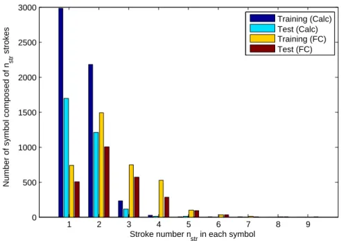
struction of the stroke sequence we will propose a novel algorithm, called DTW-A* (DTW A star). As it turns out to be a very time consuming method, we have also proposed a modified Hausdorff distance (MHD) to allow even more flexibility in the matching process while reducing the computation time. In that last case, all the temporal constraints of the point sequences are ignored. To analyze the behavior of these distances and of the hierarchical clustering algorithm, two datasets have been considered. One is the Calc dataset, it is composed of single line mathematical ex-pressions, the second one is more challenging, it is the FC dataset with handwritten flowcharts.

3.1 Introduction

In on-line handwriting, basic elements are strokes. Each stroke contains a se-quence of points, from a pen-down point to a pen-up point. Hence, the stroke is oriented. A graphical symbol is composed of one or several strokes. To automat-ically quantify graphical symbols, a clustering technique is required for grouping symbol shapes. As reminded in the state of the art section, it exists many clustering methods, hierarchical clustering [42], k-means [39], self-organizing map [40, 49], neural gas [41], etc. For implementing the clustering, a common necessary condi-tion is to be able calculate a distance (or a similarity) between two symbols. In this chapter, we will discuss the distance between two isolated multi-stroke graphical symbols, equivalently between two sets of point sequences.

Different people may write a visually same symbol with different stroke direc-tions and different stroke orders. In writer identification, these characteristics can efficiently distinguish writers [39]. However, to understand or communicate the same symbol written by different writers, stroke direction and stroke order should be ignored. We human read handwritten symbols without knowing the stroke direc-tion and the stroke order. For instance, a symbol containing a horizontal stroke “−” can be written by two different approaches, from left to right “→” or an inverse way “←”.

DTW (Dynamic Time Warping) is an algorithm which computes a distance be-tween two single-stroke symbols. It obeys a continuity constraint and a boundary constraint during point-to-point matching [12]. These two constraints will be

(44)

elabo-INTRODUCTION 35

rated in Section3.4.1. Comparing two opposed direction strokes, the distance DTW distDT W(→, ←) naturally produce a large value because of two inverse directions. A simple solution is to choose the smallest distance between two possible direc-tions of one stroke: min(distDT W(→, ←), distDT W(inv(→), ←)) where inv(.) is an operator of reversing stroke trajectory direction.

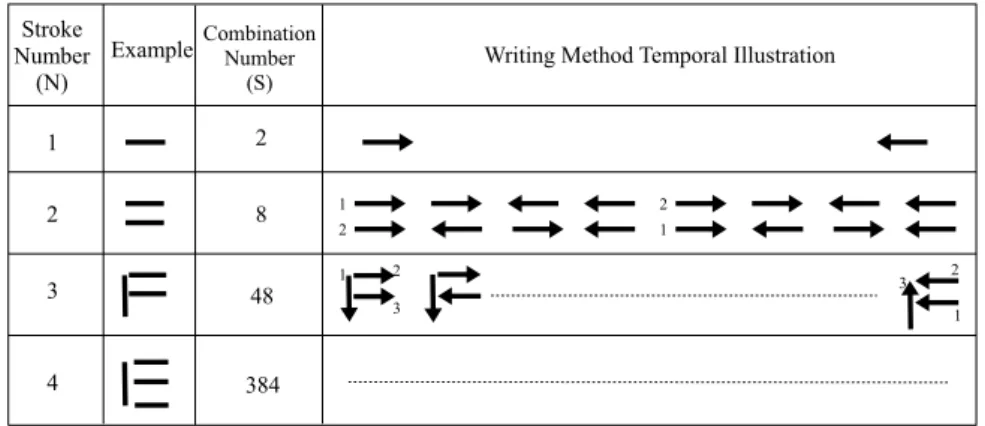
However, when comparing two multi-stroke symbols, the number of possible di-rections and orders increases very fast in terms of a growing stroke number. Tab.3.1

illustrates an example of how to write “E” within four strokes. With this example, 384 different writing sequences are possible. This example shows the complexity of combinations of different stroke directions and stroke orders. In general, the number of different temporal writing ways for a symbol is given by:

SN = N ! × 2N = 2 × N × S(N −1) (3.1)

where N is the stroke number of a symbol. For calculating the distance DTW between two multi-stroke symbols, a simple solution is to concatenate the strokes using different stroke directions and stroke orders.

1 2 2 1 2 1 3 2 1 3 Stroke Number (N)

Example Combination_Number (S)

Writing Method Temporal Illustration

1 2 3 4 2 8 48 384

Table 3.1: Variability of stroke order and direction in an on-line handwritten symbol

For example, for the distance DTW between

1 2 2 1 2 1 3 2 1 3 (4 strokes) and 1 2 2 1 2 1 3 2 1 3 (2 strokes), we should calculate 384 × 8 = 3092 possible combinations. This large combina-tion number is due to different writing orders of N strokes (N !) and due to the two directions of each written order (2N).

In a more extreme case, we can get rid of all the temporal information and con-sider the symbols as a set of points ignoring the sequences they produce. This leads to use the Hausdorff distance [35]. This metric is used in image processing domain

Symbol and Spatial Relation Knowledge Extraction Applied to On-Line Handwritten Scripts

HAL Id: tel-00785984

https://tel.archives-ouvertes.fr/tel-00785984

Applied to On-Line Handwritten Scripts

Jinpeng Li

To cite this version:

Thèse de Doctorat

Jinpeng Li

Extraction de connaissances symboliques et

relationnelles appliquée aux tracés manuscrits

structurés en-ligne

Acknowledgements

Contents

1

Introduction

Expressions

Relational Graphs

"+"

"+"

Legend

Relational Graphs

"="

"="

Segmentation

I: Intersection

R: Right

B: Below

"5"

"5"

(.): Stroke Index

2

State of the Art

2.1

Symbol Segmentation Using the MDL principle

2.1.1

A Sequence Case

2.1.2

A Graph Case

R

I

R

R

B

R

R

I

R

B

R

R

R

"="

"="

Codebook

a

Shape

Label

b

c

d

e

R

I

R

R

R

R

I

R

R

R

R

"="

"="

R

R

B

Lexical unit "=" : I(u)=3

I(G|u)=26

I(G)=30

_I

_B

_I

_I

_I

_I