HAL Id: hal-00017990
https://hal.archives-ouvertes.fr/hal-00017990
Submitted on 26 Jan 2006
HAL is a multi-disciplinary open access
archive for the deposit and dissemination of
sci-entific research documents, whether they are
pub-lished or not. The documents may come from
teaching and research institutions in France or
abroad, or from public or private research centers.
L’archive ouverte pluridisciplinaire HAL, est
destinée au dépôt et à la diffusion de documents
scientifiques de niveau recherche, publiés ou non,
émanant des établissements d’enseignement et de
recherche français ou étrangers, des laboratoires
publics ou privés.
clouds
Valentine Wakelam, Eric Herbst, Franck Selsis
To cite this version:
Valentine Wakelam, Eric Herbst, Franck Selsis. The effect of uncertainties on chemical models of dark
clouds. Astronomy and Astrophysics - A&A, EDP Sciences, 2006, in press, in press. �hal-00017990�
ccsd-00017990, version 1 - 26 Jan 2006
Astronomy & Astrophysicsmanuscript no. aa-incertcloud.hyper19319 January 26, 2006 (DOI: will be inserted by hand later)
The effect of uncertainties on chemical models of dark clouds
V. Wakelam
1, E. Herbst
1,2
, F. Selsis
31 Department of Physics, The Ohio State University, Columbus, OH 43210, USA 2
Departments of Astronomy and Chemistry, The Ohio State University, Columbus, OH 43210, USA
3 Centre de Recherche Astronomique de Lyon, Ecole Normale Sup´erieure, 46 All´ee d’Italie, F-69364 Lyon cedex 7, France
Received xxx / Accepted xxx
Abstract. The gas-phase chemistry of dark clouds has been studied with a treatment of uncertainties caused both by errors in individual rate coefficients and uncertainties in physical conditions. Moreover, a sensitivity analysis has been employed to attempt to determine which reactions are most important in the chemistry of individual species. The degree of overlap between calculated errors in abundances and estimated observational errors has been used as an initial criterion for the goodness of the model and the determination of a best ‘chemical’ age of the source. For the well-studied sources L134N and TMC-1CP, best agreement is achieved at so-called “early times” of ≈ 105
yr , in agreement with previous calculations but here put on a firmer statistical foundation. A more detailed criterion for agreement, which takes into account the degree of disagreement, is also proposed. Poorly understood but critical classes of reactions are delineated, especially reactions between ions and polar neutrals. Such reactions will have to be understood better before the chemistry can be made more secure. Nevertheless, the level of agreement is low enough to indicate that a static picture of physical conditions without consideration of interactions with grain surfaces is inappropriate for a complete understanding of the chemistry.
Key words.Astrochemistry – ISM: abundances – ISM: clouds – ISM: molecules
1. Introduction
The chemistry of dark clouds, now known as quiescent cores, has been studied for over thirty years (Herbst & Klemperer 1973; Watson 1973). Indeed, a significant frac-tion of the more than 130 gas-phase species detected via high-resolution spectroscopy in the interstellar and cir-cumstellar media has been seen in such sources, which include the well-studied clouds TMC1-CP and L134N (Smith et al. 2004; Terzieva & Herbst 1998). In an at-tempt to reproduce the abundances of these species, a large number of gas-phase chemical models have been de-veloped that compute the variation of the gas-phase con-centrations as a function of time. For many years, most of these models were based on the pseudo-time-dependent approximation (Prasad & Huntress 1980; Leung et al. 1984; Langer et al. 1984; Millar & Nejad 1985), in which the chemistry evolves under fixed and homogeneous con-ditions from some initial abundances, consisting of totally atomic material except for a high abundance of H2. In
the last decade, more complex models, including surface chemistry (Hasegawa et al. 1992; Ruffle & Herbst 2000), heterogeneity of the source (Hartquist et al. 2001), and
as-Send offprint requests to: [email protected]
sorted effects of dynamics and turbulence (Markwick et al. 2000), have been reported.
In all of these models, the connections among gas-phase species are described by up to thousands of chem-ical reactions, with rates quantified by rate coefficients, most of which are poorly determined by experimental or theoretical means. Nevertheless, even the older pseudo-time-dependent models were at least partially success-ful in reproducing the exotic nature of the chemistry (molecular ions, radicals, and metastable isomers), the unsaturated nature of the more complex products (e.g., cyanopolyynes), and the strong deuterium fractionation. They have been less successful, however, in detailed com-parisons with observations of fractional abundances and column densities for the large number of species observed in individual sources. In the last published comparison between a pseudo-time-dependent theory and observation for the well-studied source TMC1-CP (Smith et al. 2004), it was found that at the time of best agreement (1 × 10⁵
yr), only about 2/3 of the observed species have calculated fractional abundances within an order-of-magnitude of the observed values. This result, obtained with the relatively new osu.2003 network and so-called “low-metal” elemental abundances, is actually worse than obtained with a pre-vious network from the Ohio group, known as the “new standard model” (nsm), where nearly 4/5 of the molecular
abundances were reproduced to within one order of mag-nitude (Terzieva & Herbst 1998). The order-of-magmag-nitude criterion used in both studies is a subjective one, however, and no comparison involving TMC1-CP has ever been done by taking into account the rate coefficient uncer-tainties in the computation of the theoretical abundances. Without any quantification of the random model er-ror, it is difficult to conclude if observed abundances can be reproduced or not by the model. Indeed, including the estimated uncertainties in rate coefficients is the only way to define those species with abundances not reproduced by chemical networks. With a rigorous quantitative ap-proach to uncertainty, moreover, one can begin to compre-hend the deficiencies of gas-phase pseudo-time-dependent calculations, and determine where improvement is most necessary. If, for example, hydrogen-rich species, which may be synthesized on grain surfaces and desorbed into the gas via non-thermal means, are the only species with abundances to be poorly reproduced, the most important correction would involve the inclusion of surface processes. If, on the other hand, smaller species such as O2and H2O,
with simple chemistry, cannot be reproduced within the estimated errors, then it is at least conceivable that a far more complex physical scenario is needed in which the for-mation and dynamics of the quiescent core play roles in the chemistry (Bergin & Melnick 2005). Whether or not to give up on the pseudo-time-dependent approximation then depends critically on our estimates of uncertainties, because there is no point in violating Occam’s Razor if a more simple theory is as adequate as a more complex one. This paper is the second application of a method de-veloped in Wakelam et al. (2005) to quantify the random errors of chemical models. In Wakelam et al. (2005), we presented the method in great detail and showed some consequences for hot core chemistry (T> 100 K). Hot cores occur during an evolutionary stage of star forma-tion, and can have complex structures not well understood (Nomura & Millar 2004). Dark clouds, which have not yet started to collapse in an appreciable manner, may, on the contrary, have relatively simple temperature and den-sity structures. These objects are then better laboratories to test the gas-phase chemical models usually used. In this paper, we apply the method to estimate the statisti-cal errors as a function of time for dark cloud chemistry, which is occurring at an H2density of ∼ 104 cm−3 and a
temperature < 20 K. A previous analysis of uncertainties for mainly steady-state conditions was performed for dark clouds by Vasyunin et al. (2004), although their error was defined in a different manner.
The remainder of our paper is organized as follows. In Section 2, we briefly describe the chemical network and ap-proach to uncertainties used for this study. Some general results are presented in Section 3, where we also (i) con-sider differences between the two major networks, and (ii) make a comparison between our uncertainty calculations and those of Vasyunin et al. (2004). Section 4 contains a comparison between our results and observed abundances towards the two dark clouds L134N and TMC1-CP, while
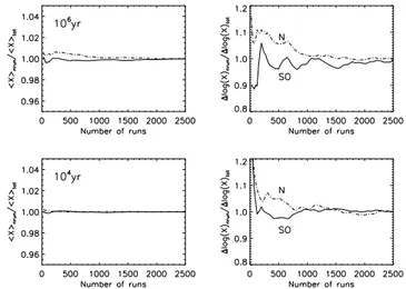
Fig. 1. Mean abundance (< X >) (left panels) and error ∆ log X (right panels) for N and SO plotted as a function of the number of runs. Both quantities are normalized by the value obtained for the maximum number of runs (2500). The results are given for Model 2 at two times: 104yr on the lower panels and 106yr on the upper panels.
Table 1.Physical parameters for the models.
Physical conditions Model 1 10 K, 104 cm−3a Model 2 5-15 K, (0.5 − 1.5) × 104 cm−3a Model 3 5-15 K, (0.5 − 1.5) × 104 cm−3a, C/O=1.2 a H2density.
Table 2.Initial elemental abundances with respect to H2.
Initial abundances He 2.8 × 10⁻¹ Fe+ 6.0 × 10⁻⁹ N 4.28 × 10⁻⁵ Na+ 4.0 × 10⁻⁹ O 3.52 × 10⁻⁴ Mg+ 1.4 × 10⁻⁸ C+ 1.46 × 10⁻⁴ P+ 6.0 × 10⁻⁹ S+ 1.6 × 10⁻⁷ Cl+ 8.0 × 10⁻⁹ Si+ 1.6 × 10⁻⁸
Section 5 discusses the specific cases of O2 and H2O, and
the cloud ages. We conclude the paper in Section 7.
2. Chemical network and uncertainty method
We used a time-independent physical model with the gas-phase chemical network osu.20031reported by Smith et al.
(2004). This network contains standard gas-phase reac-tions (ion-neutral, neutral-neutral, dissociative recombi-nation etc), with the addition of a significant number of rapid radical-neutral processes. Except for H2production,
the grains are only important as sites of negative charge that recombine with positive ions. We considered the
certainties in all the classes of reactions except for ion re-combination with negative grains. The uncertainties in the rate coefficients have recently been added to the osu.2003 network, based on those listed in the RATE99 network (Le Teuff et al. 2000)2. For the uncertainties not
esti-mated at 10 K (according to the temperature range given in RATE99), we increased the uncertainty to a factor of 2.
The Monte Carlo method used here to include the rate-coefficient uncertainties is described in detail by Wakelam et al. (2005). Briefly, it consists of generating N new sets of rate coefficients by replacing each coefficient ki by a
random value consistent with its uncertainty factor Fi.
We assume a normal distribution of log ki with a
stan-dard deviation σi = log Fi. We run the model for each
set j, which produces, for each species, N values of the abundance Xj(t) at a time t. The mean value of log X(t)
gives us the “recommended” value while the dispersion of log Xj(t) around < log X(t) > determines the error
due to kinetic data uncertainties. The error in the abun-dance ∆ log X = 1
2(log Xmax− log Xmin) is defined at a
time t as the smallest interval [log Xmin, log Xmax] that
contains 95.4% of log Xj values, which is equivalent to
2σ for symmetric Gaussian distributions. For example, if ∆ log X = 1.0 and the calculated distribution is symmet-ric, then the 2σ values of Xmaxand Xminare one order of
magnitude greater and less than X, respectively. Similarly, if ∆ log X = 0.5, the 2σ values are greater and less than X by a factor of 3.3, and if ∆ log X = 0.3, they are greater and less than X by a factor of 2.0.
We initially ran two models with different physical con-ditions. In the first model (Model 1), the temperature and the H2 density are held constant at values of 10 K and
104cm−3, respectively; only the rate coefficients vary. For
the second model (Model 2), we randomly chose the tem-perature and the density within a possible range of values. This uncertainty was adopted for two reasons: (i) the cloud temperature and density are usually derived from obser-vations (using approximate line excitation models) and an error in these values can usually be determined, and (ii) the modeled clouds are more likely to be inhomogeneous sources with contributions over the chosen ranges of tem-perature and density. We investigated the sensitivity of the results if an uncertainty of ±50% is considered for T and n(H2) around the typical values given for Model 1 (see
Table 1). Because temperature and density are physical parameters not characterized by a Gaussian distribution, we used a flat distribution instead for the rate coefficients. For both models, we used a cosmic-ray ionization rate of 1.3 × 10⁻¹⁷ s−1, a visual extinction of 10 and the
low-metal elemental abundances, which are listed in Table 2. A third model, with carbon-rich elemental abundances, is discussed later in the text.
For Model 1 and Model 2, we performed 2000 and 2500 different runs, respectively. In order to demonstrate con-vergence, we plot as examples in Fig. 1 the mean
abun-2 http://www.udfa.net C CO N2 O2 C2 OH HCS C2H2 C5 HCOOCH3 HC3N HC7N
Fig. 2. Error ∆ log X as a function of time for some species with Model 1.
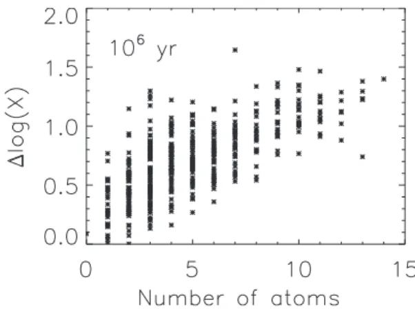
Fig. 3. Error, ∆ log X, as a function of the number of atoms per molecule at 106 yr for Model 1.
dance < X > and its error ∆ log(X) for the species N and SO as functions of the number of runs at two dif-ferent times with Model 2. The plotted parameters are normalized by the values obtained for 2500 runs. For all the species, we noticed that the number of runs chosen is more than adequate.
3. Calculated uncertainties in abundances
3.1. General considerations
Figure 2 presents the error ∆ log X for some species as a function of time and for the physical conditions of Model 1 (see Table 1). As already noticed for hot core chem-istry, the errors in the abundances increase with time for most of the molecules except the species that contain a dominant portion of an element, such as CO for carbon and N2for nitrogen. For example, the errors for HCN and
HC3N are 0.2 and 0.5 at 105 yr and increase to 0.3 and
1.1, respectively, at 107 yr. The error also increases with
the complexity of the molecule, an effect previously noted by Vasyunin et al. (2004). This effect is shown in Fig. 3 for the physical parameters of Model 1 at a time of 106
yr. For molecules with 10 atoms, the figure shows that an error of 1.0, corresponding to a factor of 10, is in the mid-dle of the range, while for molecules with five atoms, the median error is ≈ 0.7, corresponding to a factor of five.
Fig. 4.Density of probability of the NH+
4 abundance. The
right plots represent the histograms of the abundance dis-tributions at 107 yr. The top row is for Model 1 and the
bottom for Model 2.
Fig. 5. Error, ∆ log X, as a function of the number of atoms per molecule at 106 yr for Model 2.
3.2. Variation of the temperature and density
The variations of the gas temperature and density in Model 2 cause two major effects. First, they modify the distribution of the abundances at a given time from a Gaussian shape to an asymmetrical one, as can be seen by the example of NH+4 in Fig. 4. The effect is not surprising
since the rate equations are not linear with respect to den-sity or temperature. Indeed, the dependence on tempera-ture can be exponential for processes with a small barrier. The second effect is an increase in the error, which can be significant for some of the species, as shown in Fig. 5, which is to be compared with Fig. 3. The nitrogen-bearing species are particularly sensitive to the variation of tem-perature and density, as can be seen by the examples in Table 3. What causes this extreme sensitivity? It is likely
Table 3. Examples of errors computed using Model 1 (∆ log X1) and Model 2 (∆ log X2) at 105yr.
Species ∆ log X1 ∆ log X2 N+ 0.36 1.0 HNO 0.31 0.91 NH3 0.27 0.88 NH2CN 0.37 0.87 SO 0.64 0.79 H2O 0.40 0.42 HC3N 0.45 0.56 C9N 0.43 0.53
that the variation in temperature is the cause because the nitrogen chemistry starts with the reaction N+ + H
2 →
NH++ H, which is assumed to be endothermic by 85 K in
both the osu.2003 and RATE99 networks. The situation is more complex than can be contained in networks because it is likely that an estimated non-thermal fraction of H2
in its J=1 ortho state of 10−3 drives the reaction and
es-sentially converts all the atomic nitrogen ion into NH+
(Le Bourlot 1991). Nevertheless, with the adopted rate coefficient, the reaction to form NH+ is so inefficient at
temperatures under 10 K that it loses importance. Thus, temperatures lower than 10 K lead to much lower abun-dances for some N-bearing species. The result is a skew-ing of the abundance distributions to lower values, as can be seen for the case of NH+
4 in Fig. 4. The effect of the
temperature and density variations is less important for complex molecules because the variations caused by the physical parameters are diluted by the large uncertainties due to the uncertainties in rate coefficients. For example, the uncertainties in the cyanopolyne abundances do not show a strong dependence on the physical parameters: the increase of ∆ log X with Model 2 is less than a factor of 2 for HCN and this number decreases with the increasing complexity of the cyanopolyne.
3.3. Comparison between osu.2003 and RATE99
databases
The statistical uncertainties in the rate coefficients are not the only sources of error for gas-phase models. Most of the reactions have not been studied in the laboratory or via detailed theoretical considerations, so that approximate values for the rate coefficients must be used. Even studied reactions, if studied by more than one group, show large discrepancies in rates. Some of the problems in choosing proper rate coefficients can be seen in a comparison of the osu.2003 and RATE99 databases, which contain many reactions with different choices of rate coefficients. These differences arise from several specific sources:
a) Different estimates for poorly understood reactions such as radical-neutral reactions and both neutral-neutral and ion-molecule radiative associations, b) Different choices of experimental values from
CO RATE99 osu.2003 H2O CS Observed abundance in L134N
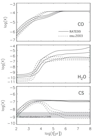
Fig. 6. CO, H2O and CS abundances as a function of
time computed using the osu.2003 (dashed lines) and the RATE99 (solid lines) databases. The three curves for each molecule and database refer to the average value and the 2σ errors.
Database (http://kinetics.nist.gov/index.php) or from competing measurements,
c) Different approximations regarding the temperature dependence of ion-polar neutral reactions.
The problem with radical-neutral reactions has been stud-ied by Smith et al. (2004): the osu.2003 network includes estimates of rapid rates for a variety of such reactions that are greater than used in RATE99 as well as the previous network from the Ohio group. The last discrepancy de-rives from the fact that although experiments show that virtually all of the small number of ion-polar neutral reac-tions studied possess an inverse temperature dependence (Rowe 1992; Rowe & Rebrion 1992) this dependence is not easily expressible in terms of the simple rate expres-sion used in the networks. Based on the work of Herbst & Leung (1986), the osu.2003 network uses an approxima-tion derived from the locked dipole approximaapproxima-tion for lin-ear neutrals and classical scaling approach for non-linlin-ear neutrals (Su & Chesnavich 1982). Both of these approxi-mations lead to a temperature dependence of T−1/2, while
the RATE99 network assumes the rate coefficients to have no temperature dependence. More detailed studies show that the inverse dependence of the rate coefficient on tem-perature may well be in between these two limiting cases
(Neufeld et al. 2005). More work is clearly needed on these systems.
At 10 K, 60% of the reactions present in both databases show a difference in rate coefficient lower than the considered uncertainty, a condition which can be ex-pressed as
ki1/ki2
√
2Fi ≤ 1,
(1) where k1and k2are the rate coefficients from the different
networks with k1> k2and F is the uncertainty factor. In
other words, almost half of the common reactions show a difference in rate coefficient not covered by the uncertain-ties in the rate coefficients, with 2% of them having an “extra” difference greater than three orders of magnitude (ki1/ki2
√
2Fi > 1000). These differences may not have strong
consequences on the modeling results, however, if the re-actions concerned are not important or if formation and depletion reactions in one model are both larger to a sim-ilar extent than in the other. So, one must ask whether or not the differences between the abundances computed with the two databases are larger than the errors due to rate coefficient uncertainties.
To answer this question, we ran Model 1 with the RATE99 network so as to compare with the osu.2003 re-sults. We obtained distributions of results for abundances that do not always overlap at the 2σ level. In fact, eighty-four percent of the 373 common species show a disagree-ment at some times between the abundances computed with the two databases. No neutral species and only 62 ions, such as S+, C+
2, CN
+ and C+
6, overlap at all times.
Note that the differences are due to difference in the val-ues of the rate coefficients and not in the differing reaction lists for the two networks, since we repeated the compari-son with a list of reactions common in both databases and obtained similar results. Fig. 6 shows three examples: the CO, H2O and CS molecules. The error in the abundance
of CO at later times is very low because this molecule is the main reservoir of atomic carbon in the gas phase and both sets of reactions give the same results. At early times, between 6 × 10³ and 2 × 10⁵ yr, the abundance
computed with osu.2003 is higher than the one computed with RATE99, reaching a ratio of 4 at 3 × 10⁴yr. The
en-velopes defined by the error in the rate coefficients do not overlap. For H2O, the early and late abundances diverge
by one order of magnitude and the envelopes do not quite overlap, whereas CS is produced to a much greater extent for the RATE99 case: the difference of up to 2 orders of magnitude at steady state far exceeds the envelopes of er-ror. Indeed, with RATE99, CS is found to be the reservoir of S: the difference between the 2 networks is thus quite profound and not only quantitative.
We attempted to identify the reason for the discrep-ancy involving CS using the sensitivity method described in Wakelam et al. (2005). At 105 yr, of the 20 most
im-portant reactions in the calculation of CS with the osu database, 10 are different in RATE99 and for those 10, 7 are ion- polar neutral reactions. If we replace these 10
rate coefficients by their values in RATE99, the CS result approaches the RATE99 abundance to within a factor of ≈ 3. Thus, one would argue that the sensitivity approach works well in deducing both the “important” reactions in the osu calculation and the reason for the difference with the results from the RATE99 calculations. But, one must be cautious because different results are obtained if one starts with RATE99: here, because of their smaller rate coefficients, ion-polar neutral reactions play a less signifi-cant role in the production and destruction of CS. Indeed, the reactions of importance for CS are quite different in the two networks. The introduction of the osu rates for a small number of ”important” reactions in the RATE99 network produces only a small change although the differ-ence in the rate coefficients of these reactions is not cov-ered by the uncertainty factor. The RATE99 abundance of CS is thus more stable against rate coefficient modifica-tions, which shows that a large number of reactions would have to be modified in order to change the result.
For CO, which shows a factor of 3 difference at early times, we were not able to identify any main reactions responsible for this discrepancy. Once again, these small differences are then due to a large number of reactions with small variations of rate coefficients between the two databases.
3.4. Comparison of uncertainty calculations
Vasyunin et al. (2004) did a similar study on dark cloud chemistry to ours using a previous version of the RATE99 database with a flat distribution for the rate errors (see Wakelam et al. 2005, for a discussion concerning this point) and focused their results on the steady-state abun-dances. Although they defined the error in the abundance in a different way, we can compare their results with ours at 108 yr. The authors used the full width at half
maximum (FWHM) of the histograms of log X, which is ∼ 2.352 ∆ log X, as defined in Sect. 2, since most of the
his-tograms have a Gaussian shape (see the discussion about the definition of the error in Wakelam et al. 2005). For most of the species, we found a lower uncertainty than did Vasyunin et al. (2004). As an example, the C4
mole-cule has a ∆ log X of 1.45 at 108 yr in our study whereas
Vasyunin et al. found an FWHM of 2-3 for carbon clusters. The reason for this difference appears to be mainly due to the database used, because we found that the errors are generally higher with RATE99 than with osu.2003, as can be seen in Fig. 6 for the case of H2O. For the specific case
of the molecule C4, we calculate that ∆ log X is 2 at 108yr
with RATE99, a value well above what we calculate with osu.2003. The source of this difference in errors is unclear.
4. Comparison with observations
We have compared our theoretical results with some ob-servations in two dark clouds: L134N (N position) and TMC-1 (CP peak). The abundances observed in L134N are summarized in Table 4 while those observed in
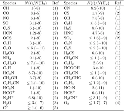
TMC-Table 4.Observed abundances towards L134N.
Species N (i)/N (H2) Ref Species N (i)/N (H2) Ref CH 1(-8) (1) CN 8.2(-10) (1) CO 8.(-5) (1) CS 1.7(-9) (2) NO 6.(-8) (1) OH 7.5(-8) (1) SO 3.1(-9) (2) C2H ≤5.(−8) (1) C2S 6.(-10) (1) H2S 8.(-10) (1) HCN 1.2(-8) (2) HNC 4.7(-8) (2) OCS 2.(-9) (1) SO2 ≤1.6(−9) (2) C3H 3.(-10) (1) C3N ≤2.(−10) (1) C3O ≤5.(−11) (1) C3S ≤2.(−10) (1) H2CO 2.(-8) (1) H2CS 6.(-10) (1) NH3 9.1(-8) (1) CH2CN ≤1.(−9) (1) C2H2O ≤7.(−10) (1) C3H2 2.(-9) (1) C4H 1.(-9) (1) HCOOH 3.e-10 (1) HC3N 8.7(-10) (2) CH3CN ≤1.(−9) (1) CH3OH 3.7(-9) (2) CH3CHO 6.(-10) (1) C2H3CN ≤1.(−10) (1) C3H4 ≤1.2(−9) (1) HC5N 1.(-10) (1) HC7N 2.(-11) (1) HCO+ 1.(-8) (2) HCS+ 6.(-11) (1) N2H+ 6.8(-10) (2) H2CN+ ≤3.1(−9) (1) H2O ≤3.(−7) (3) O2 ≤1.7(−7) (4) C0 ≥1.(−6) (5) a a(−b) refers to a × 10−b (1) Ohishi et al. (1992) (2) Dickens et al. (2000) (3) Snell et al. (2000) (4) Pagani et al. (2003) (5) Stark et al. (1996) OH Observed abundance CH3OH dCH 3OH
Fig. 7. Theoretical abundance of OH (left) and CH3OH
(right) as a function of time for Model 2. The dashed lines represent the observed values in L134N with an error of a factor of 3. The agreement between the observed and modeled abundance of OH is shown as a dark area whereas the disagreement for CH3OH is quantified by a distance
of disagreement d (see Sect. 5.2).
1CP are listed in Smith et al. (2004, Table 3). The goal of this comparison is to take into account both the uncer-tainty in the observed values and in the chemical model-ing. For the observed abundances, since all the abundances are not given with their corresponding errors, we assumed a standard uncertainty of ± a factor of 3 for the follow-ing reasons. First, telescope and atmospheric calibrations are responsible for ∼ 30% of uncertainty in the observed abundances. In addition, the abundances relative to H2
Table 5. Fraction of species reproduced by the different models and databases with the mean time of best agree-ment (expressed logarithmically).
Factor 3
Model 1 Model 2 Model 3 L134N osu.2003 73%, 5.7 80%, 4.8 78%, 4.7 RATE99 78%, 5.8 83%, 5.9 66%, 4.7 TMC-1 osu.2003 57%, 4.4 61%, 4.4 76%, 4.9 RATE99 68%, 5.2 70%, 5.7 70%, 5.5
Factor 5
Model 1 Model 2 Model 3 L134N osu.2003 82%, 4.6 87%, 4.7 85%, 4.8 RATE99 83%, 4.8 83%, 6.0 74%, 5.2 TMC-1 osu.2003 61%, 4.4 67%, 4.4 86%, 4.9 RATE99 72%, 5.6 78%, 5.6 76%, 5.3
source of uncertainty. The H2 column density is usually
indirectly determined from the emission of other mole-cules via LTE, LVG, or Monte-Carlo models and usually different molecules give different estimates of H2
densi-ties. Indeed, the emission of the molecules may come from different the layers of gas. In TMC-1CP for instance, it ap-pears that C18O may not come from the same volume of
gas as the other molecules and the abundances compared to H2may be overestimated (Pratap et al. 1997). Another
reason for the high uncertainty of the observed values is that the inventory of the observed abundances come from several studies, in which several telescopes and approxi-mations were used to compute the observed abundances, resulting in disagreements by at least a factor of three for some species. As a specific example, the SO abundance towards L134N (N position) is 3.1 × 10⁻⁹in Dickens et al.
(2000) whereas it is 6 times higher in Ohishi et al. (1992). Even though we think that an uncertainty of ± a factor of 3 is reasonable, and consider it to be our standard obser-vational uncertainty, we also use a larger uncertainty of ± a factor of 5 to consider its effect.
For the chemical model, we considered both the un-certainties in the rate coefficients and in the physical con-ditions, using Model 2 for both clouds. To compare the observed and modeled values, we first define agreement between the model and the observations to occur when the error bars of the calculated and observed values overlap. A more detailed approach is discussed below in Section 5.2. An example of overlapping error bars at certain times only can be seen in Fig. 7 for the case of OH in L134N, where the overlap is shown as a darker region.
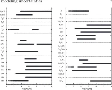
4.1. Results for L134N
Figure 8 shows the times of agreement for each observed molecule towards L134N. With our standard uncertainty of a factor of three in the observed abundances, Model 2 reproduces up to roughly 80% of the 41 observed molecu-les in the range of times (6.0 − 6.8) × 104yr and the level
of agreement tapers off gradually at both younger and
NH3 log [t(yr)] CH2CN C2H2O C3H2 C4H HCOOH HC3N CH3CN CH3OH CH3CHO C2H3CN C3H4 HC5N HC7N HCO+ HCS+ N2H+ H2CN+ H2O O2 C CH CN CO CS NO OH SO C2H C2S H2S HCN HNC OCS SO2 C3H C3N C3O C3S H2CO H2CS log [t(yr)]
Fig. 8. Agreement between the observed abundances to-wards L134N “N” peak) and the predictions of the chem-ical model (Model 2) as a function of time. Symbols in-dicate an agreement between the observational constraint and the model results. Stars are for the observed abun-dances whereas dots and diamonds are for the observa-tional upper and lower limits respectively.
older ages. The peak number increases to 87% if an error of a factor of 5 is taken for the observed values. Model 1 reproduces fewer species (73%), and the best agreement occurs later, at 5 × 10⁵ yr (see Table 5). With Model 2,
the molecules H2S, OCS, CH3OH, CH3CHO are
under-estimated at all times. On the other hand, the observed abundances of HNC, C3H, C3O and NH3 are reproduced
by the model but not at the best range of ages. The three species C3H, HNC, and NH3are in agreement with
obser-vation for times very close to the best range, while C3O
has not been detected and only an upper limit is known. The special cases of O2 and H2O, for which upper limits
have been well studied, are discussed in Sect. 5.1.
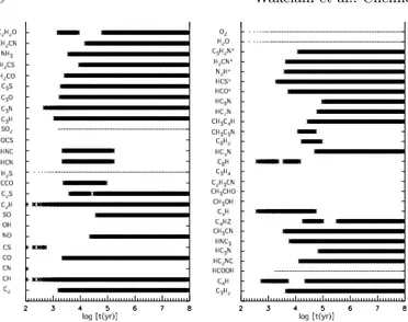
4.2. Results for TMC-1
Using Model 2, we can only reproduce at best 50% of the observed 52 molecular abundances in the CP peak of TMC-1. This percentage is even lower than the 67% ob-tained by Smith et al. (2004), who compared the results of the osu.2003 database with the same observations towards TMC-1CP. These authors considered the modeling to be successful if the differences between the observed and the-oretical values are less than a factor of 10. Smith et al. (2004), Terzieva & Herbst (1998) and Roberts & Herbst (2002) showed that by increasing the C/O elemental ratio, they were able to better reproduce the observations. We then ran a third model (Model 3, see Table 1) identical with Model 2 except that the initial abundance of O is lowered to 1.2 × 10⁻⁴, so that the elemental C/O ratio
becomes 1.2. Fig. 9 shows the comparison with Model 3. Here, seventy-six percent of the molecules are reproduced
Fig. 9. Agreement between the observed abundances to-wards TMC-1 (“CP” peak) and the predictions of the chemical model (Model 3) as a function of time.
considering an observed uncertainty of a factor of 3 at a time of 8 × 10⁴ yr. This number is increased to 86% at
the same age for an observed uncertainty of a factor of 5. The molecules OH, OCS, CH3OH, CH3CHO, C2H3CN
and C3H4are never reproduced by the model whereas the
CN, CS, C5H, HC9N, C6H and CH3C3N abundances are
not reproduced in the optimum age range. The observed abundance of OH in TMC-1 is quite uncertain since it was detected using a significantly larger beam than for the other species, and contamination from other regions of the cloud is probable (Ohishi et al. 1992).
Looking at both clouds, we see that the abundance of the molecules OCS, CH3OH and CH3CHO are
under-estimated at all times by the model compared with the observed values. One explanation could be these species are formed on the grains and released in the gas phase by non-thermal processes (Markwick et al. 2000). Indeed, OCS and CH3OH are known to be present on the grain
mantles with an abundance (comparable to that of H2) of
∼ 10−7 for OCS (Palumbo et al. 1997) and ∼ 10−6 for
CH3OH (Chiar et al. 1996). Work in progress by Garrod
et al. (submitted) with a gas-grain model and various non-thermal desorption mechanisms supports this view. The fact that H2S and NH3 are not reproduced correctly in
L134N may have the same origin since H-enriched mo-lecules are believed to form efficiently on grains although solid H2S has never been detected on grains (van Dishoeck
& Blake 1998). For H-poor species such as CS, CN and HNC, some of the rate coefficients of the critical reac-tions forming and depleting them may be more uncertain than we have assumed, especially if the reactions have not been studied and the estimated uncertainties are hiding non-random errors.
For the case of the two cold cores studied using osu.2003, as opposed to our previous study of hot cores, we find that with our sensitivity technique it is most
of-ten difficult to isolate small numbers of very important reactions for those molecules with abundances we cannot reproduce. Rather, the general picture is that for many species, there are large numbers of reactions that are of relatively equal importance.
There are some reactions deemed important by our sensitivity technique that are critical for all the species: these are the ionization of H2 and He by cosmic
rays, as already noticed by Vasyunin et al. (2004)and Wakelam et al. (2005), and raised in an oral presenta-tion by A. Markwick-Kemper in the 16th UCL Astronomy Colloquium (Windsor, UK, 2002). Ionization reactions in-volving cosmic rays, both direct and indirect, are, how-ever, better thought of as variable parameters rather than reactions with uncertain rates since it not in general the physics of the process but the flux of cosmic rays that is in doubt.
4.3. RATE99 calculations
Before definitively ascribing the disagreements to specific causes, it is useful to see how the comparison with ob-servations is affected by the use of the RATE99 network. Table 5 lists the overall level of agreement for both net-works. On balance, the results with RATE99 show slightly better agreement with observation and show it at later times. Unlike the osu.2003 results, the RATE99 results are in agreement for the saturated species methanol and, in some cases, acetaldehyde. Although this agreement would appear to weaken our argument that the saturated species are produced on grain surfaces, it should be noted that the methanol prediction of RATE99 is almost certainly wrong because the gas-phase synthesis of methanol used:
CH+3 + H2O −→ CH3OH+2 + hν, (2)
CH3OH+2 + e−−→ CH3OH + H, (3)
is assumed to be far too efficient for at least three rea-sons: (i) the radiative association reaction to produce the precursor ion CH3OH+2 has been measured to occur much
more slowly than predicted (Lucas et al. 2002), (ii) the dissociative recombination of this ion leads to methanol in only 6% of collisions (Geppert et al. 2006), and (iii) the water abundance used in the radiative association re-action is far greater than its measured upper limit. New calculations using the RATE99 network now agree with the osu.2003 result that this species cannot be produced in the gas (Geppert et al. 2006).
The case of acetaldehyde may or may not be similar. This species is also thought to be produced via a radiative association
H3O++ C2H2−→ CH3CHOH++ hν, (4)
followed by a dissociative recombination (Herbst 1987):
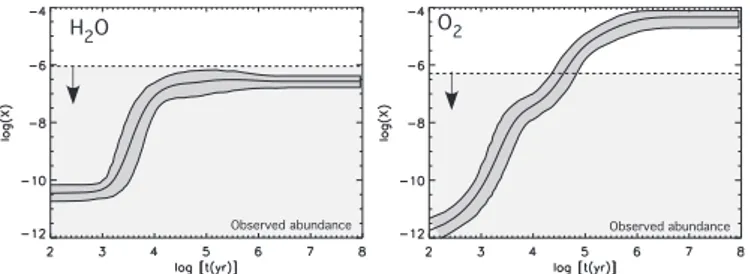
Observed abundance H2O
Observed abundance
O2
Fig. 10.Comparison between the theoretical abundances with error bars of H2O and O2 (Model 2) and the upper
limits of the abundances found in L134N (see Table 4)
There is no direct evidence for either reaction, although the association does occur at high densities in the labora-tory via collisional stabilization (Herbst 1987).
We conclude that there is substantial evidence that methanol is only produced on grains, although the case against gas-phase production of acetaldehyde is not quite proven. It is likely though that the high abundance of acetaldehyde in the RATE99 calculation stems at least partially from an overly slow destruction by ions since this species has a dipole moment. The percentages of species in agreement using the RATE99 database listed in Table 5 do not include the agreement with these two species.
5. Discussion
5.1. Special cases of water and molecular oxygen
An interesting result of this work is that it provides an-other manner in which the low upper limits to the abun-dances of gas-phase H2O and O2 in cold cores, detected
by the SWAS and Odin satellites, can be explained (Snell et al. 2000; Pagani et al. 2003). Essentially, the upper limit of the observed abundance (multiplied by a factor of three given our standard chosen observational uncer-tainties) must not be less than the lower error bar of the theoretical abundance.
Let us first consider the case of L134N. In Fig. 10, we plot the calculated Model 2 abundances for water and oxygen with error bars as functions of time and superim-pose the measured upper limits multiplied by a factor of three. The results show that both species are successfully reproduced in the optimum age range defined by the max-imum agreement with all species, although the case of O2
is much more marginal since it is clearly overproduced at times after 105yr. This result shows that interaction with
grain surfaces is not necessarily required if we consider young clouds (≤ 105yr). The abundance of O
2was found,
however, to be lower than the value for L134N (< 10−7)
in a dozen dark clouds (Pagani et al. 2003), which we ex-pect to have different ages. It may then be necessary to invoke depletion processes to explain the low abundance of O2in quiescent cores (see Roberts & Herbst 2002). The
case of TMC-1 is singular since we used a model (Model 3) with high elemental C/O ratio. Here there are no age constraints (see results in Fig. 9).
TMC-1 L134N Distance of disagreement D [ log( X) ]
Fraction of reproduced molecules
TMC-1 L134N F log(t[yr]) ( mi n (D )/D )*F TMC-1 L134N
Fig. 11. Upper panel: the fraction of molecules repro-duced by the model as a function of time for both clouds (Model 2 for L134N and Model 3 for TMC-1). Middle panel: the distance D of disagreement between the ob-served and modeled abundances (see text for details). Lower panel: the fraction of reproduced molecules multi-plied by min(D)/D (minimum of the distance of disagree-ment divided by the distance of disagreedisagree-ment). We con-sider a factor of 3 uncertainty in the observed abundances.
5.2. Age of the clouds: a more refined estimate
Our models of quiescent cores are clearly not the com-plete picture since dynamical forces are producing and destroying cores while chemistry occurs (Garrod et al. 2005). For TMC-1 and L134N, the creation and chemistry have been occurring to some extent simultaneously. So, our pseudo-time-dependent calculations represent a crude approximation, with frankly an uncertain zero-time condi-tion. Even within this crude approximation, we have used a less than perfect criterion to determine the “chemical” age for TMC-1CP and L134N by simply maximizing the number of molecules with calculated abundances and er-ror bars in agreement with observed values. Essentially, we have made no allowance for the quality of the agree-ment and the extent of the disagreeagree-ment for individual species. The results of this simple method are re-plotted in the top panel of Fig. 11 for L134N (Model 2) and TMC-1CP (Model 3) as the fraction F of molecules in agreement vs time. In this representation, we can see that the best age for L134N is somewhat more distinct that for TMC-1CP, but that the optimum ages lie in what previously was known as “early time”, well before steady-state conditions set in.
To do somewhat better, we first compute an arbitrary parameter called the distance of disagreement D, which is defined, for the species not reproduced by the model, as the sum over all species of the distance di (in units of
log X, see Fig. 7) between the observational value and the theoretical one. For example, if for a particular species, i, Xobs> Xmodel then the contribution to D is given by the
expression
di= log Xobs;min− log Xmodel;max, (6)
where the maximum and minimum values refer to the er-ror bars. The middle panel of Fig. 11 shows the total dis-tance D as a function of time for the two clouds. This plot indicates that the disagreement with the model reaches a minimum, labeled min(D), somewhat after 104yr. Finally,
the lower panel of Fig. 11 shows a plot vs time of the ra-tio between the minimum distance, min(D), and D, mul-tiplied by the fraction of reproduced molecules, F. This quantity, which includes the strength of individual dis-agreements for specific species, tends to sharpen the best age, especially for L134N. In particular, we obtain a sharp maximum for L134N around 6 × 10⁴yr and a less marked
maximum for TMC-1CP around 105 yr. These numbers
are not strikingly different from a variety of other esti-mates, but must be taken with extreme caution. The ages derived analogously with the RATE99 set of reactions are somewhat larger, ∼ 106 yr.
6. Conclusions
In this paper, we have reported the use of our Monte Carlo approach to uncertainties in calculated abundances to study the gas-phase chemistry of dark clouds, in partic-ular the well-studied sources TMC-1CP and L134N. We have utilized models in which the uncertainties in both rate coefficients and physical conditions are included; the latter can be thought of as either the actual observational uncertainties or physical heterogeneities in the sources. With a specific criterion for agreement between observa-tion and theory in which the errors in both techniques must overlap, we find that most but not species detected in the sources are reasonably well accounted for at so-called “early time,” a far from novel result although one determined more rigorously than in previous approaches. A major goal of the study has been to gain some in-sight as to which failing of the simple picture utilized is the more important: the lack of grain-surface chemistry or the lack of a dynamical model of the sources. For sat-urated (H-rich) species, with reasonably understood syn-theses on grain surfaces, our results support earlier indi-cations that surface chemistry is an important, probably a critical omission, but for unsaturated species, the picture remains less clear because it is difficult to determine from our sensitivity analysis whether the discrepancies can be accounted for by poorly determined rates of critical chem-ical reactions. This difficulty stems from the fact that the chemistry of unsaturated species often seems to involve
contributions from large numbers of poorly determined reaction rates.
The fact that discrepancies for the calculated abun-dances of individual species between two chemical works used, our osu.2003 network and the RATE99 net-work, can be larger than their calculated random uncer-tainties indicates that more attention must be paid in the laboratory to specific classes of reactions, such as ion-polar neutral systems, before more definitive conclusions can be reached. Further complicating the issue are other concerns such as the proper initial make-up of the gas, what elemental abundances are reasonable, and the range over which the cosmic ray ionization rate ζ can be varied. Nevertheless, our study indicates strongly that gas-phase models of static sources cannot represent the complete picture. More complex treatments, involving cycles of sur-face adsorption, reaction, and desorption, possibly coupled with dynamical histories of the sources, would appear to be required.
Acknowledgements. We thank the National Science Foundation for its support of the astrochemistry program at Ohio State.
References
Chiar, J. E., Adamson, A. J., & Whittet, D. C. B. 1996, ApJ, 472, 665
Dickens, J. E., Irvine, W. M., Snell, R. L., et al. 2000, ApJ, 542, 870
Garrod, R., Park, I.-H., Caselli, P., & Herbst, E. submit-ted, Disc. Faraday Soc.
Garrod, R. T., Williams, D. A., Hartquist, T. W., Rawlings, J. M. C., & Viti, S. 2005, MNRAS, 356, 654 Geppert, W. D., Hellberg, F., & Osterdahl, F. e. a. 2006, in in Astrochemistry Throughout the Universe: Recent Successes and Current Challenges (IAU Symposium 231), eds. Lis, D. C., Blake, G. A. and Herbst, E. (Cambridge Univ. Press), in press
Hartquist, T. W., Williams, D. A., & Viti, S. 2001, A&A, 369, 605
Hasegawa, T. I., Herbst, E., & Leung, C. M. 1992, ApJS, 82, 167
Herbst, E. 1987, ApJ, 313, 867
Herbst, E. & Klemperer, W. 1973, ApJ, 185, 505 Herbst, E. & Leung, C. M. 1986, ApJ, 310, 378
Langer, W. D., Graedel, T. E., Frerking, M. A., & Armentrout, P. B. 1984, ApJ, 277, 581
Le Bourlot, J. 1991, A&A, 242, 235
Le Teuff, Y. H., Millar, T. J., & Markwick, A. J. 2000, A&AS, 146, 157
Leung, C. M., Herbst, E., & Huebner, W. F. 1984, ApJS, 56, 231
Lucas, A., Voulot, D., & Gerlich, D. 2002, in WDS’02 (Prague) Proceedings of Contributed Papers, PART II, 294
Markwick, A. J., Millar, T. J., & Charnley, S. B. 2000, ApJ, 535, 256
Millar, T. J. & Nejad, L. A. M. 1985, MNRAS, 217, 507 Neufeld, D. A., Wolfire, M. G., & Schilke, P. 2005, ApJ,
628, 260
Nomura, H. & Millar, T. J. 2004, A&A, 414, 409
Ohishi, M., Irvine, W. M., & Kaifu, N. 1992, in IAU Symp. 150: Astrochemistry of Cosmic Phenomena, Vol. 150, 171
Pagani, L., Olofsson, A. O. H., Bergman, P., et al. 2003, A&A, 402, L77
Palumbo, M. E., Geballe, T. R., & Tielens, A. G. G. M. 1997, ApJ, 479, 839
Prasad, S. S. & Huntress, W. T. 1980, ApJS, 43, 1 Pratap, P., Dickens, J. E., Snell, R. L., et al. 1997, ApJ,
486, 862
Roberts, H. & Herbst, E. 2002, A&A, 395, 233
Rowe, B. R. 1992, in IAU Symp. 150: Astrochemistry of Cosmic Phenomena, 7
Rowe, B. R. & Rebrion, C. 1992, Trends in Chem. Phys., 1, 367
Ruffle, D. P. & Herbst, E. 2000, MNRAS, 319, 837 Smith, I. W. M., Herbst, E., & Chang, Q. 2004, MNRAS,
350, 323
Snell, R. L., Howe, J. E., Ashby, M. L. N., et al. 2000, ApJ, 539, L101
Stark, R., Wesselius, P. R., van Dishoeck, E. F., & Laureijs, R. J. 1996, A&A, 311, 282
Su, T. & Chesnavich, W. J. 1982, J. Chem. Phys., 76, 5183 Terzieva, R. & Herbst, E. 1998, ApJ, 501, 207
van Dishoeck, E. F. & Blake, G. A. 1998, ARA&A, 36, 317
Vasyunin, A. I., Sobolev, A. M., Wiebe, D. S., & Semenov, D. A. 2004, Astronomy Letters, 30, 566
Wakelam, V., Selsis, F., Herbst, E., & Caselli, P. 2005, A&A, 444, 883