HAL Id: hal-00317029
https://hal.archives-ouvertes.fr/hal-00317029
Submitted on 1 Jan 2003
HAL is a multi-disciplinary open access
archive for the deposit and dissemination of
sci-entific research documents, whether they are
pub-lished or not. The documents may come from
teaching and research institutions in France or
abroad, or from public or private research centers.
L’archive ouverte pluridisciplinaire HAL, est
destinée au dépôt et à la diffusion de documents
scientifiques de niveau recherche, publiés ou non,
émanant des établissements d’enseignement et de
recherche français ou étrangers, des laboratoires
publics ou privés.
stratospheric potential vorticity fields
R. Huth, P. O. Canziani
To cite this version:
R. Huth, P. O. Canziani. Classification of hemispheric monthly mean stratospheric potential vorticity
fields. Annales Geophysicae, European Geosciences Union, 2003, 21 (3), pp.805-817. �hal-00317029�
Geophysicae
Classification of hemispheric monthly mean stratospheric potential
vorticity fields
R. Huth1and P. O. Canziani2,3
1Institute of Atmospheric Physics, Praha, Czech Republic
2Grupo de Atm´osfera Media, Departamento de Ciencias de la Atm´osfera y los Oc´eanos, Facultad de Ciencias Exactas y Naturales, CONICET/Universidad de Buenos Aires, Buenos Aires, Argentina
3Unidad Docente Ciencias B´asicas Matem´atica, Facultad Regional Buenos Aires, Universidad Tecnol´ogica Nacional, Argentina
Received: 11 March 2002 – Revised: 21 August 2002 – Accepted: 20 September 2002
Abstract. Monthly mean NCEP reanalysis potential vortic-ity fields at the 650 K isentropic level over the Northern and Southern Hemispheres between 1979 and 1997 were studied using multivariate analysis tools. Principal component anal-ysis in the T-mode was applied to demonstrate the validity of such statistical techniques for the study of stratospheric dynamics and climatology. The method, complementarily applied to both the raw and anomaly fields, was useful in de-termining and classifying the characteristics of winter and summer PV fields on both hemispheres, in particular, the well-known differences in the behaviour and persistence of the polar vortices. It was possible to identify such features as sudden warming events in the Northern Hemisphere and final warming dates in both hemispheres. The stratospheric im-pact of other atmospheric processes, such as volcanic erup-tions, also identified though the results, must be viewed at this stage as tentative. An interesting change in behaviour around 1990 was detected over both hemispheres.
Key words. Meteorology and atmospheric dynamics (mid-dle atmosphere dynamics; general circulation; climatology)
1 Introduction
Multivariate statistical methods have evolved as useful tools in analysing large-scale features of tropospheric circulation and temperature. They allow, among other things, the iden-tification of (i) modes of variability, frequently referred to as teleconnections in the tropospheric context (e.g. Barn-ston and Livezey, 1987); (ii) preferred circulation regimes and recurrent circulation patterns (Toth, 1993; Michelangeli et al., 1995), and (iii) relationships between two fields, for example, sea surface temperature and geopotential heights (Bretherton et al., 1992). In the stratosphere, however, the applications of multivariate statistical methods have been so far rather scarce. The reason for that probably lies in a Correspondence to: P. O. Canziani
comparative simplicity of stratospheric fields with respect to tropospheric ones. Nevertheless, there are a number of studies that have successfully employed multivariate meth-ods in stratospheric analyses. For example, Perlwitz and Graf (1995) applied principal component analysis to identify three modes of variability in the Northern Hemisphere win-ter monthly mean 50 hPa geopotential heights, and canonical correlation analysis, to find couplings between stratospheric and tropospheric circulation. For the latter purpose, Cheng and Dunkerton (1995) used rotated singular value decompo-sition analysis. Eder et al. (1999) studied daily total ozone data with PCA, which resulted in the regionalisation of the globe, according to the temporal behaviour of ozone. Con-cerning classification studies, Pierce and Fairlie (1993) iden-tified three preferred flow regimes in the 10 hPa heights in the Northern Hemisphere winter. More recently, Compag-nucci et al. (2001) and Salles et al. (2001) carried out a de-tailed analysis of monthly mean lower stratospheric temper-ature anomalies from the MSU retrievals, in order to study its temporal and spatial variability over the Southern Hemi-sphere.
The purpose of this paper is to introduce the classifica-tion method based on the PCA in a T-mode into strato-spheric research, to use it for identification of typical (re-current) monthly mean potential vorticity patterns on both hemispheres, and to illustrate its benefits, mainly in detect-ing/typifying various features of stratospheric circulation and dynamics. A brief overview of the methodology used here is given in Sect. 2. The data set is described in Sect. 3 and the results discussed in Sect. 4.
2 Classification method
Several classification methods have found their application in the atmospheric sciences. They include correlation-based methods, cluster analysis and principal component analysis (PCA). For a review, refer to Huth (1996a). We decided to
Fig. 1. Eigenvalue vs. PC number plot for raw data for Northern
Hemisphere (NH) and Southern Hemisphere (SH).
use PCA in this study for its good stability and ability to uncover the underlying structure of data (Huth 1996a).
A brief description of PCA follows; further details may be found in the review paper by Richman (1986), and references therein. PCA consists of expressing a data matrix Z= (zij), i = 1, ..., N indexing observations (realisations, cases) and j = 1, ..., n indexing variables (individuals), as a product Z = FAT. Here, F = (fim) and A = (ajm)are matrices of principal component (PC) scores (amplitudes) and loadings, respectively. The loadings are eigenvectors of a data simi-larity matrix (correlation and covariance are most frequently used as a similarity measure) scaled by the square root of the corresponding eigenvalue. The eigenvalues equal the vari-ance explained by a particular PC. The system of PCs has two fundamental properties: (a) both the loadings and scores are orthogonal to one another, and (b) the i-th PC maximises the variance unexplained by the first to (i − 1)t hPC. PCs are by convention ordered according to the magnitudes of eigen-values. A few leading PCs usually account for large amounts of total variance, concentrating the physical signal. A num-ber of subsequent PCs may contain information about certain particular conditions, i.e. events with a lower recurrence in the data sample considered, or isolated/exceptional events. Consequently, the matrices of PC loadings and scores may be truncated after relatively few r columns, r <= n, with-out loss of relevant information. The interpretation of PCs may be frequently improved, and their stability enhanced, if they are subject to rotation. The rotation is performed at the expense of losing the maximum variance (orthogonal rota-tions) and orthogonality (oblique rotarota-tions) properties. The use of rotation requires careful inspection of the results to verify whether there has been an actual improvement, i.e. its application should definitely not be considered for automatic or “black-box” use.
The data matrix Z can be specified in several ways, de-pending on which parameters are treated as fixed entities,
variables, and their realisations. These specifications are re-ferred to as modes of decomposition (Richman, 1986). If the field is kept fixed, there are two possibilities of arrang-ing Z: either grid point (or station) values are identified with variables (i.e. columns in Z) and time observations with re-alisations (rows in Z), or vice versa, time observations rep-resent variables and grid points (stations) reprep-resent realisa-tions. The former arrangement is commonly referred to as an S-mode, the latter as a T-mode. Compagnucci and Ruiz (1992), Drosdowsky (1993), Huth (1993, 1997), Compag-nucci et al. (2001) and Salles et al. (2001) contrasted the use of the two modes. Whereas the S-mode isolates groups of grid points (stations) at which the analysed variable varies similarly in time, the T-mode analysis identifies groups of observations (days, months, etc.) with similar spatial pat-terns, for example, fields. Therefore, if the classification of patterns is the goal, PCA must be used in the T-mode. Indi-vidual patterns are classified according to their highest load-ing (in the absolute sense), because the higher the loadload-ing, the better the similarity with the type represented by the PC. Since loadings may attain both positive and negative values, for a particular number of PCs we may potentially obtain twice as many types, sometimes referred to as direct and in-verse, or positive and negative, respectively. Here we adhere to the latter nomenclature. More details of the application of T-mode PCA to classification can be found in Huth (1996b), and Salles et al. (2001).
In the course of the analysis, several methodological ques-tions should be raised and answered:
1. What input data to use: raw data or anomalies? If anomalies (i.e. deviations from long-term mean values or seasonal/annual cycles) are used, only the position of anomaly centres on a map, their intensities are not taken into account. On the other hand, if raw data enter PCA, both position and intensity of features (vortex, ridges, troughs, strong gradients, etc.) are reflected in classifi-cation (Huth 1995, 1996b), i.e. two patterns, one with weak and one with strong anomaly at the same posi-tion, are classified with the same type in anomaly data, but may be classified with different types in raw data. In our study, we examine both raw data and anomalies, and illustrate the effect of this choice on the classifica-tion output.
2. Which similarity matrix to use? For classification of tropospheric circulation, whether correlation or covari-ance matrix is used makes little difference (Huth, 1995). The analysis of MSU lower stratospheric temperature anomalies has shown that the most direct description of real fields is obtained with the correlation matrix (Salles et al., 2001). Therefore, the correlation matrix is used in our study.
3. How many PCs to retain, i.e. how many appropriate types are produced? There are many criteria for de-termining the number of PCs to retain, i.e. to use for interpretation. However, different criteria frequently
Table 1. The occurrence of types in individual months in years 1979
to 1997 (denoted by the last two digits) for 2 rotated PCs of raw data in NH. The summer type (1) is shaded for easier visualization
79 80 81 82 83 84 85 86 87 88 89 90 91 92 93 94 95 96 97 1 2 2 2 2 2 2 1 2 2 2 2 2 2 2 2 2 2 2 2 2 2 2 2 2 2 2 2 2 1 2 2 2 2 2 2 2 2 2 2 3 1 2 1 2 2 1 2 2 1 2 1 2 2 2 2 2 2 2 2 4 1 1 1 1 1 1 1 1 1 1 1 2 1 1 1 1 1 1 2 5 1 1 1 1 1 1 1 1 1 1 1 1 1 1 1 1 1 1 1 6 1 1 1 1 1 1 1 1 1 1 1 1 1 1 1 1 1 1 1 7 1 1 1 1 1 1 1 1 1 1 1 1 1 1 1 1 1 1 1 8 1 1 1 1 1 1 1 1 1 1 1 1 1 1 1 1 1 1 1 9 1 1 1 1 1 1 1 1 1 1 1 1 1 1 1 1 1 1 1 10 2 2 2 2 2 2 2 2 2 2 2 2 2 2 2 2 2 2 2 11 2 2 2 2 2 2 2 2 2 2 2 2 2 2 2 2 2 2 2 12 2 2 2 2 2 2 2 2 1 2 2 2 2 2 2 2 2 2 2
yield disparate results (Richman et al., 1992; Serrano et al., 1999). An eigenvalue (or log-eigenvalue) vs. PC number diagram frequently provides a good guide: it is recommended to cut the number of PCs just after a sec-tion of relatively small slope on the diagram, followed by a pronounced drop (O’Lenic and Livezey, 1988). This secures that a “degenerate multiplet”, which can be formed by PCs with close eigenvalues, is not separated (North et al., 1982). This partly subjective criterion was found to be well applicable if PCA is used for classifica-tion (Huth, 1996b). In our study we examine soluclassifica-tions based on several numbers of components, allowed by that criterion. This introduces some ambiguity into the analysis; we show, nevertheless, that analyses based on different numbers of PCs may complement each other. This means that the ambiguity may, in fact, become ben-eficial.
4. Rotate or not? As stated above, rotation may facilitate a physical interpretation of components. We discuss the effect of rotation later. For rotation, the oblique “Direct Oblimin” procedure was used.
3 Data
We examine monthly mean potential vorticity (PV) fields at the 650 K isentropic level. This corresponds to approx-imately 30 hPa or the altitudes of 22–24 km. In the polar region this is a height where the interior of the winter po-lar vortex, whose areal extent is commonly given by the area enclosed within the strongest high latitude PV gradients, is usually well isolated from mid-latitudes. Hence, little mixing between the inner ozone poor air and the outer ozone-rich air takes place, thus effectively confining the low ozone region (Chen et al., 1994). Given that the winter polar vortex repre-sents the largest possible areal extent for the ozone depletion region, the study of the PV field also provides insights into the dynamic behaviour of the ozone hole. Inspection of PV plots between 400 K and 650 K shows that, in general, the vortex edge is fairly well aligned in that height range (e.g. Waugh and Randel, 1999), and even more so in the monthly
Fig. 2. Composite mean PV patterns (in PV units) for the NH types
based on 2 rotated PCs of raw data. The outer circle is 20◦N; the Greenwich meridian points to the left, 90◦E downward, etc. Each type is identified by the number of corresponding PCs; its total fre-quency is given in parentheses.
Fig. 3. Similar as in Fig. 2 except for the SH types. The outer
circle in the maps is 20◦S; the Greenwich meridian points to the left, 90◦E upward, etc.
mean values considered here. Hence, this allows the compar-ison between the present analysis and similar analysis car-ried out for MSU Ch4 temperature, which corresponds to the 100–50 hPa region. According to the hydrostatic approxima-tion, geopotential height anomalies, and thus resulting PV anomalies in a layer reflect the temperatures below.
Both hemispheres are analysed separately. The monthly mean fields were taken poleward of 20◦. The analysis
cov-ers a 19-year period from 1979 to 1997. This period was chosen to coincide with the MSU anomaly data available, which was analysed in Compagnucci et al. (2001) and Salles et al. (2001), so that possible comparisons between the lower stratospheric temperature field and PV may be statistically sound. The tropical region is not considered here, given the current limitations of such a highly derived variable in that region of the atmosphere. The source of data are the NCEP reanalyses products (Kalnay et al., 1996), reduced to a 5◦ latitude by 10◦longitude grid.
Table 2. As in Table 1 except for SH; the summer type (2) is shaded 79 80 81 82 83 84 85 86 87 88 89 90 91 92 93 94 95 96 97 1 2 2 2 2 2 2 2 2 2 2 2 2 2 2 2 2 2 2 2 2 2 2 2 2 2 2 2 2 2 2 2 2 2 2 2 2 2 2 2 3 2 2 2 2 1 2 1 2 2 2 2 2 2 2 2 2 1 2 2 4 1 1 1 1 1 1 1 1 1 1 1 1 1 1 1 1 1 1 1 5 1 1 1 1 1 1 1 1 1 1 1 1 1 1 1 1 1 1 1 6 1 1 1 1 1 1 1 1 1 1 1 1 1 1 1 1 1 1 1 7 1 1 1 1 1 1 1 1 1 1 1 1 1 1 1 1 1 1 1 8 1 1 1 1 1 1 1 1 1 1 1 1 1 1 1 1 1 1 1 9 1 1 1 1 1 1 1 1 1 1 1 1 1 1 1 1 1 1 1 10 1 1 1 1 1 1 1 1 1 1 1 1 1 1 1 1 1 1 1 11 2 1 1 1 1 1 1 2 1 2 1 1 2 1 1 1 1 1 1 12 2 2 2 2 2 2 2 2 2 2 2 2 2 2 2 2 2 2 2 4 Results 4.1 Raw data
In the analysis of raw data, the first PC is clearly dominant, explaining about 85% of total variance in both hemispheres (Fig. 1). This is a common output if PCA in a T-mode is applied to raw data; the first unrotated PC may be interpreted as the time mean pattern (Huth, 1996b), provided it is the most frequent physical field during the period sampled. As a result of such a dominance, unrotated loadings of the first PC are far higher than those obtained for subsequent PCs. The classification (in the usual sense, i.e. assignment of each pattern to a single class or type), based on unrotated loadings, is, therefore, not possible, although individual PCs may be interpreted (Compagnucci and Salles, 1997).
The classification may be achieved through the use of ro-tation. The eigenvalue vs. PC number diagram (Fig. 1) does not display a clear drop from signal to noise for either hemi-sphere. There are, however, suggestions of preference for several numbers of PCs to rotate. We decided to perform rotation for all the numbers of PCs from 2 to 10 for both hemispheres; this can provide us with an idea on the sta-bility of solutions. It is worth noting that no negative load-ing appeared in any solution as the largest in the absolute sense. Therefore, only positive types (corresponding to pos-itive loadings) occur, so the number of types is equal to the number of rotated PCs.
4.1.1 Two principal component analyses
First let us discuss the solution for two rotated PCs, i.e. the classification with two types. Figures 2 and 3 display the composite mean patterns for the two types in the Northern and Southern Hemisphere, respectively. Tables 1 and 2 show which types the individual monthly patterns are assigned to. The classification clearly distinguishes between a strong po-lar vortex with steep gradients around 65◦, somewhat shifted towards Eurasia, and a more homogeneous field without vor-tex features, prevailing in the winter and summer periods, respectively. The occurrence of the NH winter type is con-fined from October until March, with a couple of additional occurrences in April. The NH summer type occurs in April to September, and occasionally also appears in the winter
Table 3. As in Table 1 but for 8 rotated PCs of raw data. The
summer type (1) is shaded
79 80 81 82 83 84 85 86 87 88 89 90 91 92 93 94 95 96 97 1 2 8 2 3 2 2 3 2 2 1 8 2 5 2 8 2 2 5 5 2 4 2 3 5 2 2 7 2 6 8 5 4 2 2 2 5 4 2 5 3 1 2 4 5 3 1 4 4 1 7 1 7 2 4 5 7 5 2 8 4 1 1 1 4 1 1 1 1 1 1 1 1 1 1 1 1 1 1 7 5 1 1 1 1 1 1 1 1 1 1 1 1 1 1 1 1 1 1 1 6 1 1 1 1 1 1 1 1 1 1 1 1 1 1 1 1 1 1 1 7 1 1 1 1 1 1 1 1 1 1 1 1 1 1 1 1 1 1 1 8 1 1 1 1 1 1 1 1 1 1 1 1 1 1 1 1 1 1 1 9 1 1 1 1 1 1 1 1 1 1 1 1 1 1 1 1 1 1 1 10 1 1 1 1 1 1 1 1 1 1 1 1 1 1 1 1 1 1 1 11 4 1 2 8 7 4 5 5 2 8 4 8 8 2 5 4 2 2 8 12 1 8 4 2 2 5 5 8 3 8 8 8 8 5 2 8 8 4 2
Table 4. As in Table 3 but for SH. In dark and light shading are the
summer type (2) and the transition types (3 to 8), respectively
79 80 81 82 83 84 85 86 87 88 89 90 91 92 93 94 95 96 97 1 2 2 2 2 2 2 2 2 2 2 2 2 2 2 2 2 2 2 2 2 2 2 2 2 2 2 2 2 2 2 2 2 2 2 2 2 2 2 2 3 2 2 2 2 2 2 2 2 2 2 2 2 2 2 2 2 2 2 2 4 2 2 2 4 2 2 4 2 2 2 2 4 2 2 2 2 4 2 5 5 1 4 1 4 4 7 4 7 4 4 4 7 1 7 4 7 4 4 7 6 1 4 1 1 1 1 1 1 1 1 1 1 1 8 1 8 1 8 1 7 1 1 1 1 1 1 1 1 1 1 1 1 1 1 1 1 1 1 1 8 1 1 1 1 1 1 1 1 1 8 1 1 1 1 1 1 1 1 1 9 1 1 1 1 1 1 1 1 1 8 1 1 3 1 8 1 8 8 7 10 8 3 8 5 5 3 5 7 1 3 8 1 3 5 7 8 5 5 5 11 2 3 3 7 2 5 5 5 4 2 5 4 5 5 3 3 3 3 7 12 2 2 2 2 2 2 2 2 2 2 2 2 2 2 2 2 2 2 2
months, i.e. January 1985 and December 1997. In SH, win-ter types occur from April to October, summer types from December to February, with March and November being the transition months. In contrast to NH, no summer types occur within the winter period and vice versa. The mean position of the winter vortex appears to be shifted towards the Green-wich meridian and South Atlantic. Such a clear-cut result with two types for each hemisphere reflects the well-known behaviour of the polar vortex. Indeed, the NH polar vortex is a distinct winter feature, with a sizeable amount of intrasea-sonal variability, due to sudden warming and wave events, as will be discussed subsequently. It is interesting to note that the polar vortex pattern, for all the years considered here, be-comes established during October, but can break up any time between March and May. The SH polar vortex is a much stronger phenomenon with a limited variability and it lasts well into spring, i.e. it is much longer lived. Furthermore, November appears as a transition month, since the polar vor-tex has extended its life span into this month over the years sampled. The years where the SH polar vortex pattern only lasts through October are coincident with years of early dis-appearance of the ozone hole, for example, 1988. This is to be expected, since the ozone hole’s life cycle is dependent, during each annual event, on the evolution of the polar vor-tex.
Fig. 4. As in Fig. 2 except for 8 rotated PCs of raw data.
4.1.2 Eight principal component analyses
If the number of rotated PCs (and hence, the number of types) is increased, the types with no vortex (summer types) remain almost unchanged, whereas the winter types are split into more classes differing in the position, intensity and asymme-try of the polar vortex. This is reasonable, since the summer stratosphere does not exhibit any dominant features, i.e. the planetary wave activity and hence, variability is very limited. The classifications for eight PCs are presented in Figs. 4 and 5, and Tables 3 and 4.
The NH polar vortex tends to be located over Eurasia or the Arctic region, in agreement with ozone loss observations by TOMS (Total Ozone Mapping Spectrometer), GOME (Global Ozone Monitoring Experiment) and UARS (Upper Atmosphere Research Satellite) ozone observations. While
Fig. 5. As in Fig. 3 except for 8 rotated PCs of raw data.
only PC5 and PC8 show the polar vortex located over the North Pole, the remaining PC’s show the variability in its location over the North Atlantic and Eurasia. PC8, with a very sharp PV gradient, appears primarily during the months of November, December and January, i.e. it corresponds to a strong stable vortex unaffected by mid-latitude wave activity. PC5 corresponds to a vortex with a slightly weaker PV gra-dient, with a more elongated shape. Though also appearing during core winter months, this mode can occur throughout the vortex season. It must be noted that though there were a few isolated occurrences of these two modes in the early 1980s, their recurrence was enhanced starting in 1988–1989. PC8 was particularly recurrent during the early 1990s. Note that in the previous cases (Table 1), when winter months were typified by a summer mode, the present analysis yields PC4,
PC3, or PC6, all of which correspond to rather weak vortex structures. PC3 only appears up to 1987 and PC6 only once during February 1987. During the first 10 years of the sam-ple, the most frequent type during the last month in the polar vortex life cycle was PC4, showing a weak polar vortex at 90◦E over Central Asia. During this period, the final winter month could occur anywhere between February and April. During subsequent years, there appears to be a larger vari-ability in the shape and location of the polar vortex during this stage, together with a sustained presence at least through March. This suggests a more persistent and colder vortex, with more frequently recurrent polar centred modes in later years, together with a larger interannual variability in the NH mid- to high-latitude circulation. Such results agree with ob-servations of deepening Arctic ozone depletion events.
In SH, there is no monthly pattern for which the loading of PC 6 is highest, so no month is classified with the corre-sponding type. On the other hand, PC1, in which the vor-tex is almost perfectly centred over the South Pole, clearly dominates the core months in the vortex life cycle. Until 1988 this pattern prevailed through September. However, since that year there has been a significant interannual vari-ability, even during this month. The initial vortex is most frequently typified by PC4. Though present throughout the sample, this mode occurred more regularly during the late 1980s and early 1990s. Following the PC1 core period, the most frequent types are PC3 and PC8, which describe a vor-tex displaced towards South America and the South Atlantic. PC8 shows a particularly strong PV gradient on the vortex edge. Both have become much more frequent in the 1990s. Occasionally, during the latter stages in the SH polar vor-tex evolution, the vorvor-tex is shifted towards Africa (PC7) or the eastern Indian Ocean (PC5). PC5 occurred throughout the sample, though there are a couple of sequences at least 2 years long when it did not appear. Again, PC7 mode also occurs all along the sample but has become more common in later years. There is no distinct change over the years in the evolution of the final stages of the vortex, though PC3 appears to have dominated during the 1990s.
There is a notable difference between the hemispheres. While most NH winter types occur without any obvious pref-erence for any particular month, the SH types tend to occur at preferred times. Furthermore, there is little interannual variability in the SH, in contrast to the NH. The reason for such a difference lies in that the shape and strength of the polar vortex are subject to a large interannual variability in the NH, due to circulation pattern variability in the tropo-sphere, as well as interannual variability in the occurrence and strength of sudden warmings, as discussed in the next subsection. In the SH, on the other hand, the impact of the interannual variability is not as significant at high latitudes, since the polar vortex is much stronger and continues to grow into the early spring. Furthermore, planetary wave activity is more limited over the SH. There is usually a final warming only, with no major sudden warmings. The evolution of the SH dynamics is much closer to radiative equilibrium. Thus, the annual cycle is the main factor in its evolution. Indeed,
the SH polar vortex, in agreement with the sequence of PCs mentioned above, tends to spend the winter months centred over the South Pole. Then, in spring it starts to have a prefer-ential location towards the eastern South Pacific, then south-ern South America and finally the South Atlantic, after which it breaks up. The present results show that this evolution has become more common during the 1990s. Such behaviour can be detected in the TOMS total ozone retrievals as well. 4.1.3 Seasonal transitions, sudden and final warming
events
Let us now compare the two classifications in more detail. October in NH and April in SH are assigned to the winter type in the 2 PC solution, but to the summer type in the 8 PC solution. The loadings of the two PC solutions for both NH October and SH April patterns tend to be relatively low (about 0.5) and close to each other, indicating that the individual monthly patterns do not greatly resemble either of the types. Nevertheless, the similarity of the real fields with the winter pattern with a strong vortex (which approx-imately represents winter mean conditions) is slightly more pronounced. In the 8 PC solution, more specific patterns are identified as winter types, which leads to their dissimilarity from the winter mean and consequently, the NH October and SH April monthly patterns can be better identified as summer or transition patterns in the latter analysis.
During the NH winter months, the PV patterns are classi-fied with the summer type for the two PC solutions in January 1985, February 1987, and December 1987 (cf. Table 1). All of these months exhibit major mid-winter warmings (Bald-win and Dunkerton, 1989; Erlebach et al., 1996; Fairlie and O’Neill, 1988), which is manifested in a considerably weak-ened polar vortex. In the eight PC solutions, the three months are classified with types 3 or 6 (Table 3), both having indeed a relatively weak vortex, displaced equatorward over the Eu-ropean or Asian sectors. Baldwin and Dunkerton (1989) showed this to be the location of the PV centre at 600 K on individual daily maps following the onset of the 1987/1988 warming. In the eight PC analyses summer type PC1 oc-curs in the winter months of December 1979 and January 1988. The latter is a continuation of the early 1987/1988 ma-jor warming. There are, however, mama-jor warming events that are not detected as summer types nor “major warming” types (3 and 6 in the eight PC classifications), e.g. the warming of January 1991 (Labitzke and van Loon, 1999). The likely reason lies in the monthly averaging interval, which may be too long to catch processes evolving on shorter time scales, such as major warming onsets and breakdowns. Thus, let us consider the stratospheric warmings classification by Lab-itzke and Naujokat (2000), which is based on the FUB (Freie Universitat Berlin) analysis monthly mean temperatures at 30 hPa over the North Pole. The authors consider Canadian, major mid-winter and minor warmings. When using their classification, the following results are obtained:
2. PC2 – four events: Jan. 1986, Feb. 1991, Dec. 1993, and Nov. 1996;
3. PC3 – three events: Feb. 1981, Jan. 1985, and Dec. 1987;
4. PC4 – two events: Nov. 1979, Dec. 1981.
The present analysis identifies one warming in which the polar vortex disappears and others where the vortex appears to be displaced to the east of the Greenwich meridian and probably weakened.
Typically, the switch from the winter to summer types, caused by a final breakdown of the polar vortex, takes place in NH between March and April. The years when an ear-lier or later switch is observed coincide well with the years with an early or delayed breakdown of the vortex, identi-fied by Waugh and Randel (1999), using the elliptical diag-nostics of PV at the 500 K level. The coincidence appears for early (late) vortex breakdowns in 1984, 1987 and 1989 (1982, 1990 and 1997). On the other hand, March 1979 and March 1981 are classified as summer types, but the vortex breakdown does not appear to take place at such early times, according to Waugh and Randel (1999). It must be noted that Labitzke and Naukojat (2000) do consider a very early final warming in January 1979.
In SH, the year-to-year variations in the timing of the vor-tex breakdown are much smaller than in NH, varying from November to mid-December (Waugh and Randel, 1999). This is reflected in a lower variability of the time of the switch from the winter and transition types to the summer types, which takes place between November and December in most years, with a few occasions between October and November (1979, 1983, 1986, 1988, 1991). Most of these are, similarly to NH, noted by an early vortex breakdown in the Waugh and Randel (1999) analysis.
4.1.4 Volcanic eruptions and ENSO impacts
Let us now consider the possible effects of ENSO and vol-canic eruptions on the polar vortex behaviour. During the pe-riod under study, two major eruptions occurred: El Chich´on, 1982, and Mt. Pinatubo, 1991. According to Kodera (1994), the volcanic aerosol loading leads to an intensification of the stratospheric polar winter vortex, due to the enhanced merid-ional temperature gradient. This can be observed over the NH, where PC8 and PC2 represent the polar vortex during the winters following the eruptions, i.e. strong, almost cir-cular vortex structures. On the other hand, there is no clear response to volcanic forcing for the SH vortex. It should be mentioned that the MSU lower stratospheric temperatures (Compagnucci et al., 2001) show a well-defined response to volcanic forcing over the SH, over the tropics and subtropics only, but not at high latitudes.
Identifying ENSO impacts is not as simple, given that ma-jor events, such as the 1982–1983 El Ni˜no, occurred together with the El Chich´on eruption. Labitzke and van Loon (1989)
pointed out that El Ni˜no events are related to a warm po-lar vortex and weak westerly circulation, except during win-ters following strong volcanic eruptions. Present results, for 1982–1983, agree with their findings, i.e. volcanic effects dominate. The next El Ni˜no took place during 1987. The NH winter 1987–1988 shows variable vortex behaviour, with a significant warming event that would also appear to agree with their conclusion. Nevertheless, the 1987 El Ni˜no was significant during the NH summer months but not the follow-ing winter. The warmfollow-ing durfollow-ing January 1988 corresponds to the transition from El Ni˜no to La Ni˜na. The La Ni˜na event was strong during the second half of 1988 and the beginning of 1989. The analysis shows a PC8 pattern dominating 3 out of 4 months of the vortex life cycle during that winter, i.e. a strong vortex, suggesting an opposite behaviour to El Ni˜no periods, and thus appropriate for a La Ni˜na period. The next El Ni˜no event also coincided with Mt. Pinatubo’s eruption, extending as a weak El Ni˜no for a number of years. The sustained presence of enhanced volcanic aerosols until 1994 does not help in determining a definite signal in the NH vor-tex behaviour.
As already noted in Compagnucci et al. (2001) and Salles et al. (2001), there is a temporal seesaw in the Southern Hemisphere’s lower stratosphere temperature between 1987 and 1988, coincident with that significant ENSO event. It is also clearly picked up in the present analysis. 1987, an El Ni˜no year, had a strong, extended, cooler polar vortex re-gion and the first truly deep ozone hole, while 1988, a La Ni˜na year, had a weak, short-lived vortex, a warmer lower stratosphere and an early breakup of the ozone hole/polar vortex. However, such a behaviour would be the inverse of that proposed by Labitzke and van Loon (1989 and ref-erences therein), when discussing the behaviour of the NH vortex during ENSO events. Due to the limited sample with-out volcanic events, it is not possible to draw any further con-clusion about the influence of ENSO on the Antarctic polar vortex behaviour.
4.2 Anomalies
The eigenvalues for the anomaly fields are more uniformly distributed than those obtained for the raw data (Fig. 6). Again, although there are indications on the eigenvalue vs. PC number diagram of several preferable numbers of PCs to retain, we examined solutions for up to ten PCs. In the case of anomalies, almost all PCs result in both positive and neg-ative types, so the total number of types is twice the number of PCs.
First, let us discuss the issue of rotation. For the unro-tated solution, the composite patterns are dissimilar between the positive and negative types for several PCs. This can be seen in pattern correlations between the positive and nega-tive composites, presented in Table 5. Some of the compos-ite patterns do not even resemble the corresponding maps of PC scores (not shown). This means that, due to the orthog-onality constraint, some unrotated PCs point in one or even both directions to the areas in the phase space where no
ac-Fig. 6. As in ac-Fig. 1 but for anomalies.
Table 5. Pattern correlations (x100) between positive and negative
composite PV anomaly maps at 650 K for 8 unrotated PCs (UN-ROT) and 8 rotated PCs ((UN-ROT) in NH. No pattern is classified with the negative type 8, so the correlation cannot be calculated
PC 1 2 3 4 5 6 7 8
UNROT -98 -83 -89 -87 -53 -49 -20
---ROT -96 -94 -91 -87 -65 -80 -73 -94
tually occurring patterns are located, and relatively distant (i.e. dissimilar) patterns are, therefore, forced to be classified with them. After rotation, during which the orthogonality constraint is relaxed, the PCs point more towards clusters of patterns in the phase space, in both positive and negative di-rections. As shown by Table 5, positive and negative types are far more similar and, moreover, both the positive and neg-ative composite maps closely resemble the maps of PC scores (not shown). Therefore, rotated solutions were preferred for the analysis of anomalies, since the rotated PCs appear to be a better fit to the real structure in data.
The PC score maps, rather than the composite anomaly maps of both positive and negative types, are used to present the classification, so as to simplify their presentation. The PC score maps represent two types simultaneously, positive ones, coincident with the shown plots, and negative ones rep-resented by the transposed signs of the anomalies. They are shown in Figs. 7 and 8 for eight rotated PCs in NH and 9 ro-tated PCs in SH, respectively. The corresponding classifica-tions are displayed in Tables 6 and 7. A quick visual inspec-tion yields two distinct groups of types. The anomalies are concentrated in both hemispheres, either in higher latitudes, forming di-, tri-, and quadrupoles around the pole, or in lower subtropical latitudes, forming annular structures. The former is typical of winter conditions in both hemispheres, whereas the latter occur mainly in summer. We will hereafter refer to them again as “winter” and “summer” types, respectively,
Table 6. As in Table 1 except for 8 rotated PCs of anomalies. The
summer types (defined in text) are shaded
79 80 81 82 83 84 85 86 87 88 89 90 91 92 93 94 95 96 97 1 5+ 8– 6+ 4+ 1+ 1+ 1– 1+ 1– 3+ 1+ 1+ 5– 1– 1+ 8+ 3– 4+ 4+ 2 3– 4+ 1– 6– 6+ 3– 1– 4+ 1– 5+ 6– 4– 1– 4– 4+ 1+ 4– 1+ 1+ 3 3+ 1– 1– 1+ 1– 1– 4– 3– 1– 6+ 1– 1+ 3– 4– 8– 1+ 1+ 4+ 1+ 4 1– 8+ 8– 3– 1– 3+ 1– 3+ 4+ 5– 3+ 1+ 8+ 4– 3– 6– 8+ 1– 1+ 5 5+ 2– 1+ 5– 2– 1+ 2– 2+ 5+ 7– 7+ 2– 7+ 2+ 2– 2+ 2– 2+ 7– 6 5+ 2– 5+ 2+ 2– 2+ 2– 2+ 5+ 7– 2+ 2– 7+ 2+ 7+ 2+ 7+ 2+ 5– 7 5+ 2– 5+ 5– 7+ 2+ 2– 2+ 2– 7– 2+ 2– 7+ 2+ 7+ 2+ 7+ 2+ 2– 8 2+ 2– 5+ 5– 7+ 2+ 2– 2+ 2– 7– 2+ 2– 2+ 6– 7+ 2+ 7+ 2+ 2– 9 2+ 7– 8+ 6– 4– 8– 2– 8+ 2– 7– 6– 2– 2+ 4– 7+ 1+ 1– 4+ 2– 10 8+ 8+ 6– 8– 6+ 6– 8– 3+ 6– 5+ 3– 8– 1+ 6+ 8+ 6+ 4– 3– 4+ 11 4– 4– 8+ 1+ 6+ 4– 4+ 3+ 8+ 6+ 3– 8– 1+ 8+ 6– 8– 4+ 8+ 8– 12 4– 3+ 4– 1+ 8+ 6– 4+ 4+ 1– 8– 1+ 1+ 1+ 1+ 8+ 1+ 8– 1– 8+
Table 7. As in Table 6 but for SH
79 80 81 82 83 84 85 86 87 88 89 90 91 92 93 94 95 96 97 1 3+ 4+ 9– 4+ 5– 4+ 5– 5– 4+ 4– 4+ 5+ 3– 5+ 4– 5+ 4– 5+ 4– 2 3+ 4+ 5– 4+ 4– 4+ 5– 5– 4+ 4– 5+ 5+ 4– 5+ 4– 5+ 4– 5+ 4– 3 2+ 2– 7– 4+ 2+ 4+ 5– 8+ 6+ 4– 4+ 8+ 8+ 5+ 6– 8– 4– 1+ 8– 4 8+ 8+ 8– 6+ 4– 4+ 6+ 5– 6+ 4– 4+ 7+ 6– 5+ 6– 9+ 1+ 1+ 8– 5 6– 2– 9+ 9+ 6+ 2– 1+ 2– 9+ 3+ 3– 9– 6– 9– 2+ 3– 1+ 2+ 6+ 6 2+ 2– 1– 4+ 3+ 3– 1– 9+ 1– 1+ 2+ 3– 7+ 2– 2+ 2– 2+ 9– 2+ 7 2+ 7– 6– 9+ 6+ 2+ 1– 1– 9+ 2– 7– 1+ 3+ 9– 1+ 3– 8– 1+ 1+ 8 6– 3+ 9+ 2+ 6+ 1+ 3+ 9+ 2+ 2– 4+ 6+ 9– 1+ 3– 3– 7+ 7+ 2– 9 6– 2+ 1– 2+ 3+ 1+ 2+ 4– 1– 2– 3+ 2+ 6– 6– 3+ 3– 2– 2– 6+ 10 2– 1+ 3+ 2+ 1+ 7+ 2+ 6+ 3+ 2– 6– 3+ 2– 9+ 9– 2– 2+ 2+ 8– 11 3+ 1+ 4+ 6+ 9+ 7– 8– 1– 1+ 1– 2+ 1+ 7– 6+ 3– 6– 9– 1+ 9– 12 4+ 9+ 4+ 5– 4+ 6+ 9+ 5+ 3– 9+ 9– 9– 5+ 8+ 5+ 4– 8– 9– 6+
thus indicating the season in which they are predominant. Nevertheless, note that they are defined by a different cri-terion than those for raw data, and there may not be coin-cidence between them. The winter patterns are dominated by strong variability in higher latitudes, whereas in summer months the overall variability is weak and the low-latitude anomalies dominate, although they themselves are of limited amplitude. Note also that the polarity of a given type does not often change from one month to the next, i.e. few types can turn rapidly to the opposite. There is a distinction as well between the summer and winter types: their persistence. The summer types (corresponding to both signs of PCs 2, 5 and 7 in NH, and 4 and 5 in SH) tend to persist unchanged for sev-eral months. For example, only a single type occurred during summer in 1981, 1985, 1986, 1990, 1992, 1994 and 1996 in NH and for all SH summers except, 1982/1983, 1986/1987 and 1988/1989. Even then, only two types are necessary to describe those remaining summers. On the other hand, the winter types rarely last uninterrupted for more than two months. There is a considerable interannual variability in the length of the summer types season, which ranges from 3 to 7 months in NH, and from 1 to 5 months in the SH. Most likely, rather weak apparent vortex-like features remain, which are not vortices, but are nevertheless picked up as such in the analysis (e.g. NH PC5 and SH PC4).
4.2.1 Summer type characteristics
Despite describing weak PV features, inspection of the re-currence of these summer types does show a temporal
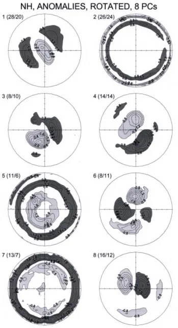
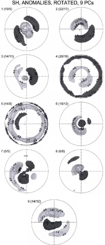
evo-Fig. 7. Scores of rotated PCs for NH. Each PC is indicated by its
number; the numbers of corresponding positive and negative types are given in parentheses. Contour interval is 0.4; zero and ±0.4 isolines are omitted; positive (negative) anomalies exceeding 0.8 (below −0.8) are in dark (light) shading.
lution. SH PC4 predominantly occurred in positive mode during the 1980s and negative mode in the 1990s. The in-verse behaviour holds for SH PC5. The latter PC score is fairly close to that of PC5 shown by Salles et al. (2001). In that study this spatial distribution appeared to be linked to the QBO. However, in this case there does not appear to be such a clear link. PC5- appears to occur most frequently in a westerly phase of the QBO, as well as PC4+, though during the first half of the sample only. In the second half, PC5+ and PC4- become more common but without any apparent relationship to the phase of the QBO.
In the NH summer PC2 appeared more frequently in a neg-ative mode in the 1980s and as a positive mode in the 1990s.
It should be noted that the PC2 difference between these decades is not as clear-cut as for the SH modes. NH PC5 was far more common during the 1980s, where it occurred mainly in positive and a few negative modes. After 1989 the few appearances were negative. NH PC7 became more com-mon in the late 1980s and 1990s, where it appeared mostly in positive mode. There is a hint of a possible decadal vari-ability in the occurrence of positive and negative types, but the sample is too short to be conclusive.
4.2.2 Winter type characteristics
The anomaly analysis shows enhanced variability for the SH winter when compared with the raw data analysis. It is in-teresting to note that features such as dipole or quasi-dipole anomalies (PC2, PC3, PC6, PC8) tend to resemble the ones obtained in the MSU Channel 4 temperature PC analysis (Salles et al., 2001). There are fairly frequent joint occur-rences of these PCs with their similar counterparts from the MSU analysis.
SH PC1, in positive mode, implies a PV weakening over the Antarctic and an enhancement over the South At-lantic/eastern South Pacific, as well as south of Australia. This can lead to an extended vortex along 45◦W–135◦E axis. The less frequent negative mode implies an enhance-ment over the Antarctic. The positive mode was detected throughout the sample, but has become more frequent during the last years of the sample. The negative mode is limited to the 1980s with a significant occurrence between 1986 and 1989. PC2 points to a meridional displacement of the polar vortex. In positive mode the vortex is displaced towards the western South Pacific, and in negative mode towards the In-dian Ocean. Both negative and positive modes are present throughout the sample. Nevertheless, the occurrence of one or the other mode seems to be modulated by a quasi-decadal oscillation. PC3 is the result of enhanced (weakened) vor-ticity over the eastern Indian Ocean and western South Pa-cific and an slight PV weakening (enhancement) over the Antarctica. The occurrence of this type shows that initially it was more common in positive mode and slowly the nega-tive mode became more frequent. The main change in phase took place between 1989 and 1991. This mode is absent in the last two years of the sample. PC6 shows the PV intensi-fication (weakening) in the vortex core and a weakened (in-creased) PV mainly over the South Atlantic. It is the first type to show a distinct oscillatory alternation between posi-tive and negaposi-tive modes, with an interval of about 14 years between sequences of similar sign. PC 7 is a more complex quadrupole structure, which is probably linked to the elon-gation of the vortex, while PC8 is similar to PC2 but much closer to the highest latitudes. PC7, with a rather limited number of events, appears in negative mode at the beginning of the sample and switches to positive mode towards the end. PC8 also shows an oscillatory phase behaviour with a peri-odicity similar to PC6. It became more frequent, in both pos-itive and negative modes during the 1990s. PC9 is similar to PC1 but perpendicular to it. This type also shows a change in
Fig. 8. Same as in Fig. 7 except for SH.
behaviour around 1990, having mostly positive modes during the 1980s and negative ones afterwards.
Though the present analysis better assesses the variability of the polar vortex, it is not easy to detect a distinct pattern of seasonal evolution from the PC set just described. Rather the above patterns, as would be expected, tend to show the predominance of wave 1 and to a lesser extent wave 2
quasi-stationary waves. It is interesting to observe that the PCs that describe the vortex in winter show positive PV anomalies, i.e. an enhancement of the vortex during 1987, and a weakening during 1988, in agreement with the ozone hole observations mentioned previously. The period between 1988 and 1991 seems to be a transition period in the evolution of the SH polar vortex. Many SH winter and summer modes show a change in polarity during that period, suggesting a change in the hemispheric circulation around that time.
The final breakup or warming of the SH hemisphere vortex appears to show more variability in its spatial structure in this analysis. This shows that the finer details in the final stages of the SH vortex can change from year to year, even though the general location of the process remains in the vicinity of the South Atlantic.
The NH vortex, which is not as symmetric, has anomaly PC winter types, which more closely resembles quasi-stationary wave 1 (PC3, PC4 and PC8) and 2 patterns (PC6), confirming that the NH vortex responds more to wave per-turbations than the SH one. Though present throughout the sample, PC1-, which describes an enhancement of the mean PV over the polar region and a weakening approximately over Europe and Alaska, was somewhat more frequent dur-ing the 1980s and PC1+ more frequent durdur-ing the 1990s. PC1+ seems to exhibit a quasi-decadal variability. PC3+, on the other hand was detected only during the 1980s. This im-plies a vortex displaced towards the North Pacific and Asia. The negative mode, though present throughout the sample, became more frequent in the 1990s, i.e. a vortex displaced towards Europe. PC4 is also a wave 1 pattern perpendicular to PC3. This type appears to respond very clearly to a quasi-decadal variability, both in positive and negative modes. This mode suggests an oscillation on the location of the vortex between North America and Central Asia. PC6 is the only wave 2 anomaly pattern, with a relatively reduced number of events. It seems to respond to a 4- to 5-year oscillation, which leads to the preferential occurrence of positive or neg-ative modes. It did not arise in the data set after 1993. The last winter mode, PC8, appears to represent a dipole between the Canada/Greenland and the North Pacific/Siberia. Both the positive and negative types are present throughout the sample. Nevertheless, there appears to be a 7-to 9-year pe-riod oscillation which favours the occurrence of one or the other of these.
4.2.3 NH sudden warming events
If we consider again the sudden warming issue, we find that warming events following Labitzke and Naujokat’s (2000) classification coincide mostly with PC1- and a couple coin-cide each with PC4- and PC8+. PC4- implies an enhance-ment of the PV field over Greenland and Northern Canada and a weakening over Russia, while PC8+ implies a weaken-ing over Greenland and Eastern Canada and a strengthenweaken-ing over Siberia.
Inspection of the NH PC types during the last two months of each vortex life cycle, as determined by the raw data
analysis, show more homogenous results than over the SH. Though interannual variability remains significant, a few PCs dominate, in particular PC1+, PC1-, PC3-, PC4+ and PC4-. 4.3 Comparison of raw data vs. anomalies analysis and
dis-cussion
Results based on raw data and anomalies have been pre-sented. There may be some initial confusion, since the two analyses may not appear to agree with each other. However, in this subsection it is argued that they must be looked upon as complementary rather than competing.
First, we give the answer to why several summer types are revealed in anomalies, while a single summer type is iden-tified in the raw data. As mentioned in the methodology, the analysis of raw data is sensitive mainly to a strong fea-ture, such as the intensity and position of the polar vortex, whereas the analysis of anomalies reflects the position of PV anomalies, but not their intensity. In summer, PV fields are only weakly disturbed, and the differences between individ-ual monthly patterns are too subtle to be detected in the raw data analysis. On the other hand, for the anomaly analysis, the amplitude of disturbances is not relevant, and even very weak anomalies, if they consistently and repeatedly occur, may lead to a definition of a separate type.
The two analyses divide a year into winter and summer parts in different ways. According to the raw data analysis, summer is the period without a polar vortex feature. In the anomaly analysis, summer can be defined as the period oc-cupied mostly by types with weak, annular-like anomalies in lower latitudes, i.e. when there is no significant planetary wave activity. The raw-data-based and anomaly-based sum-mers do not coincide: the former tends to last longer. The reason is in the transition months (April, September and Oc-tober in NH, March, April and December in SH) which ap-pear as summer types for the raw data but as winter types in the anomaly study. Wave activity, though weak when com-pared to the winter period, is still present during these months and is picked up by the latter analysis.
Since the anomaly analysis is able to pick the finer de-tails in the year-to-year changes, the SH winter anomalies also shows more variability than the raw data analysis. The inspection of NH raw data show larger intraseasonal vari-ability in winter, which is similarly reflected in the anomaly fields. The discrepancy between the anomaly and raw types in the SH and the better correlation between both sets in the NH could be due to the fact that in the NH the shorter-lived, weaker polar vortex responds better to the stronger wave ac-tivity there. Such consistency, or inconsistency (in the SH), between raw and anomaly analysis is useful in assessing the contribution of driving mechanisms to the observed variabil-ity.
An interesting result from both the raw and the anomaly analysis shows that there seems to have been a change in the distribution of the PV field between the 1980s and the 1990s. This change was prominent in a larger number of modes over the SH. Two of the modes could even exhibit what appears
to be a quasi-decadal variability. Though also present in the NH, more prominent temporal variabilities with periods between 5 and 10 years seem to coexist there. This result seems to be consistent with the fact that NH sudden warming events became far less frequent during the second half of the sample. It should be noted that, as shown in Labitzke and Naujokat (2000), the latter years of the sample and the win-ters through 2000 show considerable variability, a probable warming trend in the February 10 hPa temperature and minor warming events.
It may appear that the Mt. Pinatubo eruption could have been responsible for the apparent multi-annual cycles. How-ever this is not the case. In first place, El Chich´on did not similarly affect the long-term trends. Secondly, the volcanic aerosol effect detected in the MSU lower stratospheric tem-peratures was basically limited to the tropics and lower sub-tropics, at least in the SH, and only lasted for approximately two years after the eruptions (Compagnucci et al., 2001). Note that, as mentioned above, the changes in PV started sometime around 1988–1989, two years before this last ma-jor eruption.
It is interesting to note that changes in the evolution of the ozone depletion have also been observed around that time, particularly over the SH (WMO, 1998). The mid-latitude SH ozone trends discussed in Malanca et al. (manuscript in preparation, 2002) show as well that these changes are lon-gitude, as well as seasonal dependent. Salles et al. (2001) also noted a change in the occurrence of some of the PC’s corresponding to the MSU lower stratosphere temperature anomaly. The tropopause height analysis by Steinbrecht et al. (1998, their Figs. 7 and 8) also shows a change in the trend around the same time. The Hohenpeissenberg ra-diosonde temperature retrievals at 5 Km and the tropopause height show a simultaneous decrease in the warming trend and height increase, respectively, around 1990. Their plots also show a weaker trend prior to the late 70s. Thus, this change would not be limited to the stratosphere. 100 hPa Antarctic radiosonde temperatures (Randel and Wu, 1999) show for a number of stations a stepwise behaviour, with fairly stable temperatures prior to the mid 1970s, followed by a decrease during the 1980s, and a new stable or weaker neg-ative trend arising between 1985 and 1990, approximately. Such an evolution is longitude and seasonal dependent. Their MSU Arctic analysis does not show such a distinct stepwise behaviour, thus also agreeing with the present results, i.e. fewer modes in the NH show the stepwise evolution around 1990. Thus, the change around 1990 can be consistently ob-served in a number of independent stratospheric data sets and variables, such as NCEP-derived PV, TOMS total ozone, ra-diosonde and MSU temperatures. Furthermore, these were studied using different statistical approaches. Hence, it ap-pears that it is a significant component in the temporal evo-lution of the lower stratosphere, at least over the SH. Some of the time series used in the other analyses mentioned begin in the early 1960s and show a fairly stable behaviour prior to mid 1970s. This could suggest a possible change to, or a trend towards, a new equilibrium state.
5 Conclusions
We presented an analysis that attempted to find typical (re-current) patterns in the monthly mean PV field at the 650 K isentropic level. For such an analysis, principal component analysis in T-mode, which is suitable for classification, was used. It was shown that different numbers of PCs, and both raw data and anomalies, yield meaningful and interpretable types. The rotated PCs should be given preference to the unrotated ones in such a type of analysis, after adequate in-spection and comparison between the observed fields (either raw or anomaly) and the corresponding PCs. A simultane-ous examination of classifications based on different num-bers of PCs and different kinds of input data (raw vs. anoma-lies) appears to be advantageous, as different classifications may uncover different complementary features and charac-teristics. The combined use of raw and anomaly analysises can be used to determine the nature of the variability.
The analysis successfully revealed well-known important features of stratospheric circulation, such as major mid-winter warmings in the NH, their absence in SH, early or late breakdowns of the polar vortex, and volcanic signatures. It was not possible with the current time series to identify possible ENSO features, particularly in the SH.
The present study has revealed, in agreement with other observations, a change in behaviour of the hemispheric PV fields during the years around 1990. Such a change appears to be an important feature of climate evolution during the last 25 years, given that it may be observed in various data sets. However, it is not yet possible to explain what processes have led to this change. The main point is that the present study was able to summarise previous independent findings regarding various aspects of polar vortex dynamics within the framework of a single analysis, which set out to determine a stratospheric PV climatology. It is clear that, while specific events, such as NH stratospheric warmings, are easily deter-mined using the present methodology, the development of a dynamic climatology will require a longer time series.
In further studies aiming in this direction, the analysis do-main should be extended to other levels and other variables, in order to cover the manifestations of the stratospheric cli-mate in all its complexity. Also, longer time periods should be investigated, so that the effects of phenomena with longer or variable periodicity (e.g. ENSO, solar cycle), as well as longer term trends, could be identified. While this is cer-tainly possible for the NH, current reanalysis products ex-tending time series back to the 1960s or even 1950s should be viewed with care, due to the scarcity of ground-based ob-servations in the SH. The introduction of satellite retrievals, starting in 1979, has a larger impact on reanalysis products over the SH.
We have thus shown the applicability of the T-mode PCA classification, to understand features of the stratospheric cir-culation, as well as a possible evolution. In our opinion it has the potential to uncover little understood features and vari-ability mechanisms. We believe we managed to prove that joining the physical knowledge with statistical know-how
could benefit stratospheric research, providing new insights in the field of stratospheric dynamics and climatology. Acknowledgements. The authors wish to thank the NCEP for
mak-ing available the reanalysis products used in the present study. The study was supported by the Grant Agency of the Academy of Sci-ences of the Czech Republic, project B3042004, Inter American In-stitute for Climate Change Studies Grant IAI-ISP-3-076 and the Ar-gentine Agencia Nacional par la Promoci´on de la Ciencia y la Tec-nolog´ıa grant PICT 97-02197 and PICT 99-06588. R.H. is grateful for the SPARC financial support for his attendance to the SPARC 2000 General Assembly, from which the paper has much benefited. This paper is a contribution to the European Comission EuroSPICE Project.
Topical Editor D. Murtagh thanks a referee for his help in eval-uating this paper.
References
Baldwin, M. P. and Dunkerton, T. J.: The stratospheric major warm-ing of early December 1987, J. Atmos. Sci., 46, 2863–2884, 1989.
Barnston, A. G. and Livezey, R. E.: Classification, seasonality and persistence of low-frequency atmospheric circulation patterns, Mon. Wea. Rev., 115, 1083–1126, 1987.
Bretherton, C. S., Smith, C., and Wallace, J. M.: An intercompar-ison of methods for finding coupled patterns in climate data, J. Climate, 5, 541–560, 1992.
Chen, P., Holton, J. R., O’Neill, A., and Swinbank, R.: Quasi-horizontal transport and mixing in the Antarctic stratosphere, J. Geophys. Res., 99, 16 851–16 866, 1994.
Cheng, X. and Dunkerton, T. J.: Orthogonal rotation of spatial pat-terns derived from singular value decomposition analysis, J. Cli-mate, 8, 2631–2643, 1995.
Compagnucci, R. H. and Ruiz, N. E.: On the interpretation of prin-cipal component analysis as applied to meteorological data, Proc. 5th Int. Meeting on Statist. Climatol., Toronto, 241–244, 1992. Compagnucci, R. H. and Salles, M. A.: Surface pressure patterns
during the year over southern South America, Int. J. Climatol., 17, 635–653, 1997.
Compagnucci, R. H. and Vargas, W. M.: Patterns of surface pres-sure field during July 1972–1983 in southern South America and the Antarctic peninsula, 3rd Int. Conference on Statistical Clima-tology, Vienna, 1986.
Compagnucci, R. H., Salles, M. A., and Canziani, P. O.: The spatial and temporal behaviour of the lower stratospheric temperature over the Southern Hemisphere: The Msu view, Part II, spatial behaviour, Int. J. Climatol., 21, 439–454, 2001.
Drosdowsky, W.: An analysis of Australian seasonal rainfall anomalies: 1950–1987. I: Spatial analysis, Int. J. Climatol., 13, 1–30, 1993.
Eder, B. K., LeDuc, S. K., and Sickles II, J. E.: A climatology of total ozone mapping spectrometer data using rotated principal component analysis, J. Geophys. Res., 104, 3691–3709, 1999. Erlebach, P., Langematz, U., and Pawson, S.: Simulations of
strato-spheric sudden warmings in the Berlin troposphere-stratosphere-mesosphere GCM, Ann. Geophysicae, 14, 443–463, 1996. Fairlie, T. D. A. and O’Neill, A.: The stratospheric major warming
of winter 1984/85: observations and dynamical inferences, Q. J. Roy. Meteorol. Soc., 114, 557–578, 1988.
Huth, R.: An example of using obliquely rotated principal compo-nents to detect circulation types over Europe, Meteorol. Z., N. F., 2, 285–293, 1993.
Huth, R.: PCA-based classification of circulation and weather pat-terns: Some methodological considerations, Proc. 6th Int. Meet-ing on Statist. Climatol., Galway, Ireland, 155–158, 1995. Huth, R.: An intercomparison of computer-assisted circulation
clas-sification methods, Int. J. Climatol., 16, 893–922, 1996a. Huth, R.: Properties of the circulation classification scheme based
on the rotated principal component analysis, Meteorol. Atmos. Phys., 59, 217–233, 1996b.
Huth, R.: Continental-scale circulation in the UKHI GCM, J. Cli-mate, 10, 1545–1561, 1997.
Kalnay, E., Kanamitsu, H., Kistler, R., et al.: The NCEP/NCAR 40-year reanalysis project, Bull. Amer. Meteorol. Soc., 77, 437–471, 1996.
Kodera, K.: Influence of volcanic eruptions of the troposhpere through stratospheric dynamical processes in the Northern Hemi-sphere winter, J. Geophys. Res., 99, 1273–1282, 1994.
Labitzke, K. G. and van Loon, H.: The Stratosphere: Phenomena, History, and Relevance, Springer, 179 pp., 1999.
Labitzke, K. G. and Naujokat, B.: The lower Arctic stratosphere in winter since 1952, SPARC Newsletter, 15, 11–14, 2000. Michelangeli, P. A., Vautard, R., and Legras, B.: Weather regimes:
Recurrence and quasi stationarity, J. Atmos. Sci., 52, 1237–1256, 1995.
North, G. R., Bell, T. C., Cahalan, R. F., and Moeng, F. J.: Sampling errors in the estimation of empirical orthogonal functions, Mon. Wea. Rev., 110, 699–706, 1982.
O’Lenic, E. A. and Livezey, R. E.: Practical considerations in the use of rotated principal component analysis (RPCA) in diagnos-tic studies of upper-air height fields, Mon. Wea. Rev., 116, 1682– 1689, 1988.
Perlwitz, J. and Graf, H.-F.: The statistical connection between
tropospheric and stratospheric circulation of the northern hemi-sphere winter, J. Climate, 8, 2281–2295, 1995.
Pierce, R. B. and Fairlie, T. D. A.: Observational evidence of pre-ferred flow regimes in the Northern Hemisphere winter strato-sphere, J. Atmos. Sci., 50, 1936–1949, 1993.
Randel, W. and Wu, F.: Cooling of the Arctic and Antarctic Polar stratospheres due to ozone depletion, J. Climate, 12, 1476–1479, 1999.
Richman, M. B.: Rotation of principal components, J. Climatol., 6, 293–335, 1986.
Richman, M. B., Angel, J. R., and Gong, X.: Determination of di-mensionality in eigenanalysis, Proc. 5th Meeting on Statist. Cli-matol., Toronto, 229–235, 1992.
Salles, M. A., Canziani, P. O., and Compagnucci, R. H.: The spatial and temporal behaviour of the lower stratospheric temperature over the Southern Hemisphere: The Msu view, Part I, Method-ology and temporal behaviour, Int. J. ClimatMethod-ology, 21, 419–437, 2001.
Serrano, A., Garc´ıa, J. A., Mateos, V. L., Cancillo, M. L., and Gar-rido, J.: Monthly modes of variation of precipitation over the Iberian Peninsula, J. Climate, 12, 2894–2919, 1999.
Steinbrecht, W., Claude, H., K¨ohler, U., and Hoinka, K. P.: Correla-tion between tropopause height and total ozone: implicaCorrela-tions for long-term ozone trends, J. Geophys. Res., 103, 19 183–19 192, 1998.
Toth, Z.: Preferred and unpreferred circulation types in the northern hemisphere wintertime phase space, J. Atmos. Sci., 50, 2868– 2888, 1993.
Waugh, D. W. and Randel, W. J.: Climatology of Arctic and Antarc-tic polar vorAntarc-tices using ellipAntarc-tical diagnosAntarc-tics, J. Atmos. Sci., 56, 1594–1613, 1999.
WMO: Scientific assessment of ozone depletion 1998, Global Ozone Research and Monitoring Project report no. 44, World Meteorological Organization, 1998.